CIRTEN
Consorzio Interuniversitario per la Ricerca TEcnologica Nucleare
Lavoro svolto in esecuzione dell’Attività LP2. C1
AdP MSE-ENEA sulla Ricerca di Sistema Elettrico - Piano Annuale di Realizzazione 2013
UNIVERSITÀ
POLITECNICO DI TORINO
Development of the neutronic module and
benchmark and validation of the thermal-hydraulic module
of the FRENETIC code
Autori
Roberto Bonifetto, Dominic Caron, Sandra Dulla, Laura Savoldi Richard, Piero Ravetto, Roberto Zanino (PoliTo)
Alessandro Del Nevo (ENEA)
CERSE-POLITO RL 1500/2014
Index
Abstract _______________________________________________________ 2
1
Introduction ________________________________________________ 3
2
Benchmark and validation of the thermal-hydraulic module _________ 4
2.1
Computational domain and boundary conditions_______________ 4
2.1.1 Boundary Conditions ________________________________________________ 6
2.2
Comparison between FRENETIC and RELAP5-3D© TH models _ 6
2.3
Results and discussion _____________________________________ 8
2.3.1 Benchmark of FRENETIC Against RELAP5-3D© ________________________ 8 2.3.2 Validation of FRENETIC against EBR-II experimental data ________________ 11
2.4
Conclusions and perspective _______________________________ 15
3
Development of the neutronic module __________________________ 15
3.1
Introduction ____________________________________________ 15
3.2
Adjoint capabilities of the neutronic module __________________ 16
3.3
Quasi-static capabilities of the neutronic module ______________ 17
3.4
Representative results ____________________________________ 19
3.4.1 Compensated transient _____________________________________________ 19 3.4.2 Divergent transient with non-linear feedback ____________________________ 21
3.5
Conclusions ____________________________________________ 22
4
References _________________________________________________ 22
Abstract
The simulation of the dynamic behavior of Lead-cooled Fast Reactors (LFR) is a key step in the development of this innovative nuclear technology. To this aim, computational tools for the coupled neutronic/thermal-hydraulic description of the reactor core need to be developed. This task can be carried out at different levels of complication. Some codes are characterized by a highly detailed description of the system components, but they also require a high computational cost.
At Politecnico di Torino the research group of nuclear engineering has been developing the FRENETIC code for the dynamic simulation of LFR cores with closed hexagonal fuel elements at a reduced computational cost, suitable for parametric evaluations and simulations of safety-related transients. The code separately solves the neutronic and thermal-hydraulic model equations, with neutronic/thermal-hydraulic feedback introduced through a coupling procedure. The work carried out during this year activity has been focused on two main topics
1) validation of the thermal-hydraulic module performing various benchmark exercises (activity performed in collaboration between POLITO and ENEA)
2) extension of the capabilities of the neutronic module to include the quasi-static method demonstrating the new functionality of the code with example scenarios, one of which includes thermal-hydraulic feedback.
1
Introduction
Several activities are ongoing in Europe and in particular in Italy around the development of the GenIV lead-cooled fast reactor (LFR) [1]. The main concepts which evolved over the years are those of the ELFR (the first-of-a-kind EU reactor) [2], of ALFRED (the EU demonstrator) [3] and of MYRRHA (the EU technology pilot plant) [4]. Indeed, Ansaldo Nuclear, ENEA and the Institute of Nuclear Research of Romania have signed at the end of December 2013 an agreement for the establishment of the Falcon Consortium (Fostering Alfred Construction), whose objective is to construct ALFRED in Romania.
Within that framework, the FRENETIC (Fast REactor NEutronics/Thermal-hydraulICs) code has been recently developed for the simulation of coupled neutronic/thermal-hydraulic transients in LFR with the core arranged in hexagonal assemblies (briefly HAs in the following), enclosed in a duct [5]. The code has the ambition to provide fast approximate solutions for core design and/or safety analysis, and this thanks to the fact that the 3D problem is solved with a simplified approach. The neutronic (NE) module in FRENETIC includes the options of point kinetics [6] and of a full 3D time dependent multigroup diffusion solver [7]. The thermal hydraulic (TH) module of FRENETIC solves the 1D (axial) mass momentum and energy conservations laws of the coolant, together with the 1D (axial) heat conduction equation in the fuel pins, in each assembly. The assemblies are then thermally coupled to each other on each horizontal cross section of the core, leading to a quasi-3D model, as it will be detailed below.
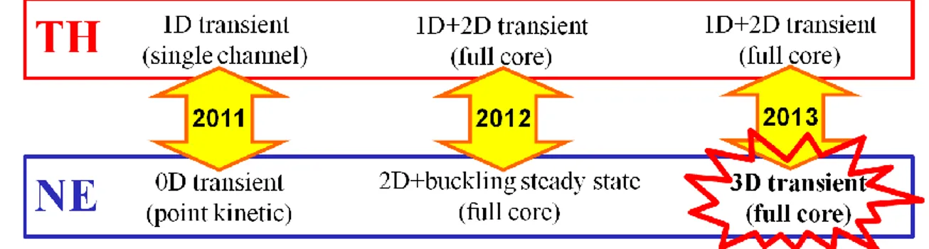
The work carried out in 2014 continues the development of this computational tool, following the previous steps carried out starting from year 2011 and summarized in Fig. 1, while Fig. 2 sketches the coupling strategy that has been adopted from the beginning of the project, allowing the possibility to perform separately the development and validation of the NE and TH modules.
Fig. 1. Evolution of the modelling capabilities of the FRENETIC code.
The research activity of the present year has been focused on two specific topics:
1) the validation of the thermal-hydraulic module, performing various benchmark exercises against other computational tools such as RELAP and participating to the benchmark activity on the EBR-II reactor (activity performed in collaboration between POLITO and ENEA); this part has been presented at the International Topical Meeting on Advances in Thermal Hydraulics, Embedded Topical Meeting of the 2014 ANS Annual Meeting in Reno, NV (USA), on June 15-19, 2014, and published in the transactions of that conference [8].
2) the extension of the capabilities of the neutronic module to include the quasi-static method; the adjoint flux calculation has been implemented into the NE module, allowing the correct determination of the kinetic parameters, and different quasi-static approaches have been coded to compare their performances.
2
Benchmark and validation of the thermal-hydraulic
module
The TH module of FRENETIC was already validated in the case of a single assembly against data from the Lead-Bismuth Eutectic (LBE) CIRCE integral experiment at ENEA Brasimone [9]. In order to validate the multi-assembly TH capabilities of FRENETIC and in the absence of easily available data for lead-cooled multi-assembly structures, we consider as an alternative reference the experimental data of the sodium-cooled EBR-II reactor [10], which was operated between 1965 and 1995 at Argonne National Lab (USA). This choice provides a twofold advantage: 1) the availability of simulations performed within the framework of a multi-party benchmarking exercise coordinated by the IAEA [11] and in particular the results obtained with the RELAP5-3D© code [12] during the blind phase of the benchmark; 2) the existence of some experimental data, made available by IAEA to the benchmark participants, after the blind phase.
The work is organized as follows: first we identify the computational domain and define the boundary conditions for the different tests (steady-state and transient) that we are going to analyse. Then, we give a brief comparative description of the TH models as implemented in FRENETIC and in RELAP5-3D©, as well as of the part of the experimental set-up which is relevant for this exercise. Finally, the results of the FRENETIC and RELAP5-3D© simulations are presented and discussed, in comparison to each other, and the FRENETIC results are compared to the experimental data.
2.1 Computational domain and boundary conditions
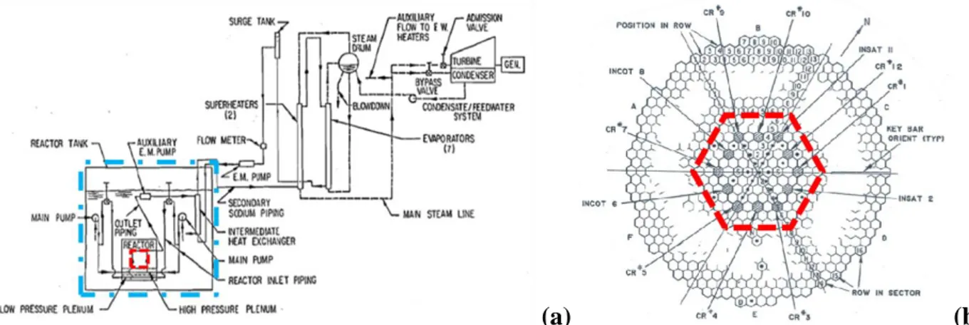
A sketch of the EBR-II cooling circuit is shown in Fig. 3a. While the RELAP5-3D© model extends to the primary cooling system, with two 3D components representing the reactor zone and the pool region (containing the high and low pressure flow lines, the heat exchangers and the so-called Z-pipe modeled as 1D components), the FRENETIC computational domain is limited in the axial direction to the bundle region of the core (0.61 m axial extension in the EBR-II case) and in the radial direction to the central 7 rings (R1 to R7) of the core, including 127 HAs, i.e. to the region inside the red dashed hexagon in Fig. 3b, connected with the high pressure inlet plenum. Each HA of the 7 innermost rings is modeled by a 1D component in RELAP5-3D©. The outer rings corresponding to the blanket or the reflector HAs are modeled with 24 equivalent
1D pipes: two pipes (one for the blanket and one for the reflector HAs) for each of the 12 sectors used for the azimuthal discretization.
(a) (b)
Fig. 3 (a) Sketch of the EBR-II cooling circuit and boundary of the computational domain for the FRENETIC model (dashed red line) and for the RELAP5-3D© model (dash-dotted cyan line). (b) Reactor core cross
section and radial boundary of the computational domain for the FRENETIC model (dashed red line).
The EBR-II core loading pattern is rather complicated and shown in Fig. 4. The fuel alloy uniquely developed and fabricated for the EBR-II reactor is called U-5FS [11]. The composition of all HAs is faithfully reproduced by both FRENETIC and RELAP5-3D©, with the only exception of the partial driver (fuel) HAs, which are half stainless steel (SS) and half U-5FS, but modelled as all U-5FS in FRENETIC. This is due to a limitation of the model currently implemented in FRENETIC: at present, for each HA, we can compute at each height (z) only a single solid temperature, so that it is impossible for us to rigorously distinguish between fuel and SS pins. However, in order to take into account, at least approximately, this important difference, the actual number of fuel pins is conservatively considered, applying the heat source only to them, whereas the SS pins are taken into account only for the computation of the flow area and of the hydraulic diameter (neglecting their heat capacity).
(a) (b)
Fig. 4 (a) EBR-II core loading pattern. (b) Composition of the main HA types (BES, LUM 2 and XY-16 are SS HAs geometrically similar to the R, XX10 and XX09 HAs, respectively).
Besides the composition, also the structure of the different HAs has been carefully modelled. We can distinguish among three main groups:
1) the fuel HAs ("D" in Fig. 4), the “experimental” HAs ("X###" in Fig. 4) and the “K” HA s, made of an hexagonal wrapper and containing different number of pins of different mat erials;
2) the reflector HAs ("R" in Fig. 4), made of an hexagonal wrapper and containing an hexag onal SS block;
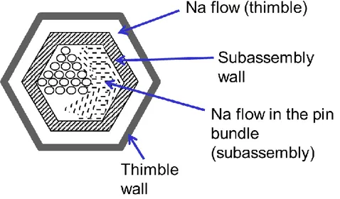
3) the control rod HAs ("C" in Fig. 4), the safety rod HAs ("S" in Fig. 4) and the “instrumen ted” HAs ("XX09" and "XX10" in Fig. 4), which are made according to the so-called box -in-the-box concept, as shown in Fig. 5.
While the model of the HAs in the former two groups is similar in FRENETIC and RELAP5-3D©, there are non-negligible differences in the model of the HAs in the third group, as it will be discussed below.
Fig. 5 Box-in-the-box HA type as adopted for control rod HAs, safety rod HAs and “instrumented” HAs.
2.1.1 Boundary Conditions
RELAP5-3D© is used to provide FRENETIC with detailed boundary conditions (BC) at the inlet and outlet of each HA in both steady state and transient analyses. In the axial direction FRENETIC uses as BC the distribution of the inlet mass flow rate, see Fig. 6a, and of the outlet pressure pout = 2.2-3.1 bar among the different HAs, computed by RELAP5-3D©, as well as the almost uniform inlet temperature Tin= 625 K. In the radial direction, an adiabatic BC is assumed by FRENETIC between R7 and the rest of the core, i.e. the blanket region. Moreover, the input power distribution among HAs is provided by Argonne, see Fig. 6b, and assumed here to be axially uniform over the active 0.31 m.
2.2
Comparison between FRENETIC and RELAP5-3D© TH models
As far as the coolant is concerned, both FRENETIC and RELAP5-3D© solve 1D transient mass, axial momentum and energy balances for the evolution of the sodium temperature profile TNaj (z,
As far as the solid (U-5FS, SS, other) pins are concerned, 1D axial transient heat conduction is solved in FRENETIC (neglecting both the cladding and the gap, and assuming adiabatic endings) for <Tfuel(z, t)>, coupled with the Na, where the average < > is computed on the entire solid cross section at a given core height z in each HA, while a steady state parabolic profile is assumed for Tfuel(r). On the contrary, 1D radial transient heat conduction is solved in RELAP5-3D© (including both the cladding and the gap in the model), neglecting axial heat conduction in the pins. The nature of the FRENETIC model of the pins is more a heritage of its origins in the context of nuclear fusion applications [13] than an actual need in a fission application like the present one. Indeed, the inclusion of radial heat conduction in the FRENETIC model is envisaged in a future version of the code.
(a) (b)
Fig. 6 (a) Distribution among HAs of the inlet mass flow rate (kg/s) computed by RELAP5-3D© and used as BC by FRENETIC. (b) Distribution among HAs of the input power (MW).
Considering the fact that the main purpose of this work is to provide the first benchmark and validation of the TH module of FRENETIC in a multi-HA situation, the nature of the thermal coupling model between neighboring HAs plays a quite fundamental role. In FRENETIC HAs j and k sharing a side of the hexagon exchange heat through a heat transfer coefficient which results from the series of: convective resistance in HAj / conduction through the wrapping j / conduction through the Na, assumed stagnant, in the gap between neighboring HAs / conduction through the wrapping k / convective resistance in HAk. (Concerning the stagnation assumption, this is justified by the fact that, according to the RELAP5-3D© simulation, the fraction of the total mass flow rate flowing in the gap is ~ 0.2 %, resulting in an initial coolant speed in the inter-HA gap < 0.1 m/s, i.e., much smaller than the initial speed in the HAs, which is typically > 1 m/s.) On the contrary, in RELAP5-3D© the bypass is modeled as part of the reactor 3D component (5 radial zones, 12 azimuthal sectors and 17 axial nodes), where each node is thermally coupled with the HAs at the corresponding location and the coupling between neighboring HAs j and k involves the series of convective resistance in HAj / conduction through the wrapping j / convective resistance in the gap towards HAj / convective resistance in the gap towards HAk / conduction through the wrapping k / convective resistance in HAk, while the heat conduction in the Na is not modeled by RELAP5-3D©. At steady state, the resulting thermal resistance between neighboring HAs in RELAP5-3D© is about 1.25 times that in FRENETIC.
As mentioned above, the main discrepancy in the model of a single HA appears in the case of the box-in-the-box type, see Fig. 5. In FRENETIC the Na in the outer channel (thimble) is assumed stagnant (the total mass flow rate being imposed in the subassembly) and the additional thermal
conduction resistance to the inter-HA (xy) coupling is accounted for through the series of Na in the thimble and SS of the sub-assembly wall. On the contrary, in RELAP5-3D© also the Na flow in the thimble region is accounted for, so the cooling of the assembly is partially taken care of by the coolant in that region.
As a final comment, it should be noted that, in the FRENETIC model, both the Na where it is assumed stagnant (i.e., in the gap between neighboring HAs and in the thimble region in the box-in-the-box HAs) and the HA SS hexagonal wrapping contribute only to the thermal resistance, whereas their thermal capacity is neglected. The thimble Na heat capacity should account for ~ 45 % of the total Na heat capacity in the box-in-the-box, whereas the wrapping heat capacity should account for ~ 1-30 % of the total solid heat capacity of the HA, depending on the HA type.
2.3 Results and discussion
This section is divided in two parts: in the first one, the benchmark of FRENETIC against RELAP5-3D© is presented; in the second one, the validation of FRENETIC is presented against a set of experimental data from the EBR-II.
We first consider steady state operation under two different assumptions: a) adiabatic HAs -- a non-realistic condition, considered here for the only sake of benchmarking FRENETIC against RELAP5-3D© first in a simplistic situation; b) thermally coupled HAs. One transient is then simulated starting from the steady state experimental data of the Shutdown Heat Removal Test SHRT-17, and namely c) the loss-of-flow due to the trip of the primary and intermediate pumps of EBR-II, suddenly followed by a SCRAM (protected loss-of-flow).
2.3.1 Benchmark of FRENETIC Against RELAP5-3D©
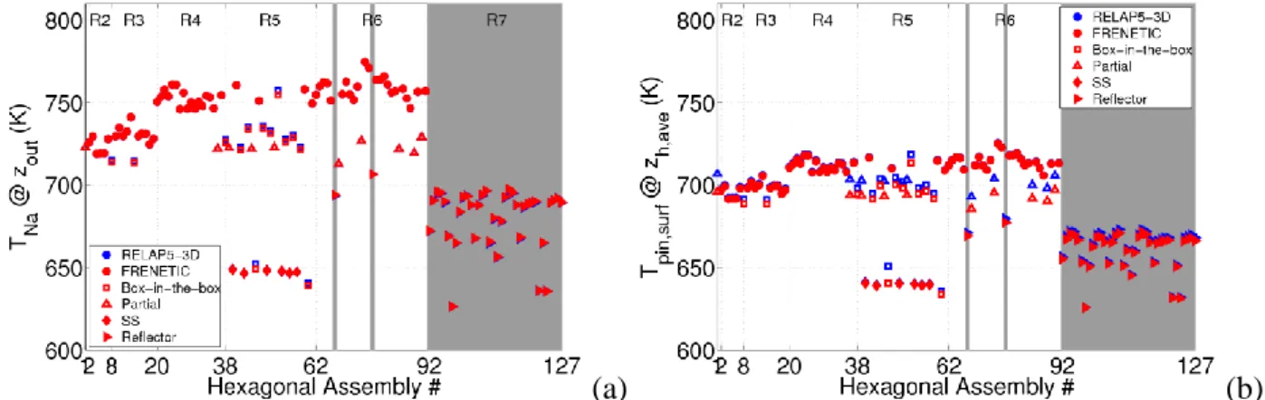
The first comparison refers to the steady-state case when the HAs are fictitiously assumed to be adiabatic. In this case, a very good agreement is expected, as the accuracy of, e.g., the outlet Na temperature Tout depends only on the conservation of energy in each HA. Indeed, it is seen in Fig. 7a that the agreement between the two is very good. The only non-overlapping symbols correspond to the slightly lower Tout computed in the inner channel of the box-in-the-box HAs by FRENETIC, related to the fact that in the FRENETIC model the whole HA mass flow rate (the sum of the subassembly one and the thimble one, see Fig. 5) flows in the subassembly (as the Na is assumed stagnant in the thimble), so that for a given input power the enthalpy increase of the sodium in the central part of the HA is lower than predicted by RELAP5-3D©, where the flow is split between subassembly and thimble. The pin surface temperature distribution computed in the different HAs is shown in Fig. 7b. Besides the box-in-the-box HAs, discrepancies arise also in the partial fuel HAs: indeed, the simplifying assumption of all U-5FS pins made in FRENETIC means that the same input power is spread over twice as many pins as in RELAP5-3D©, which obviously leads to lower pin surface temperature. However, for the rest of the HAs the steady state parabolic profile model works quite well. A detailed comparison of the radial profiles inside the pins (not shown here) indicates that the agreement in the pin central temperature is also good, except however in the most important case of the fuel pins: here FRENETIC underestimates (by 30-40 K) the RELAP5-3D© values, most likely as a consequence of having
neglected the gap and the cladding: the lower thermal conductivity of the latter (~ 22 W/m K) compared to that of U-5FS ( ~ 30 W/m K) gives rise to a steeper temperature profile in the cladding, resulting in a higher central temperature.
(a) (b)
Fig. 7 Comparison between FRENETIC (red symbols) and RELAP5-3D© (blue symbols) at steady state, assuming adiabatic HAs: (a) Tout; (b) average pin surface temperature at mid height of the heated region.
Solid circles refer to all driver and experimental HAs.
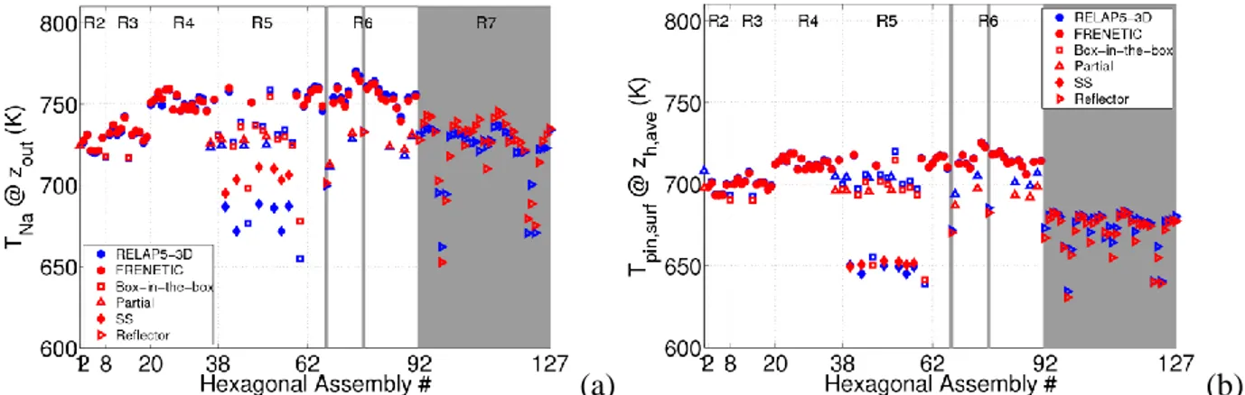
The second comparison refers to the steady-state case when the HAs are thermally coupled to their neighbors, as discussed above. The results of the comparison are shown in Fig. 8 and 9. In Fig. 8, we see the homogenizing effect of the thermal coupling between neighboring HAs, especially noticeable in the case of the coldest HAs; this effect is weaker in RELAP5-3D© than in FRENETIC, because of the above-mentioned higher thermal resistance between adjacent HAs. The quantitative comparison between outlet Na temperatures and also pin surface temperatures at mid height of the heated region is shown in Fig. 9. It is seen in Fig. 9a that there is good agreement in all driver HAs, while the stronger thermal coupling in FRENETIC gives rise to an overestimation of Tout in the colder ones, e.g. the SS HAs. The adiabatic BC on the outer side of R7 in FRENETIC causes a general overestimation of the temperature in the reflector HAs. As to the pin surface temperature distribution across the mid height core cross section, see Fig. 9b, it is seen that there is good agreement in all HAs where the same model is adopted by the two codes, whereas the temperature is overestimated by FRENETIC in the colder HAs and especially in SS HAs because of the stronger coupling combined with the relatively low temperature and relatively low mass flow rate, see Fig. 6a.
(a) (b) (c)
Fig. 8 Computed Na temperature (K) distribution at the outlet of the heated region: (a) FRENETIC, adiabatic HAs; (b) FRENETIC, coupled HAs; (c) RELAP5-3D©, coupled HAs.
(a) (b)
Fig. 9 Comparison between FRENETIC (red symbols) and RELAP5-3D© (blue symbols) at steady state, in the case of thermally coupled HAs: (a) Tout; (b) average pin surface temperature at mid height of the heated
region. Solid circles refer to all driver and experimental HAs.
The third comparison refers to the transient case defined above, i.e. a protected loss-of-flow. The evolution of the input power and of the total mass flow rate in the part of core considered for the present exercise, i.e. the inner core (R1 to R5) and the extended core (R6 and R7), is shown in Fig. 10. As explained above, this evolution of the mass flow rate is computed by RELAP5-3D© and used by FRENETIC as inlet boundary condition. The SCRAM is triggered at the start of the loss of flow and is modeled scaling down the power input in each HA according to the global power evolution. No neutronics is included in the model, for the time being, although this is planned for the next step, thanks to the coupled neutronics/thermal-hydraulics model implemented in FRENETIC.
Fig. 10 Evolution of the driver of the transient considered in the present work: normalized Na mass flow rate computed by RELAP5-3D© and used by FRENETIC as boundary condition (left axis); normalized input
power [11] (right axis).
The evolution of the temperature can already be qualitatively predicted by considering Fig. 10: in the initial phase the power decreases faster than the mass flow rate and the temperature will therefore decrease, but then the mass flow rate decreases faster than the power and the temperature will increase again, before finally decreasing due to the combined increase of the mass flow rate (natural circulation) and the power going asymptotically to zero.
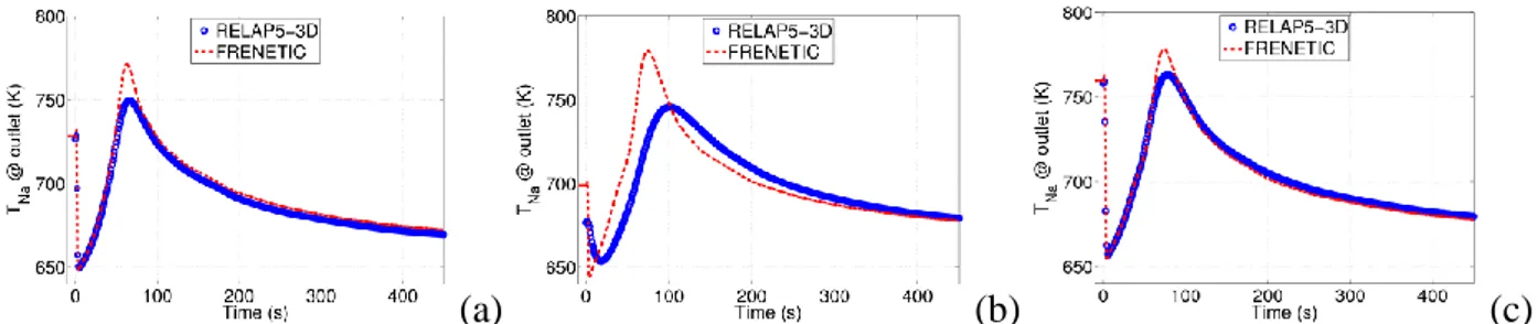
The computed evolution of the Na temperature at the outlet of three selected HAs is reported in Fig. 11 and qualitatively reproduces the expectations. The transient is characterized by three phases: initially the temperature drops stepwise, mainly as a consequence of the rector SCRAM. Then the temperature increases again, due to the reduction of the mass flow rate; finally the temperature drops again as the mass flow rate increases again due the natural circulation induced by the temperature increase due in turn to the residual input power (decay heat). The agreement between FRENETIC and RELAP5-3D© is very good in the driver HA and in the experimental HA, except for an overestimation of the peak, which is due to the fact that the thermal capacity of the SS wrapper and of the Na in the gap between neighbouring HAs are not taken into account in the FRENETIC model. On the contrary, in the XX10 HA the agreement is only qualitative, which can be explained by observing that for that HA (of the box-in-the-box type) also the thermal capacity of the Na in the thimble and of the SS subassembly wall are neglected, thus inducing a non-negligible difference between the results of the two models. Moreover, for this HA the Na mass flow is almost equally split in the subassembly and in the thimble: the fact that in FRENETIC the whole flow is imposed in the subassembly results in a higher speed, causing an anticipation of the temperature peak. Notice also that the XX10 HA starts from different initial conditions, due to the differences already explained in the steady state results.
(a) (b) (c)
Fig. 11 Computed evolution of the Na temperature (K) at the outlet of three selected HAs: (a) driver (HA #2); (b) instrumented XX10 (HA #46); (c) experimental X399 (HA #41).
2.3.2 Validation of FRENETIC against EBR-II experimental data
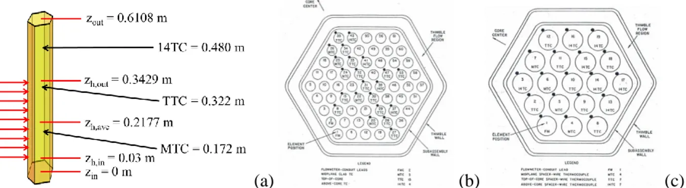
The EBR-II core was carefully instrumented and so it offers an ideal test bed for code validation. At least three sets of thermocouples (TC) are of particular interest here: 1) MTC (close to the middle of the heat region), 2) TTC (close to the outlet of the heated region) and 3) 14TC (close to the outlet of the bundle region), see Fig. 12a. In all cases standard spacer wires were replaced with TC wires, both in the XX09 and in the XX10 experimental HAs, see Fig. 12b, 12c and 4. These TCs provide a rather detailed map of some average temperature between Na and pin surface inside XX09 and XX10.
(a) (b) (c)
Fig. 12 Distribution of thermocouples in the EBR-II core: (a) axial location (red arrows indicate the power input region); (b) location inside XX09; (c) location inside XX10.
As seen in Sec. 2.1.1 and Fig. 6a, so far we used, for the benchmark purpose, the time dependent distribution of inlet Na temperature and mass flow rate among the HAs computed by RELAP5-3D© as BCs for FRENETIC. Moving now to the validation, it is reasonable to ask first to what extent RELAP5-3D© is able to reproduce the experimental results, as far as these BCs are concerned. A second question to be asked is to what extent the assumption of axially uniform power deposition made above (by both codes) is consistent with the experimental data. Only after all input uncertainties have been identified and their effects quantified by suitable sensitivity studies, we should be able to answer the question of the reliability of the model for inter-HA thermal coupling presently implemented in FRENETIC.
As far as the inlet temperature distribution is concerned, the temperature computed by RELAP5-3D© at the inlet of XX09 and XX10 (~ 626 K constant) compares well (not shown) with the measurement (varying between ~ 624 K and ~ 633 K) during the whole transient. The situation concerning the mass flow rate is more complicated, as only the total mass flow rate through one of the two main pumps (see Fig. 3a), namely #2, was measured, together with the mass flow rate at the inlet of the central hexagonal regions (excluding the thimble) of XX09 and XX10. The comparison between the total mass flow rate in pump #2 computed by RELAP5-3D© and measured is shown in Fig. 13, indicating that the agreement is qualitatively good. However, at intermediate times, the blind-phase RELAP5-3D© simulation overestimates up to ~ 100% the measured value, see the inset in Fig. 13. (It is also seen that, according to the simulation, the two pumps behave quite differently, as also stated in [11].)
Fig. 13 Computed vs. measured evolution of the mass flow rate in the two main pumps during the initial phase. The ratio between measured and computed values in pump #2, to be used as a scaling factor for the
FRENETIC boundary conditions (see text), is shown in the inset.
Therefore, while for XX09 and XX10 we have adopted the measured mass flow rate as BC, we compare below the measurements of the temperature evolution in XX09 and XX10 with the results computed by FRENETIC adopting as BC for the rest of the HAs the distribution of the mass flow rate computed by RELAP5-3D©, either as is or reduced by the instantaneous value of the ratio (measured)/(computed) total mass flow rate in pump#2.
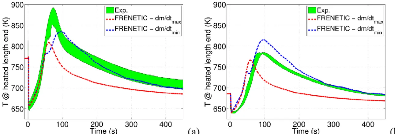
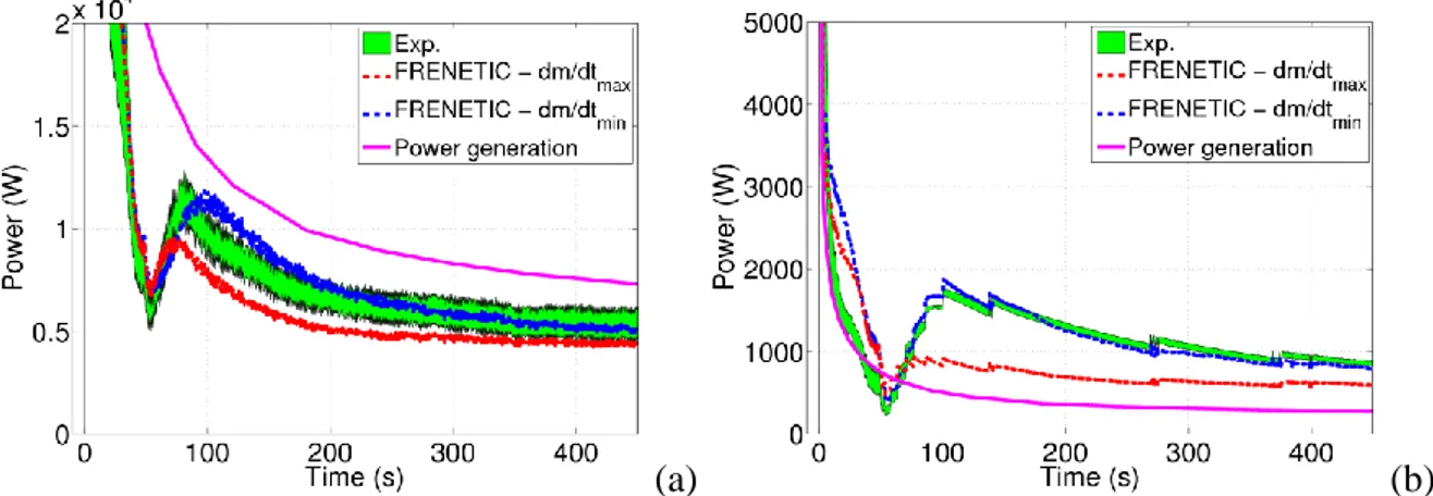
The measured temperature evolution at the end of the heated zone (the green colored band covers the range between minimum and maximum temperature) is compared with the FRENETIC simulation in Fig. 14 (the average between computed pin surface temperature and Na temperature is shown for consistency).
(a) (b)
Fig. 14 Computed vs. measured temperature evolution at the end of the heated zone: (a) XX09 HA; (b) XX10 HA. Computed values corresponding to different distributions of the coolant inlet mass flow rate on the core cross section: as computed by RELAP5-3D© (red curve); rescaled with the factor in the inset of Fig. 13 (blue
It is seen that the qualitative behavior of the measured temperature is reasonably reproduced by the simulation. While the initial temperature increase is similar for both mass flow rate distributions, since the scaling factor is very close to 1 in that phase of the transient, see the inset in Fig. 13, the later evolution is rather different in the two cases and presents features directly related to the strong variation of the scaling factor. It is to be noted that the measured temperature decrease is nicely bracketed by the two simulations.
Using the inlet mass flow rate (incompressible flow assumption) and the temperatures at the end of the heated length, it is possible to perform the calorimetry of the heated lengths of the XX09 and XX10 HAs (strictly speaking, excluding the thimble). The comparison between computation and measurement, reported in Fig. 15, shows a very good agreement. Notice that while in XX09 the coolant carries away less than the input power, because XX09 heats the colder neighboring HAs, the opposite is true for XX10, see also Fig. 6 and 8 above.
(a) (b)
Fig. 15 Computed vs. measured calorimetry of the central hexagonal channel of the experimental HAs: (a) XX09 HA; (b) XX10 HA.
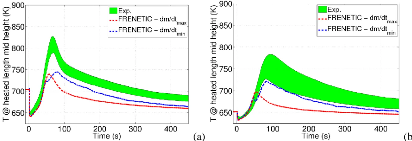
A last comparison between simulation and measurements is presented in Fig. 16, where the evolution of the coolant temperature at mid height of the heated region is reported. It is seen that the simulation is unable to bracket the measurement and underestimates the experimental coolant temperature. However, a comparison of the experimental traces in Fig. 15 and 16 shows that the temperature increase at mid height is ~ 2/3 of the total temperature increase across each channel, which is clearly incompatible with a uniform distribution of the input power along the HAs, as assumed here. An improvement of the model should require in this case a neutronic calculation giving a justifiable shape of the decay heat deposition along each HA.
(a) (b)
Fig. 16 Computed vs. measured temperature evolution at mid height of the heated zone: (a) XX09 HA; (b) XX10 HA. Different lines as defined in the caption of Fig. 14.
2.4
Conclusions and perspective
The results of the first qualification of the thermal-hydraulic module of the recently developed FRENETIC code in the case of a multi-assembly geometry have been presented. The computational domain includes a significant part of the EBR-II core, for a total of 127 assemblies of several different types.
First, a detailed comparison was performed between the results of FRENETIC and those of RELAP5-3D© (obtained during the blind phase of an international benchmark exercise), for both steady state and transient conditions, with particular reference to the Na temperature and to the pin surface temperature measured at different axial and radial locations in the core. Good agreement is shown between the results of the two codes, except in a few situations where, however, the discrepancies can be explained by differences in the two models.
The preliminary validation of the FRENETIC thermal-hydraulic module against EBR-II experimental data has also been presented. It was shown that, when all the uncertainties in the input parameters, and in particular in the boundary condition specifying the inlet mass flow rate distribution among the HAs, are taken into account, FRENETIC is able to reasonably bracket the experimental evolution of the coolant temperature at the outlet of the heated zone. While the EBR-II data are, to the best of our knowledge, the only available and relevant to a multi-assembly liquid-metal cooled geometry, the above-mentioned uncertainties are however too large in the case at hand to be able to definitely confirm the accuracy of the FRENETIC thermal-hydraulic model in a general multi-assembly geometry.
3
Development of the neutronic module
3.1 Introduction
The neutronic module of the FRENETIC code employs a coarse mesh nodal method to solve the multigroup neutron diffusion equations. Previously, the dynamics capabilities included only point kinetics or full inversion by way of the theta method. As a result of the work performed
during this year activity, the dynamics capabilities of the code are extended to include the quasi-static method. In order to implement the quasi-quasi-static capabilities, work is performed in two basic areas: the development and implementation of an adjoint solver and the development and implementation of multiple quasi-static solvers.
3.2 Adjoint capabilities of the neutronic module
In the nodal methods, one approach to the formulation of the adjoint problem in a manner which is mathematically consistent with the direct problem is to begin from the discretised (both in space and in energy) direct problem represented in matrix operator form
(1) with (2) (3) (4) (5)
In these definitions, the vector contains the node-averaged flux and flux moments, the vectors and represent the outgoing and incoming surface-averaged partial currents, respectively, the vector is the node-averaged source and the matrices and are the operators, the details of whose matrix structures are omitted from the present discussion.
The operators of the adjoint problem,
(6) with adjoint quantities denoted by a dagger, are obtained directly from definition with the auxiliary of a uniquely defined scalar product. The application of this process to the direct operators of Eqs. (4) and (5) yields for the corresponding adjoint operators
(7)
with the superscript indicating a matrix transpose and the two new matrices and containing nodal volumes and transverse surface areas, respectively. Thus, the nodal equations to be solved for the adjoint problem are known through the expansion of Eq. (6) using the definitions of Eqs. (7) and (8). Further elaboration of this approach and the implications in the context of a nodal method are addressed in [14].
3.3 Quasi-static capabilities of the neutronic module
The quasi-static method is based on the rationale that the neutron flux, solution of the balance equations in the presence of delayed emissions
(9)
may be factorised into the product of an amplitude function and a shape function, where the amplitude function follows the fastest evolving time scales and the shape function accounts for spatial and spectral variations whose temporal evolution occurs on a slower time scale:
(10)
with an appropriate projection procedure the original system of partial differential equations for the neutron flux and the delayed neutron precursors concentrations may be separated into two coupled systems of differential equations which can be solved separately for the unknowns on their respective time scales, the amplitude equation
(11)
and the shape function
The multiscale discretization of the time domain for quasi-static computations is shown in
Error! Reference source not found.. Three embedded time scales exist: the shape time step ∆tφ, the reactivity time step ∆tρ and the amplitude time step ∆tT, which respect the hierarchy ∆tφ≥∆tρ≥∆tT. The shape time steps are intended to resolve variations of the shape. The reactivity time steps account for variations of the integral kinetics parameters within a shape time step. Finally, the amplitude time steps are used to integrate the kinetics equations over an interval in which the shape and the kinetics parameters exhibit minor variations but the amplitude is evolving.
Fig. 17. Multiscale time discretisation for quasi-static computations. ∆tφ: shape time step; ∆tρ: reactivity time
step; ∆tT: amplitude time step.
The two basic algorithmic approaches of the quasi-static method are implemented: the improved quasi-static method (IQM) and the predictor-corrector quasi-static method (PCQM) [15]. The main difference between these two approaches is that the IQM solves the shape equation on the shape time step Δtφ, formula (12), to update the phase space neutron distribution, therefore having to deal with the non-linearity in such expression due to the presence of the amplitude and its derivative. The PCQM adopts a different approach, performing the shape update through the solution of the balance equation for the flux on Δtφ, therefore avoiding the problems connected to the non-linearity of the IQM implementation. In addition to the traditional versions of IQM and PCQM, modified versions of these two algorithms are implemented as an academic exercise, though they are not discussed herein [14, 15].
The integration of the amplitude equations across the shape time step, as well as the computation of the various derived quantities, is performed under the hypothesis the shape, the integral kinetics parameters, the fission source density per unit amplitude and the power density per unit amplitude vary linearly across the shape or reactivity time step.
Under the assumption that the shape varies linearly across the shape time step, the integral kinetics parameters are computed every reactivity time step using a shape function which is linearly interpolated across the shape time step and operators which are evaluated at the beginning and at the end of the reactivity time step. The actual values of the integral kinetics parameters that are used in the integration of the amplitude equations are their respective averages, obtained by assuming that each varies linearly across the reactivity time step. The amplitude equations are then solved exactly across the reactivity time step under the hypothesis that the integral kinetics parameters are constant on that same time step.
Within a shape time step, the spatial distribution of the delayed neutron precursors concentrations and the spatial distribution of the power are computed under the assumption that the fission source density per unit amplitude and the power density per unit amplitude, respectively, vary linearly across the reactivity time step, with their respective values at the beginning and at the end of the reactivity time step computed with a shape which is linearly interpolated across the shape time step. These assumptions are sufficient to ensure the continuity of the delayed neutron precursors concentrations and of the power contemporaneously with the amplitude.
These hypotheses are only truly applicable for PCQM, which has access to information about the shape at the end of the shape time step and therefore may make use of the assumed variation of the shape within the shape time step. Instead in IQM, the integration of the amplitude equations is completed prior to the update of the shape function, so only the shape function at the beginning of the shape time step can be used. Consequently, the power density is normally discontinuous at the interface of successive shape time steps, which is corrected by imposing a continuity condition on the total power, though at the cost of introducing a discontinuity on the amplitude.
The shape time step is adaptively managed (expanded or reduced) through an algorithm designed to control the permissible variation of the shape function over a shape time step. Reactivity time steps are adaptively managed as well.
In coupled neutronic/thermal-hydraulic calculations, the quasi-static algorithm is presently limited to shape time steps which are not greater than the neutronic/thermal-hydraulic coupling time step. The limitation is required only to accommodate features of the thermal-hydraulic module. However, the quasi-static solvers of the neutronic module are written with the envisagement that neutronic/thermal-hydraulic coupling is performed on reactivity time steps and therefore are already equipped to permit shape time steps which span multiple coupling time steps.
3.4 Representative results
The behaviour of the new features is assessed in the following two example transients. The first one is a pure neutronic transient, evaluated with the NE module working in stand-alone mode, while the second case presented has been calculated with the FRENETIC code, thus introducing the TH and NE coupling.
3.4.1 Compensated transient
The first test case involves a compensated transient applied to a small, non separable three-dimensional system. The reactor under consideration is shown in Fig. 18 and consists of a central hexagonal assembly surrounded by three full concentric rings of assemblies. The axis is equipartitioned into two zones, with the lower and the upper zone each comprised of the same material pattern, but out of phase by a rotation of 180 degrees and inverted in the central assembly. The two materials are described by two group diffusion theory parameters and a single delayed neutron precursor family while zero incoming partial current boundary conditions are imposed on all external surfaces of the system and the system is initially critical. A transient is initiated by instantaneously exchanging the materials. The choice of such configuration is of course not feasible in real-life systems, but it allows to consider a situation in which an initially critical system, after the transient initiator, still retains its critical condition and undergoes a strong spatial and spectral distortion of the neutron population, therefore testing the performance of the quasi-statics to follow these modifications. Test cases of this kind have been widely used in the literature in the development and testing of quasi-static algorithms [16].
Fig. 18. Initial configuration of the system studied for the compensated transient.
The time-dependent behaviour of the normalised total power computed with IQM and with PCQM is presented in Fig. 19, where the reference solution is the result of a full inversion of the problem using a fully implicit integration scheme on a fine discretisation of the time domain. These results demonstrate the typical features of the two quasi-static approaches, whose origin is in the shape function used to compute the power over the shape time step. Both methods regularly decrease the error as the shape time step is decreased; however, PCQM exhibits more favourable convergence than that of IQM. The time-dependent behaviour of the dynamic reactivity computed with IQM and with PCQM is presented in Fig. 20, with the reference value obtained by employing the normalised reference solution in the appropriate definition. It is observed that the ability to approximate the reference value is enhanced through the approximation of the shape function as being linear across the shape time step.
Fig. 19. Temporal evolution of the normalised total power for the compensated transient (finest PCQM discretisation indistinguishable from the reference solution).
Fig. 20. Temporal evolution of the dynamic reactivity for the compensated transient (finest PCQM discretisation indistinguishable from the reference solution).
3.4.2 Divergent transient with non-linear feedback
The second computational study involves a divergent transient applied to a lead-cooled fast reactor in three-dimensional, hexagonal-z geometry, as depicted in Fig. 21, modelled with three neutron energy groups and six delayed neutron precursors families. The transient follows from an instantaneous perturbation of the capture cross section for neutrons of energy group 2 in the upper half of the assembly number 3, equivalent to a step insertion of +111.90 pcm of static reactivity in a system for which the effective delayed neutron fraction is 338.82 pcm. Non linear feedback is introduced by rendering the cross sections temperature-dependent and performing a coupled neutronic/thermal-hydraulic analysis of the system.
Fig. 21. Geometrical configuration of the system studied for the divergent transient with non-linear feedback.
Results computed with IQM and PCQM are presented in Table 1 together with the reference solution, which is computed using a fully implicit, full inversion on a fine discretisation of the time domain (∆tφ=10-7
s). Quasi-static computations employ the adaptive time step selection algorithm in which the maximum permitted variation of the importance-weighted shape function across a shape time step is 10-2. Both quasi-static solutions are comparable to the reference solution as well as to each other; however, the fact that both IQM and PCQM produce essentially
the same results is a consequence of the maximum shape time step being limited to the neutronic/thermal-hydraulic time step (10-3 s).
Table 1. Time-dependendent power and reactivity for the divergent transient with nonlinear feedback (missing data correspond to reference results which are not computed for the entire duration of the transient).
Reference IQM PCQM
t [s] p(t)/p(0) [-] ρ(t) [pcm] p(t)/p(0) [-] ρ(t) [pcm] p(t)/p(0) [-] ρ(t) [pcm]
0.0000e+00 1.0000e+00 0.0000e+00 1.0000e+00 0.0000e+00 1.0000e+00 0.0000e+00 1.0000e-03 1.4930e+00 1.1179e+02 1.4930e+00 1.1179e+02 1.4930e+00 1.1179e+02 1.0000e-02 1.4961e+00 1.1167e+02 1.4961e+00 1.1167e+02 1.4961e+00 1.1167e+02 1.0000e-01 1.5232e+00 1.1035e+02 1.5233e+00 1.1035e+02 1.5233e+00 1.1035e+02 5.0000e-01 1.6079e+00 1.0439e+02 1.6080e+00 1.0439e+02 1.6080e+00 1.0439e+02 1.0000e+00 1.6670e+00 9.6779e+01 1.6671e+00 9.6777e+01 1.6670e+00 9.6777e+01
5.0000e+00 – – 1.7329e+00 5.3378e+01 1.7329e+00 5.3380e+01
1.0000e+01 – – 1.7264e+00 3.3773e+01 1.7264e+00 3.3776e+01
3.5 Conclusions
Adjoint and quasi-static capabilities are implemented in the neutronic module of the FRENETIC code. Representative results demonstrate functionality which is consistent with the presently implemented full inversion method, both in autonomous and coupled neutronic/thermal-hydraulic scenarios.
4
References
[1] USDOE Nuclear Energy Research Advisory Committee and the Generation IV International Forum, “A Technology Roadmap for Generation IV Nuclear Energy Systems,” GIF-002-00, 2002. [Online]. Available: http://www.gen-4.org/PDFs/GenIVRoadmap.pdf. [Accessed 28 February 2013].
[2] A. Alemberti, “The European lead fast reactor: design, safety approach and safety
characteristics,” Presented at the IAEA Technical Meeting on Impact of Fukushima Event on Current and Future FR Designs, Dresden, Germany, March 19-23, 2012. [Online]. Available: http://www.iaea.org/NuclearPower/Meetings/2012/2012-03-19-03-23-TM-NPTD.html. [Accessed 02 April 2014].
[3] A. Alemberti, D. De Bruyn, G. Grasso, L. Mansani, D. Mattioli and F. Roelofs, “The lead fast reactor e demonstrator (ALFRED) and ELFR design,” Presented at the International Conference on Fast Reactor and Nuclear Fuel Cycle (FR13), Paris, France, March 4-7, 2013. [Online]. Available: http://www.iaea.org/NuclearPower/Meetings/2013/2013- 03-04-03-07-CF-NPTD.html. [Accessed 31 January 2014].
[4] H. Aït Abderrahim, P. Baeten, D. De Bruyn and R. Fernandez, “MYRRHA – A multi-purpose fast spectrum research reactor,” Energy Conversion and Management, vol. 63, pp. 4-10, 2012.
[5] R. Bonifetto, S. Dulla, P. Ravetto, L. Savoldi Richard and R. Zanino, “A full-core coupled neutronic/thermal-hydraulic code for the modeling of lead-cooled nuclear fast reactors,”
Nuclear Engineering and Design, vol. 261, pp. 85-94, 2013.
[6] R. Bonifetto, S. Dulla, P. Ravetto, L. Savoldi Richard and R. Zanino, “Progress in multi-physics modeling of innovative lead-cooled fast reactors,” Transactions of Fusion Science
and Technology, vol. 61, pp. 293-297, 2012.
[7] R. Bonifetto, D. Caron, S. Dulla, P. Ravetto, L. Savoldi Richard and R. Zanino, Extension of
the FRENETIC code capabilities to the three-dimensional coupled dynamic simulation of LFR, Madrid (Spain): Presented at the 16th International Conference on Emerging Nuclear
Energy Systems (ICENES), May 26-30, 2013.
[8] R. Zanino, R. Bonifetto, A. Del Nevo and L. Savoldi Richard, “Benchmark and preliminary validation of the thermal-hydraulic module of the FRENETIC code against EBR-II data,” in
Transactions of the International Topical Meeting on Advances in Thermal Hydraulics,
Reno, NV (USA), June 15-19, 2014.
[9] R. Zanino, R. Bonifetto, A. Ciampichetti, I. Di Piazza, l. Savoldi Richard and M. Tarantino, “Validation of the thermal-hydraulic model in the FRENETIC code against data from the ENEA-CIRCE experiment,” Transactions of the American Nuclear Society, vol. 107, pp. 1395-1398, 2012.
[10] G. Golden and e. a. , “Evolution of thermal-hydraulics testing in EBR-II,” Nuclear
Engineering and Design, vol. 101, pp. 3-12, 1987.
[11] T. Sumner and T. Wei, “Benchmark Specifications and Data Requirements for EBR II Shutdown Heat Removal Tests SHRT 17 and SHRT 45R,” Nuclear Engineering Division Argonne National Laboratory, ANL-ARC-226-(Rev 1), May 31, 2012.
[12] The RELAP5-3D© Code Development Team, “RELAP5-3D© Code Manual Volume II: User’s Guide and Input Requirements,” INEEL-EXT-98-00834 Rev. 4.0, June 2012. [13] L. Savoldi Richard and R. Zanino, “M&M: multi-conductor mithrandir code for the
simulation of thermal-hydraulic transients in super-conducting magnets,” Cryogenics, vol. 40, pp. 179-189, 2000.
[14] D. Caron, S. Dulla and P. Ravetto, “Formulation and implementation of the quasi-static method for the solution of the neutron diffusion equation in the framework of a nodal method,” submitted to Annals of Nuclear Energy, 2014.
[15] S. Dulla, E. H. Mund and P. Ravetto, “The quasi-static method revisited,” Progress in
Nuclear Energy, vol. 50, pp. 908-920, 2008.
[16] J. B. Yasinsky and A. F. Henry, “Numerical experiments concerning space-time reactor kinetics behaviour,” Nuclear Science and Engineering, vol. 22, pp. 171-181, 1965.
5
Breve CV del gruppo di lavoro
Il gruppo di lavoro impegnato nell'attività opera presso il Dipartimento Energia del Politecnico di Torino ed è costituito da due professori ordinari (Piero Ravetto, fisica dei reattori nucleari e Roberto Zanino, impianti nucleari), due ricercatori confermati (Sandra Dulla, fisica dei reattori nucleari e Laura Savoldi, impianti nucleari), da un post-doc (Roberto Bonifetto) e da un dottorando (Dominic Caron) iscritto al I anno di Dottorato in Energetica.
Il gruppo ha una lunga esperienza nella ricerca nel campo dell’ingegneria nucleare, sia nel settore della fissione (S. Dulla e P. Ravetto) che nel settore della fusione (L. Savoldi e R. Zanino).
Nel settore della fissione l’attività ha riguardato lo sviluppo di metodi per il trasporto neutronico e per la dinamica dei reattori, in particolare per applicazioni ai sistemi nucleari avanzati (ADS e reattori innovativi). Nel settore della fusione il gruppo si è occupato dell’analisi termofluidodinamica di componenti di reattori a confinamento magnetico e in particolare dello sviluppo di codici per la modellazione del sistema dei magneti superconduttori e dell’applicazione di software CFD per l’analisi di blanket, first wall e vacuum vessel.
L’attività di Roberto Bonifetto comprende lo sviluppo e l’applicazione di codici per la modellazione di reattori nucleari a fissione (il codice presentato in questo lavoro) e a fusione (il codice 4C per l’analisi termofluidodinamica dei magneti superconduttori).
Nel lavoro presentato in questo rapporto sono state utilizzate le metodologie di simulazione termoidraulica messe a punto nel settore della fusione per lo sviluppo di un codice di multifisica per la dinamica di un reattore veloce refrigerato a piombo.
Maggiori dettagli e l'elenco delle pubblicazioni più recenti dei membri del gruppo si possono trovare sul sito Web del Politecnico di Torino:
http://porto.polito.it/view/creators/Ravetto=3APiero=3A000919=3A.html http://porto.polito.it/view/creators/Zanino=3ARoberto=3A001876=3A.html http://porto.polito.it/view/creators/Dulla=3ASandra=3A011663=3A.html http://porto.polito.it/view/creators/Savoldi=3ALaura=3A003575=3A.html http://porto.polito.it/view/creators/Bonifetto=3ARoberto=3A026979=3A.html