Attività di interconfronto tra codici di trasporto atmosferico per la preparazione e la risposta alle emergenze nucleari

(1)

(2)

dioattivi. I codici vengono confrontati su una singola simulazione di un possibile rilascio incidentale alla stazione frontaliera di Gösgen (CH), in condizioni meteorologiche sfavo-revoli per il territorio italiano.

In this work we present and compare the results obtained iwth three different codes (FLEXPART, CALPUFF and ldX) for the atmospheric dispersion of radioactive pollu-tants. The codes are compared on a single simulation of a possible incident release in the Gösgen (CH) nuclear power plant with weather conditions that are not favorable to the Italian territory.

(3)

Attività di interconfronto tra codici di

trasporto atmosferico per la preparazione e

la risposta alle emergenze nucleari

A. Cervone, A. Guglielmelli, C. Lombardo

ENEA FSN/SICNUC/SIN

13

th

February 2019

(4)

1 Codes for Atmospheric Dispersion of

Radioactive Material

Three different codes have been selected for the inter-comparison of atmospheric trans-port: FLEXPART, ldX and CALPUFF. These codes were selected because they are based on different modeling of the same physical phenomenon, with FLEXPART using the Lagrangian particle model, while ldX and CALPUFF rely on an Eulerian description of the dispersion.

1.1 FLEXPART

FLEXPART, an abbreviation for FLEXible PARTicle dispersion model, is a long-range

atmospheric transport code based on the Lagrangian model. In this approach, the

pollutant is modeled with a large number of particles that are followed in their evolution through the fixed grid that describes the atmospheric condition. A stochastic process is used to simulate the effect of the turbulence and to model transport, diffusion, wet and dry deposition, together with radioactive decay [1–3].

FLAXPART has been developed to work with different sets of meteorological weather data, such as ECMWF, GFS and WRF.

The main advantage of the Lagrangian approach is the complete absence of numerical diffusion, that is inherently introduced in Eulerian models. FLEXPART can perform forward and backward simulations in time, adding the possibility to recover an emission starting from some receptor value. FLEXPART is used in this capability also in the CTBTO for detecting and measuring of potential radioactive releases in the atmosphere.

1.2 ldX

ldX is a long-range, 3D, Eulerian atmospheric dispersion code developed and owned by the French Institute of Radiological Protection and Nuclear Safety (IRSN) for which the ENEA-FSN-SICNUC Division has signed a bilateral cooperation agreement. ldX is the IRSN reference code dedicate to evaluate on a regional scale (i.e., from some hundred up to several thousand kilometers) the radionuclides transport in the atmosphere. The code resolves the advection-diffusion fluid mechanics equations on an elementary volume and calculates the physical quantities homogeneously on the scale of an elementary computational cell with a dimension that depends on the spatial resolution chosen. ldX is capable of taking into account the radioactive filiation and decay during the transport, the wet scavenging and the dry deposition and allows defining finer physical models,

(6)

directly calling on more than 20 advanced meteorological parameters such as relative humidity or height of clouds [4]. The model implemented in ldX is analogous to that of Polair3D of the Polyphemus platform and has been validated against the European Tracer Experiment (ETEX), the Algeciras release, and the Chernobyl accident [5].

ldX uses Meteo France as weather data provider with two different geographical

do-mains: Arpege, with a resolution of 0.5◦, and Aladin, with a 0.1◦ spatial resolution.

1.3 CALPUFF

CALPUFF is an Eulerian-based code for the dispersion of pollutant in the atmosphere adopted by the U.S. Environmental Protection Agency (EPA) for long-range atmospheric dispersion [6]. CALPUF is organized in three main components: CALMET, a diagnostic three-dimensional meteorological model that manipulates the weather data; CALPUFF itself, the dispersion model for the pollutant; and CALPOST that manages the post-processing of the simulation results.

A list of applications on which CALPUFF has been successfully adopted is: near-field impacts in complex flow or dispersion situations; complex terrain; stagnation, inversion, recirculation, and fumigation conditions; overwater transport and coastal conditions; light wind speed and calm wind conditions; long-range transport; visibility assessments and Class I area impact studies; criteria pollutant modeling, including application to State Implementation Plan (SIP) development; secondary pollutant formation and par-ticulate matter modeling; buoyant area and line sources (e.g., forest fires and aluminum reduction facilities).

CALMET can operate with many weather data providers, including North American Mesoscale Model (NAM), NCEP, NOMADS and ECMWF.

A detailed description of the CALPUFF/CALMET simulations used in this report can be found in [7].

(7)

2 Simulation setup for code

inter-comparison

2.1 Release setup

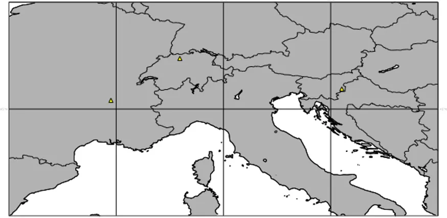
The selection of the emission date and place has been based on a statistical study that has covered 10 years (between 2002 and 2011) of simulated emissions for three of the closest nuclear power plants (NPPs) to the Italian border [8]. The NPPs are Krško (Slovenia), Saint-Alban (France) and Gösgen (Switzerland) and they are shown in Fig-ure 2.1. Among the 6000 simulated emissions for each NPP, it has been decided to pick one that would have a large impact on the Italian territory.

The selected NPP is Gösgen on the 16th of December 2011 at 19:30 UTC. The release is set to be of only a single isotope, Cs-137, with a value of 1e16 Bq over 1 hour (puff emission). This is a typical release for a PWR under severe accident conditions with sprays on and total containment failure [9]. The setup of the emission is summarized in Table 2.1.

2.2 Computational domain and time duration

The computational domain for the simulation has been set to the Italian territory,

cov-ered by a section of the Earth surface between 5◦ E and 20◦E in longitude, and between

35◦ N and 50◦ N in latitude. The resolution of the domain is different for each code, and

depends on the available weather data. For FLEXPART, the resolution is set to 0.25◦,

45°N 45°N

5°E 10°E 15°E

(8)

Location Gösgen Date 2011-12-16 Hour 19:30 UTC Duration 1h Isotope Cs-137 Quantity 1e16

Table 2.1: Release configuration.

for ldX the resolution is 0.4◦ and for CALPUFF the resolution is 0.5◦. The simulations

will be compared on the deposition maps over this whole territory.

The duration of the simulations is fixed to 4 days, since the largest part of the depo-sition occurs in this time frame, and only a residual part is omitted when looking at the deposition maps at the end of the simulations.

In addition to the final deposition maps, we will also compare the time evolution of the deposition in a single point of interest, the city of Trieste (only for CALPUFF and FLEXPART).

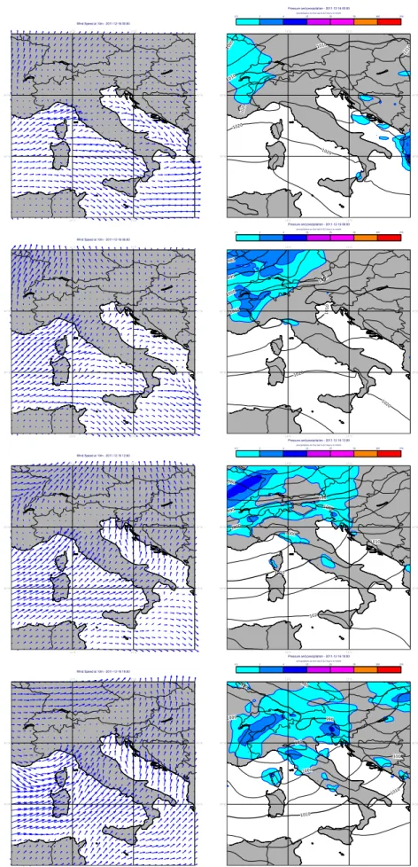
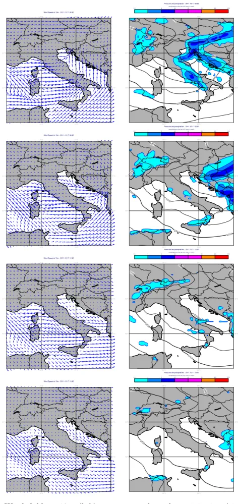
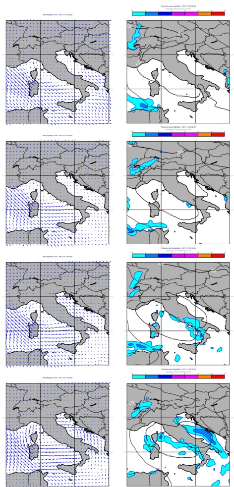
2.3 Weather conditions

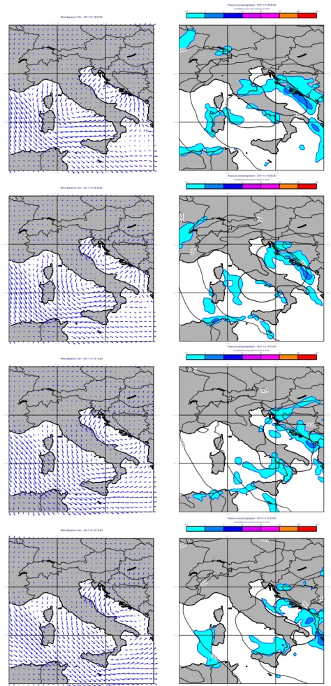
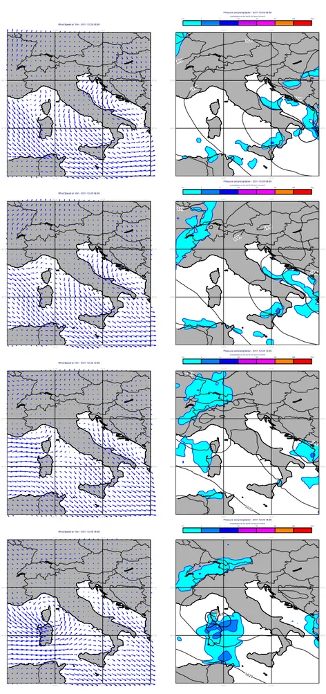
A selection of weather data for the simulation date can be seen in Figures 2.2-2.6 for the 5 days starting from the 2011-12-16 at 00:00 up to 2011-12-20 at 18:00. In particular, the maps show the wind (at 10 m from the ground) and the pressure isolines together with the total precipitation. The data have been obtained from ECMWF, using their ERA5

reanalysis database with a resolution of 0.25◦. In all the weather maps the Gösgen NPP

is indicated by a yellow triangle.

We can see that for the whole period the northern part of Italy is in quiet wind condition, while stronger winds can be seen on the Mediterranean sea west of Sardinia and north of the Alps. A low pressure zone develops on the 17th over the Adriatic sea and it slowly translates towards the Tyrrhenian sea in the following days. This conditions favor a stagnation of the radioactive cloud in the northern part of Italy, generating a higher deposition on the whole area.

Precipitations are very low over the whole period that has been considered. The highest values are registered on the first part of the 17th and 19th, but in any case they are located mainly over sea bodies, so they do not affect significantly the deposition on the Italian territory.

(9)

40°N 45°N 40°N 45°N 10°E 15°E 10°E 15°E Wind Speed at 10m - 2011-12-16 00:00 1000 1020 1020 1020 1010 1010 1010 40°N 45°N 40°N 45°N 10°E 15°E 10°E 15°E

Pressure and precipitation - 2011-12-16 00:00

precipitation on the last 6-12 hours in mm/h

0.5 2 4 10 25 50 100 250 40°N 45°N 40°N 45°N 10°E 15°E 10°E 15°E Wind Speed at 10m - 2011-12-16 06:00 980 1000 1000 1020 1020 990 1010 1010 40°N 45°N 40°N 45°N 10°E 15°E 10°E 15°E

0.5 2 4 10 25 50 100 250 40°N 45°N 40°N 45°N 10°E 15°E 10°E 15°E Wind Speed at 10m - 2011-12-16 12:00 990 990 1010 1010 980 1000 1000 1000 1020 40°N 45°N 40°N 45°N 10°E 15°E 10°E 15°E

0.5 2 4 10 25 50 100 250 40°N 45°N 40°N 45°N 10°E 15°E 10°E 15°E Wind Speed at 10m - 2011-12-16 18:00 980 1000 1000 1000 990 990 990 1010 1010 40°N 45°N 40°N 45°N 10°E 15°E 10°E 15°E

0.5 2 4 10 25 50 100 250

Figure 2.2: Wind field at 10m (left), pressure and total precipitation (right) on the 2011-12-16 at 00:00, 06:00, 12:00 and 18:00 (top to bottom).

(10)

40°N 45°N 40°N 45°N 10°E 15°E 10°E 15°E Wind Speed at 10m - 2011-12-17 00:00 1000 1000 1000 990 990 1010 1010 40°N 45°N 40°N 45°N 10°E 15°E 10°E 15°E

0.5 2 4 10 25 50 100 250 40°N 45°N 40°N 45°N 10°E 15°E 10°E 15°E Wind Speed at 10m - 2011-12-17 06:00 990 1010 1010 1010 1010 1000 1000 1000 40°N 45°N 40°N 45°N 10°E 15°E 10°E 15°E

0.5 2 4 10 25 50 100 250 40°N 45°N 40°N 45°N 10°E 15°E 10°E 15°E Wind Speed at 10m - 2011-12-17 12:00 990 1010 1010 1010 1000 1000 40°N 45°N 40°N 45°N 10°E 15°E 10°E 15°E

0.5 2 4 10 25 50 100 250 40°N 45°N 40°N 45°N 10°E 15°E 10°E 15°E Wind Speed at 10m - 2011-12-17 18:00 1000 1010 1010 1010 40°N 45°N 40°N 45°N 10°E 15°E 10°E 15°E

0.5 2 4 10 25 50 100 250

(11)

40°N 45°N 40°N 45°N 10°E 15°E 10°E 15°E Wind Speed at 10m - 2011-12-18 00:00 1010 1010 1010 1010 40°N 45°N 40°N 45°N 10°E 15°E 10°E 15°E

0.5 2 4 10 25 50 100 250 40°N 45°N 40°N 45°N 10°E 15°E 10°E 15°E Wind Speed at 10m - 2011-12-18 06:00 1010 1010 1010 40°N 45°N 40°N 45°N 10°E 15°E 10°E 15°E

0.5 2 4 10 25 50 100 250 40°N 45°N 40°N 45°N 10°E 15°E 10°E 15°E Wind Speed at 10m - 2011-12-18 18:00 1010 1020 40°N 45°N 40°N 45°N 10°E 15°E 10°E 15°E

0.5 2 4 10 25 50 100 250

(12)

40°N 45°N 40°N 45°N 10°E 15°E 10°E 15°E Wind Speed at 10m - 2011-12-19 00:00 1010 1010 1020 40°N 45°N 40°N 45°N 10°E 15°E 10°E 15°E

0.5 2 4 10 25 50 100 250 40°N 45°N 40°N 45°N 10°E 15°E 10°E 15°E Wind Speed at 10m - 2011-12-19 18:00 1010 1010 1020 1020 1020 1020 40°N 45°N 40°N 45°N 10°E 15°E 10°E 15°E

0.5 2 4 10 25 50 100 250

(13)

40°N 45°N 40°N 45°N 10°E 15°E 10°E 15°E Wind Speed at 10m - 2011-12-20 00:00 1010 1020 1020 1020 1020 40°N 45°N 40°N 45°N 10°E 15°E 10°E 15°E

0.5 2 4 10 25 50 100 250 40°N 45°N 40°N 45°N 10°E 15°E 10°E 15°E Wind Speed at 10m - 2011-12-20 18:00 1010 1020 40°N 45°N 40°N 45°N 10°E 15°E 10°E 15°E

0.5 2 4 10 25 50 100 250

(14)

3 Simulation results

This section summarizes the results obtained with the different codes described above. Details about the CALPUFF simulations can be found in [7]. The reference simulations that is used in the comparisons here is part of the set of simulations performed in [8], and a detailed description on the setup can be found in the reference.

The setup of the simulations follow the description of the previous section, that have been developed to minimize the differences among the codes. However, the mathemat-ical and numermathemat-ical models at the base of the codes are different, as FLEXPART is a Lagrangian based code, while CALPUFF and ldX are based on the Eulerian model. Furthermore, many modeling parameters are still inherently different among the codes, such as dry and wet deposition. This generates a relevant discrepancy in the results, that should be further investigated in order to understand what are the relevant differences to be addressed.

3.1 Deposited Cs-137 at the end of the simulation

40°N 45°N 40°N 45°N 10°E 15°E 10°E 15°E CALPUFF - fixed DP 1 10 100 220 500 1000 2000 5000 10000 20000 40°N 45°N 40°N 45°N 10°E 15°E 10°E 15°E CALPUFF - fixed vd 1 10 100 220 500 1000 2000 5000 10000 20000

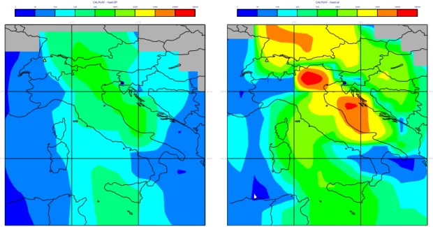
Figure 3.1: Comparison of CALPUFF final deposited Cs-137 in Bq/m2 with different

dry deposition models: fixed particle diameter (left) and fixed deposition

(15)

A clear example of the spread of the results can be seen in Figure 3.1, where we compare results obtained using the same code (CALPUFF) in the same configuration, with the only exception of the deposition model. In fact, CALPUFF implements two different strategies for the deposition: a model based on the diameter of the particles (shown on the left), and a simpler one where the deposition velocity is fixed by the user (on the right).

The same approach can be adopted in FLEXPART, using a deposition model based on multiple resistances (derived from the land use), or imposing a fixed deposition velocity, as is the case for CALPUFF and ldX. We can see from the CALPUFF example in Figure 3.1 that the deposited material absolute value is deeply influenced by the choice of the deposition model, while the pattern of the deposition is similar, as it is mainly influenced by the weather conditions.

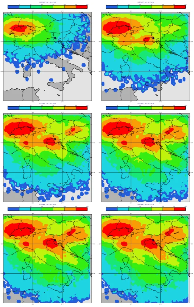
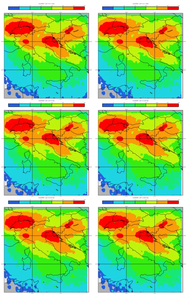
Figure 3.2 and Figure 3.3 show the time evolution of the deposition for the FLEXPART simulation. The first picture shows the deposited Cs-137 starting from 1:30 hours after the release, up to 16:30 after the relase in 3 hour intervals. We can clearly see that the deposited cloud reaches values relevant for radio-protection (an equivalent threshold of

220 Bq/m2 od Cs-220, see [8]) in Northern Italy already in the first instant displayed.

As the time progresses, higher values are registered inb the already-affected areas, with a relevant contamination that covers most of the peninsular Italy before the end of the first day from the release.

The second picture, Figure 3.3, shows the evolution of the deposition at later stages of the simulation, starting from about 20 hours after the release up to 4 days after with interval of 1 day between the last pictures. The deposition clearly does not change significantly after the first day. The zones with higher concentration are the ones near the release point, the upper part of the Adriatic sea (including Trieste), in the Piedmont region and over the eastern part of Slovenia and the western part of Hungary.

Different simulations have been performed to assess the dependency of the results on some parameters of the simulation such as: the number of particle released, the weather data resolution, the height of the release. None of this parameters generate significantly different patterns in the results obtained, with the exception of the deposition model described above.

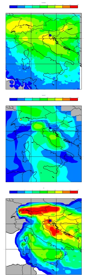
Figure 3.4 shows a comparison of the results obtained with the three codes on the same scale. It is clear that ldX predicts a much higher deposition than the other two codes, with a maximum of about 1 order of magnitude more than the others. The pattern of the deposition is, anyway, quite similar for the three codes.

it is noteworthy the highlight that FLEXPART predicts a quite uniform spread of deposition near the release point. This is not the case in CALPUFF, and especially in ldX, where the deposited material near the release point is mainly spread in the eastward direction. This is reflected also in the very low concentrations predicted by ldX and similarly by CALPUFF in the western part of Italy and in the south-east part of France.

(16)

40°N 45°N 40°N 45°N 10°E 15°E 10°E 15°E FLEXPART - 2011-12-16 21:00 1 10 100 220 500 1000 2000 5000 40°N 45°N 40°N 45°N 10°E 15°E 10°E 15°E FLEXPART - 2011-12-17 00:00 1 10 100 220 500 1000 2000 5000 40°N 45°N 40°N 45°N 10°E 15°E 10°E 15°E FLEXPART - 2011-12-17 03:00 1 10 100 220 500 1000 2000 5000 40°N 45°N 40°N 45°N 10°E 15°E 10°E 15°E FLEXPART - 2011-12-17 06:00 1 10 100 220 500 1000 2000 5000 40°N 45°N 40°N 45°N 10°E 15°E 10°E 15°E FLEXPART - 2011-12-17 09:00 1 10 100 220 500 1000 2000 5000 40°N 45°N 40°N 45°N 10°E 15°E 10°E 15°E FLEXPART - 2011-12-17 12:00 1 10 100 220 500 1000 2000 5000

Figure 3.2: Deposited Cs-137 in Bq/m2 at different times using FLEXPART. From

left to right and top to bottom: 2011-12-16 21:00, 2011-12-17 00:00,

2011-12-17 03:00, 2011-12-17 06:00, 2011-12-17 09:00, 2011-12-17 12:00.

(17)

40°N 45°N 40°N 45°N 10°E 15°E 10°E 15°E FLEXPART - 2011-12-17 15:00 1 10 100 220 500 1000 2000 5000 40°N 45°N 40°N 45°N 10°E 15°E 10°E 15°E FLEXPART - 2011-12-17 18:00 1 10 100 220 500 1000 2000 5000 40°N 45°N 40°N 45°N 10°E 15°E 10°E 15°E FLEXPART - 2011-12-17 21:00 1 10 100 220 500 1000 2000 5000 40°N 45°N 40°N 45°N 10°E 15°E 10°E 15°E FLEXPART - 2011-12-18 21:00 1 10 100 220 500 1000 2000 5000 40°N 45°N 40°N 45°N 10°E 15°E 10°E 15°E FLEXPART - 2011-12-19 21:00 1 10 100 220 500 1000 2000 5000 40°N 45°N 40°N 45°N 10°E 15°E 10°E 15°E FLEXPART - 2011-12-20 21:00 1 10 100 220 500 1000 2000 5000

Figure 3.3: Deposited Cs-137 in Bq/m2 at different times using FLEXPART. From

left to right and top to bottom: 2011-12-17 15:00, 2011-12-17 18:00,

2011-12-17 21:00, 2011-12-18 21:00, 2011-12-19 21:00, 2011-12-20 21:00.

(18)

40°N 45°N 40°N 45°N 10°E 15°E 10°E 15°E FLEXPART 1 10 100 220 500 1000 2000 5000 10000 100000 40°N 45°N 40°N 45°N 10°E 15°E 10°E 15°E CALPUFF 1 10 100 220 500 1000 2000 5000 10000 100000 40°N 45°N 40°N 45°N 10°E 15°E 10°E 15°E ldX 1 10 100 220 500 1000 2000 5000 10000 100000

Figure 3.4: Comparison of final deposited Cs-137 in Bq/m2 with FLEXPART

(left), CALPUFF (center) and ldX (right) on the same color scale.

(19)

3.2 Time evolution of deposited Cs-137 in Trieste

0 20 40 60 80 100

hours after the release 0 1000 2000 3000 4000 Bq / m2

Cumulated Cs-137 deposition in Trieste

FLEXPART CALPUFF, dp fixed CALPUFF, vd fixed

Figure 3.5: Comparison of the time evolution of the deposited Cs-137 in Trieste with FLEXPART and CALPUFF.

Figure 3.5 show a comparison of the time evolution of the deposited Cs-137 in the city of Trieste. This point on the grid has been chosen as a point of interest to assess the simulation results in their time evolution. The figure shows the results for the reference calculation using FLEXPART, together with two different simulations performed with CALPUFF, that differ in the deposition model, as seen already in Figure 3.1.

The results of the two CALPUFF simulation follow the same evolution, but differ by almost an order of magnitude in value. The first significant arrival of deposited Cs-137 is predicted to be after about 15 hours from the release, with a deposition rate that covers more than 80% of the final value in less than 5 hours. A second period of deposition is visible for both simulations at about 40 hours after the release and it lasts for about 10 hours.

In the case of FLEXPART, the arrival of the radioactive cloud happens earlier than CALPUFF, in fact the deposition starts immediately on the first output point (that is relative to 1.5 hours after the release). This is in accordance with what we have already observed in Figure ??. The deposition rate is smoother in FLEXPART, with almost all the deposition occurring in the first 20 hours. A very small bump on the deposited value can be seen also in FLEXPART at about 40 hours after the deposition, but is much smaller than the one we registered in CALPUFF.

(20)

4 Conclusions

The aim of this work is to have a first estimate of the differences among different modeling approaches and quantify the user effect that is inherently present in the setup of codes for atmospheric dispersion that give to its users many configuration parameters.

This exercise has shown the difficulties in properly matching configurations among different codes. Even in this well established setup, modeling features and configuration choices play a relevant role in the final output. On the contrary, weather data, at least in the re-analysis framework, seem to play a smaller role on the discrepancies obtained. A further in-depth analysis of the simulation setup is fostered, in order to understand the effect of the configuration choices on the simulation setup. An extension to different setups is also important to verify that the lessons learned by this exercise can be safely extended to a general framework.

Acknowledgements

The authors would like to acknowledge the use of ECMWF weather data for the simu-lations performed.

(21)

Bibliography

[1] A. Stohl, M. Hittenberger, and G. Wotawa. “Validation of the Lagrangian

parti-cle dispersion model FLEXPART against large-scale tracer experiment data”. In:

Atmospheric Environment 32.24 (1998), pp. 4245–4264.

[2] A. Stohl and D. J. Thomson. “A density correction for Lagrangian particle

disper-sion models”. In: Boundary-Layer Meteorology 90.1 (1999), pp. 155–167.

[3] A. Stohl et al. “The Lagrangian particle dispersion model FLEXPART version 6.2”.

In: Atmospheric Chemistry and Physics 5.9 (2005), pp. 2461–2474.

[4] Radiation Protection Division. Methodology used in IRSN nuclear accident cost

estimates in France. Tech. rep. PRP-CRI/SESUC/2014-132. IRSN.

[5] D. Quélo et al. “Validation of the Polyphemus platform on the ETEX, Chernobyl

and Algeciras cases”. In: Atmospheric Environment 41.26 (2007), pp. 5300–5315.

[6] US Environmental Protection Agency, Emissions Monitoring and Analysis Division.

A User’s Guide for the CALPUFF Dispersion Model. Tech. rep. Research Triangle

Park, N.C.: The Division, 1995.

[7] M. Giardina and P. Buffa. Transport and dispersion analyses of radioactive releases

following severe accident in Gösgen nuclear power plant. Tech. rep. CERSE-UNIPA

RL 4100/2019. CIRTEN.

[8] A. Guglielmelli, A. Cervone, and F. Rocchi. Sviluppo di algoritmi per la sintesi

in-tegrale dei risultati 2D di trasporto atmosferico finalizzati al ranking dei siti frontal-ieri. Tech. rep. ADPFISS-LP1-124. ENEA, 2018.

[9] A. Guglielmelli and F. Rocchi. “Evaluation of the radiological impact on the

Ital-ian territory of a severe nuclear accident at Krško NPP by means of a statistical methodology”. In: Proceedings of the 26th International Conference Nuclear Energy