Short-term and long-term health impacts of air pollution reductions from COVID-19 lockdowns in China and Europe: a modelling study

(1)

Supplementary appendix

This appendix formed part of the original submission and has been peer reviewed.

We post it as supplied by the authors.

Supplement to: Giani P, Castruccio S, Anav A, Howard D, Hu W, Crippa P. Short-term

and long-term health impacts of air pollution reductions from COVID-19 lockdowns

in China and Europe: a modelling study. Lancet Planet Health 2020; published online

Sept 22. http://dx.doi.org/10.1016/S2542-5196(20)30224-2.

(2)

1 Appendix to manuscript

Short- and long-term health impacts of air pollution reductions from COVID-19 lockdowns

in China and Europe

Paolo Giani

1

_{, Stefano Castruccio}

2

_{, Alessandro Anav}

3

_{, Don Howard}

4

_{, Wenjing Hu}

2

_{, Paola}

Crippa

1*

1_{Department of Civil and Environmental Engineering and Earth Sciences, University of Notre Dame, Notre Dame,}

IN, USA

2_{Department of Applied and Computational Mathematics and Statistics, University of Notre Dame, Notre Dame, IN,}

USA

3_{Climate Modeling Laboratory, ENEA, Italian National Agency for New Technologies, Energy and Sustainable}

Economic Development, CR Casaccia, Santa Maria di Galeria, Italy

4_{Department of Philosophy, University of Notre Dame, Notre Dame, IN, USA}

*Corresponding author: Paola Crippa, Department of Civil and Environmental Engineering and Earth Sciences,

(3)

2

EVIDENCE OF IMPROVED AIR QUALITY

The air quality index (AQI) for both China and Europe showed an overall improvement during the first quarter of 2020 as a response to the wide range of interventions implemented by national governments to contain the spread of COVID-19. In China, during the first 30 days following the shutdown (January 29 to February 29), 46% of the monitoring stations indicated a good to excellent air quality (AQI<=50) against 34% in the same period in 2019. For heavily to severely polluted air quality (AQI>100) during the same days, in 2020 only 2% of the stations indicated it against 7% in 2019. In some main cities in Europe, ground observations in the week of 16th_-22th_{March highlighted a}

sharp decrease, between 20% and 60%, of nitrogen dioxide (NO2) concentrations against the same week in 20191,2.

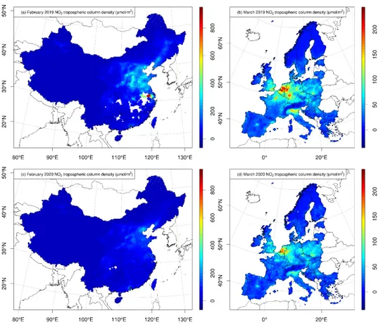
Similar conclusions can be drawn from satellite observations3_{which show a significant decrease in NO}₂_{concentrations}

in February and March as a result of the lockdown of most of the anthropogenic activities (Figure S1).

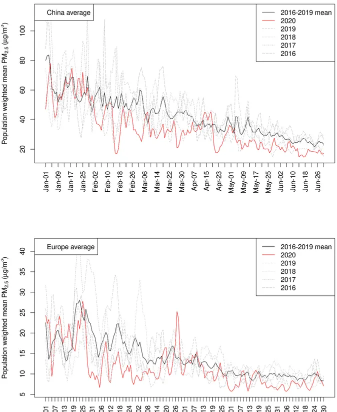
We analyze the differences between PM2.5 concentrations during post-outbreak period and the same period from

several previous years (2016-2019), to gain insights on the drivers of the air quality changes observed after COVID-19 outbreak. Even though interannual meteorological fluctuations can considerably affect PM2.5 concentrations4,5, the

observed decrease in PM2.5 throughout China cannot be ascribed to meteorological variations alone (Figure S2, Table

S4 and Table S7). The population-weighted mean PM2.5 during February-March 2020 is statistically lower than the

natural meteorological variability, as suggested by the p-values obtained by pairing 2020 concentrations with the same period in previous years (<<0.001, Table S7). This pattern is even more evident for Hubei province and other provinces highly impacted by lockdown measures (e.g. Zhejiang, Guangxi, Shaanxi, Henan, Shandong, Table S4). In Europe, the meteorological fluctuations play a more significant role in influencing 2020 concentrations. Although

population-weighted mean PM2.5 during the lockdown period (21 February-17 May) is also considerably lower than 2016-2019,

the statistical significance is weaker (Table S6). Exceptionally low PM2.5 concentrations have been observed during

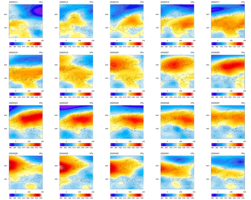
the second half of February and the beginning of March, whereas PM2.5 accumulated in most of central Europe toward

the end of March (Figure S3) because of westward transport from Eastern Europe and unfavorable meteorological conditions that suppressed the dispersion of pollutants (i.e., a high-pressure system was in place during March 21-March 28, Figure S4).

METHODS

PM2.5 OBSERVATIONS

Hourly PM2.5 observations for Mainland China, Hong Kong and Europe are retrieved from online archives of the

Ministry of Ecology and Environment (http://beijingair.sinaapp.com/), the Hong Kong Environmental Protection

Department (https://www.epd.gov.hk/epd) and the European Environment Agency

(http://www.eionet.europa.eu/aqportal), for 2016-2020. In our analysis, we only focus on European countries with at least one air quality station that reported PM2.5 data for 2020 on June 30. The list of European countries included in

our analysis is reported in Table S2. As of 2020, the Chinese network comprises more than 1,600 stations with valid data in the considered timeframe, while the European sites that to date have reported their data are approximately 1,000. PM2.5 daily means are computed at each site after preprocessing steps to ensure data quality. Specifically we

remove negative zero values, consecutive repeats of hourly PM2.5 concentrations for 4 or more hours, and daily average

when more than 30% of the hourly data in a day are zero/missing. For European data, we only consider data flagged as “valid” or “valid but below detection limit” in the database.

PM2.5 DAILY FIELD ESTIMATION

Our analysis combines different data sources to accurately estimate daily PM2.5 concentration fields in previous years

(2016-2019) and during the COVID-19 outbreak (2020). We employ a widely used Gaussian process regression interpolation technique (i.e., ordinary kriging6_{), with a deterministic mean trend surface modeled via a first order}

(4)

3

𝑧𝑧(𝑠𝑠) = 𝜇𝜇(𝑠𝑠) + 𝜀𝜀(𝑠𝑠), (1)

𝜇𝜇(𝑠𝑠) = 𝛽𝛽0+ 𝛽𝛽1𝑥𝑥(𝑠𝑠). (2)

In Equation (1), 𝑧𝑧(𝑠𝑠) is the target PM2.5 concentration field, 𝑠𝑠 is the spatial coordinate (two-dimensional), 𝜇𝜇(𝑠𝑠) is the

deterministic mean trend surface, 𝑥𝑥(𝑠𝑠) is the PM2.5 concentration given by the numerical model simulation and 𝜀𝜀(𝑠𝑠)

is a Gaussian field with a spherical covariance function6_{. The mean surface concentration is thus estimated by}

correcting the numerical model simulation with available observations and 𝜀𝜀(𝑠𝑠) is estimated via interpolation and added to the mean surface concentration with a kriging procedure. All the parameters in the model (𝛽𝛽0, 𝛽𝛽1 and the covariance function of 𝜀𝜀(𝑠𝑠)) are estimated on a daily basis to obtain daily PM2.5 concentration fields. This being a

stochastic model (i.e., 𝜀𝜀(𝑠𝑠) is a random field), we can efficiently obtain new random realizations of the process that preserve the main statistics of the estimated field for uncertainty quantification purposes7_{. All calculations are}

performed in log-space to avoid unphysical negative PM2.5 concentrations and to account for the inherent

log-normality of observed PM2.5 observed data.

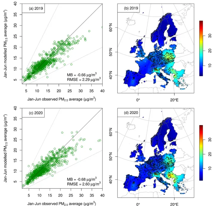
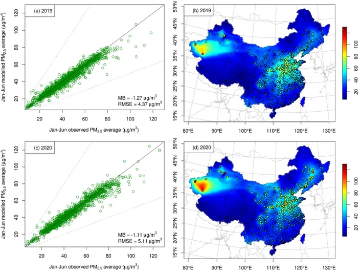
The methodology described here has been applied and validated previously in the literature and showed good skills in reproducing PM2.5 concentrations with cross-validation procedures8. For the present study, we report similar

cross-validation results for the first semester of 2019/2020 (Figure S6 and S7). The model is able to capture PM2.5

concentrations both in the typical range and during COVID-19 outbreak, as it is calibrated on observed data. Cross-validation mean bias is close to zero (-0.68 µg m-3_{for European data and -1.11 µg m}-3_{for Chinese data), and the}

magnitude of Root Mean Square Error (RMSE) is less than 20% of the average PM2.5 concentrations for both China

and Europe (Figure S6 and S7). The performance metrics reported herein indicate similar bias and lower RMSE than analogous regional scale studies which make use of satellite observations (e.g. Bai et al., 2019; Xue et al., 2019).

EMISSION SCENARIOS OF FUTURE ECONOMIC RECOVERY

Here we provide details on the four pathways of future economic recovery adopted in this work and how they impact PM2.5 concentrations.

1) Immediate resumption: this scenario assumes the lockdown interventions stop on April 1 in China and on May 17 in Europe, thus the annual PM2.5 concentrations are lower than prior years as a result of the PM2.5 decrease during the

lockdown periods, whereas for the remainder of the year PM2.5 levels return to their typical values (i.e., the average

between 2016 and 2019). We consider a 4-year average as typical concentrations to smooth out the meteorological variability.

2) Gradual resumption: this scenario is an analog for either a reaction/management of a prolonged pandemic crisis or reduced emissions associated with technological advances and/or changes to working habits and lifestyles (e.g., more remote working, reduced per capita energy consumptions). It assumes a progressive recovery in human activities, and thus a proportional increase of PM2.5 concentrations during April 1 – June 30 in China and during May 18 – August

18 in Europe. Each model grid cell is scaled by a coefficient calculated as the ratio of PM2.5 concentrations during the

post outbreak period and the same period during 2016-2019, on the first resumption day. The coefficients are then linearly increased every day until they reach 1 (i.e., typical concentrations) at the end of the three months recovery. 3) Fall outbreak: viral diseases are often characterized by seasonal outbreaks9,10_{, although it is still debated whether}

coronavirus will be weaker/latent during the summer in the Northern Hemisphere11_{. This scenario accounts for the}

possibility of a second coronavirus outbreak in the fall, which will require again social distancing measures, analogously to the one experienced in the first semester of 2020. We assume that PM2.5 concentrations sharply return

to typical levels on April 1 in China and May 18 in Europe, and a second outbreak between October to December occurs, in which concentrations are scaled by the same reduction coefficients calculated during the first outbreak. 4) Permanent lockdown: in the absence of evidence of effective control strategies other than social distancing and no available vaccine or effective medical treatments able to contain the pandemic spread, the extreme scenario of a

permanent lockdown for the whole of 2020 is considered. Typical PM2.5 concentrations are thus decreased by the

(5)

4

ASSESSMENT OF THE UNCERTAINTY FOR THE MORTALITY ESTIMATES

Confidence intervals of mortality estimates are estimated via Monte Carlo simulations8_{. We propagate uncertainty in}

PM2.5 fields, baseline mortality and RR parameters by sampling from the underlying probability distributions. The

uncertainty in PM2.5 fields is estimated through conditional simulations, i.e. random realizations of the Gaussian

(6)

5

Figure S1. Effect of NO2 emission reductions due to countries lockdown. Difference between monthly mean

NO2 tropospheric column density in 2020 and 2019 for (a-c) February in China and (b-d) March in Europe as

(7)

6

Figure S2. Comparison between population-weighted PM2.5 timeseries between 2020 and previous years, for

(8)

7

Figure S3. PM2.5 daily fields during March 24 – 31 2020 in Europe.

(9)

8

(10)

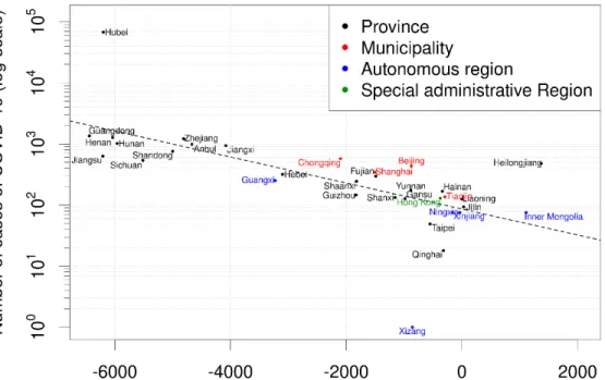
9

Figure S5. Number of COVID-19 cases for each province in China (top) and country in Europe (bottom), plotted against the long-term mortality difference due to PM2.5 variations between 2020 and 2016-2019 average

(11)

10

Figure S6. Cross-validation results PM2.5 mean concentrations for the first semester of 2019 (top) and 2020

(bottom) in Europe. PM2.5 concentration fields are reconstructed daily based on the methodology presented in

(12)

11

Figure S7. Cross-validation results PM2.5 mean concentrations for the first semester of 2019 (top) and 2020

(bottom) in China. PM2.5 concentration fields are reconstructed daily based on the methodology presented in

(13)

12

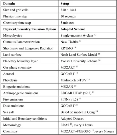
Table S1. Domain setup and physical and chemical schemes adopted for the WRF-Chem simulations presented in the work.

Domain Setup

Size and grid cells 330 × 1441 Physics time step 20 seconds Chemistry time step 5 minutes

Physics/Chemistry/Emission Option Adopted Scheme

Microphysics Single–moment 6–class 12

Cumulus Parameterization New Tiedtke 13

Shortwave and Longwave Radiation RRTMG 14

Land-surface Noah Land Surface Model 15

Planetary boundary layer Yonsei University Scheme 16

Gas phase chemistry MOZART 17

Aerosol GOCART 18

Photolysis Madronich F-TUV 19

Biogenic emissions MEGAN 20

Anthropogenic emissions EDGAR HTAP (v2.2) 21

Fire emissions FINN (v1.5) 22

Dust emissions GOCART 23

Sea salt Based on model in Gong 24

Initial and Boundary conditions Adopted Dataset Meteorology ERA5 25_{, every 3 hours}

(14)

13

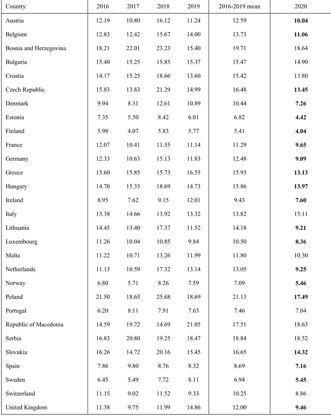
Table S2. Population weighted average of PM2.5 concentrations for all the European countries considered in

this work, during the lockdown period (February 21 – May 17) over the years 2016-2020. Values in bold indicate that the difference between PM2.5 concentrations in 2020 and the average of 2016-2019 are statistically

significant at 1% significance level (with a paired t-test on daily averages).

Country 2016 2017 2018 2019 2016-2019 mean 2020

Austria 12.19 10.80 16.12 11.24 12.59 10.04

Belgium 12.83 12.42 15.67 14.00 13.73 11.06

Bosnia and Herzegovina 18.21 22.01 23.23 15.40 19.71 18.64

Bulgaria 15.40 15.25 15.85 15.37 15.47 14.90 Croatia 14.17 15.25 18.66 13.60 15.42 13.80 Czech Republic 15.83 13.83 21.29 14.99 16.48 13.45 Denmark 9.94 8.31 12.61 10.89 10.44 7.26 Estonia 7.35 5.50 8.42 6.01 6.82 4.42 Finland 5.98 4.07 5.83 5.77 5.41 4.04 France 12.07 10.41 11.55 11.14 11.29 9.65 Germany 12.33 10.63 15.13 11.83 12.48 9.09 Greece 15.60 15.85 15.73 16.55 15.93 13.13 Hungary 14.70 15.33 18.69 14.73 15.86 13.97 Ireland 8.95 7.62 9.15 12.01 9.43 7.60 Italy 13.38 14.66 13.92 13.32 13.82 13.11 Lithuania 14.45 13.40 17.37 11.52 14.18 9.21 Luxembourg 11.26 10.04 10.85 9.84 10.50 8.36 Malta 11.22 10.71 13.26 11.99 11.80 10.30 Netherlands 11.13 10.59 17.32 13.14 13.05 9.25 Norway 6.80 5.71 8.26 7.59 7.09 5.46 Poland 21.50 18.65 25.68 18.69 21.13 17.49 Portugal 6.20 8.11 7.91 7.63 7.46 7.04 Republic of Macedonia 14.59 19.72 14.69 21.05 17.51 18.63 Serbia 16.83 20.80 19.25 18.47 18.84 18.52 Slovakia 16.26 14.72 20.16 15.45 16.65 14.32 Spain 7.86 9.80 8.76 8.32 8.69 7.16 Sweden 6.45 5.49 7.72 8.11 6.94 5.45 Switzerland 11.15 9.02 11.52 9.33 10.25 8.86 United Kingdom 11.38 9.75 11.99 14.86 12.00 9.46

(15)

14

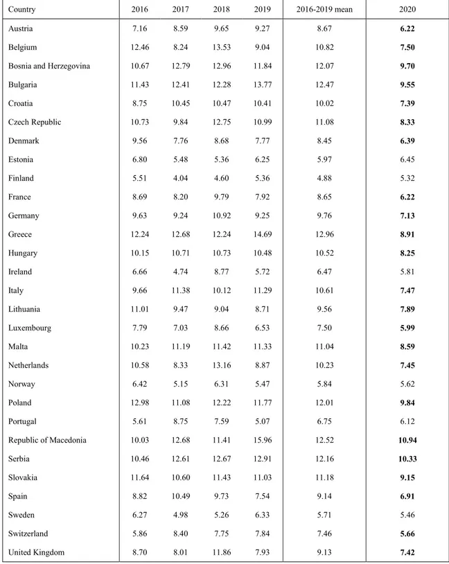
Table S3. Population weighted average of PM2.5 concentrations for all the European countries considered in

this work, during the resumption period (May 17 – June 30) over the years 2016-2020. Values in bold indicate that the difference between PM2.5 concentrations in 2020 and the average of 2016-2019 are statistically significant at 1% significance level (with a paired t-test on daily averages).

Country 2016 2017 2018 2019 2016-2019 mean 2020

Austria 7.16 8.59 9.65 9.27 8.67 6.22

Belgium 12.46 8.24 13.53 9.04 10.82 7.50

Bosnia and Herzegovina 10.67 12.79 12.96 11.84 12.07 9.70

Bulgaria 11.43 12.41 12.28 13.77 12.47 9.55 Croatia 8.75 10.45 10.47 10.41 10.02 7.39 Czech Republic 10.73 9.84 12.75 10.99 11.08 8.33 Denmark 9.56 7.76 8.68 7.77 8.45 6.39 Estonia 6.80 5.48 5.36 6.25 5.97 6.45 Finland 5.51 4.04 4.60 5.36 4.88 5.32 France 8.69 8.20 9.79 7.92 8.65 6.22 Germany 9.63 9.24 10.92 9.25 9.76 7.13 Greece 12.24 12.68 12.24 14.69 12.96 8.91 Hungary 10.15 10.71 10.73 10.48 10.52 8.25 Ireland 6.66 4.74 8.77 5.72 6.47 5.81 Italy 9.66 11.38 10.12 11.29 10.61 7.47 Lithuania 11.01 9.47 9.04 8.71 9.56 7.89 Luxembourg 7.79 7.03 8.66 6.53 7.50 5.99 Malta 10.23 11.19 11.42 11.33 11.04 8.59 Netherlands 10.58 8.33 13.16 8.87 10.23 7.45 Norway 6.42 5.15 6.31 5.47 5.84 5.62 Poland 12.98 11.08 12.22 11.77 12.01 9.84 Portugal 5.61 8.75 7.59 5.07 6.75 6.12 Republic of Macedonia 10.03 12.68 11.41 15.96 12.52 10.94 Serbia 10.46 12.61 12.67 12.91 12.16 10.33 Slovakia 11.64 10.60 11.43 11.03 11.18 9.15 Spain 8.82 10.49 9.73 7.54 9.14 6.91 Sweden 6.27 4.98 5.26 6.33 5.71 5.46 Switzerland 5.86 8.40 7.75 7.84 7.46 5.66 United Kingdom 8.70 8.01 11.86 7.93 9.13 7.42

(16)

15

Table S4. Population weighted average of PM2.5 concentrations for all provinces in China, during the lockdown

period (February 1 – March 31) over the years 2016-2020. Values in bold indicate that the difference between PM2.5 concentrations in 2020 and the average of 2016-2019 are statistically significant at 1% significance level

(with a paired t-test on daily averages).

Province 2016 2017 2018 2019 2016-2019 mean 2020 Anhui Province 68.37 71.86 60.37 63.91 66.13 42.91 Beijing Municipality 64.24 65.93 68.27 52.48 62.73 47.39 Chongqing Municipality 61.15 48.45 47.26 42.59 49.86 40.25 Fujian Province 35.27 33.17 33.29 26.44 32.04 23.31 Gansu province 41.48 44.37 44.99 35.33 41.54 31.49 Guangdong Province 36.63 37.78 38.98 25.52 34.73 22.67

Guangxi Zhuang Autonomous Region 45.84 42.94 49.32 29.47 41.89 29.36

Guizhou Province 43.17 34.92 42.01 27.76 36.97 29.84

Hainan Province 24.03 21.85 24.43 15.41 21.43 13.31

Hebei Province 68.72 79.13 77.10 71.00 73.99 49.73

Heilongjiang Province 38.78 38.18 41.79 53.21 42.99 35.24

Henan Province 77.69 82.44 76.00 80.77 79.22 52.73

Hong Kong Special Administrative Region 29.13 29.17 27.91 19.90 26.53 19.20

Hubei Province 69.18 61.20 57.52 53.30 60.30 38.25

Hunan Province 58.47 47.92 50.53 39.47 49.10 33.30

Inner Mongolia Autonomous Region 36.75 35.20 36.40 33.47 35.46 30.39

Jiangsu Province 68.31 60.76 57.13 58.55 61.19 37.14

Jiangxi Province 50.69 47.02 43.62 29.27 42.65 25.87

Jilin Province 44.99 50.77 47.05 54.39 49.30 34.52

Liaoning Province 49.84 58.93 54.90 56.14 54.95 40.43

Ningxia Hui Autonomous Region 50.00 47.98 46.47 38.36 45.70 34.09

Qinghai Province 44.74 39.47 40.49 30.78 38.87 26.34 Shaanxi Province 60.57 70.01 66.24 62.44 64.81 48.32 Shandong Province 75.82 70.32 61.00 73.00 70.03 47.47 Shanghai Municipality 53.84 47.80 43.34 46.59 47.89 28.69 Shanxi Province 55.25 70.12 69.98 61.23 64.15 45.01 Sichuan Province 59.02 50.02 53.69 43.12 51.46 39.69 Taiwan Province 34.20 31.41 29.07 24.81 29.87 23.70 Tianjin Municipality 65.89 75.42 70.48 66.13 69.48 50.25

Tibet Autonomous Region 23.29 18.78 17.52 11.72 17.83 10.09

Xinjiang Uygur Autonomous Region 112.18 79.01 74.27 72.82 84.57 72.10

Yunnan Province 37.84 35.19 38.46 29.46 35.24 32.85

(17)

16

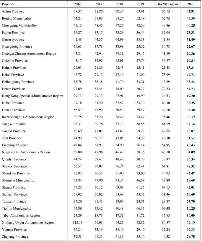
Table S5. Population weighted average of PM2.5 concentrations for all provinces in China, during the

resumption period (April 1 – June 30) over the years 2016-2020. Values in bold indicate that the difference between PM2.5 concentrations in 2020 and the average of 2016-2019 are statistically significant at 1%

significance level (with a paired t-test on daily averages).

Province 2016 2017 2018 2019 2016-2019 mean 2020 Anhui Province 41.61 47.63 41.42 33.33 41.00 28.47 Beijing Municipality 53.90 49.78 50.70 37.95 48.08 31.10 Chongqing Municipality 37.65 31.42 28.54 25.67 30.82 24.57 Fujian Province 25.41 23.64 26.29 22.35 24.42 18.50 Gansu province 28.63 30.32 32.98 24.79 29.18 21.92 Guangdong Province 25.08 26.08 25.31 18.31 23.70 17.13

Guangxi Zhuang Autonomous Region 27.83 28.21 27.22 22.82 26.52 21.97

Guizhou Province 26.15 24.07 25.10 19.99 23.83 19.86

Hainan Province 14.57 13.69 13.55 12.12 13.48 11.26

Hebei Province 50.54 52.41 45.51 37.17 46.41 31.51

Heilongjiang Province 23.30 26.99 25.64 18.82 23.69 24.59

Henan Province 48.35 49.58 42.75 37.00 44.42 32.24

Hong Kong Special Administrative Region 17.56 19.08 17.70 14.25 17.15 12.94

Hubei Province 36.74 38.08 34.57 30.80 35.05 26.82

Hunan Province 33.00 30.17 29.69 26.66 29.88 25.29

Inner Mongolia Autonomous Region 28.22 27.93 27.79 23.26 26.80 20.92

Jiangsu Province 43.15 43.00 42.89 33.39 40.61 31.71

Jiangxi Province 30.25 33.73 29.21 25.20 29.60 23.17

Jilin Province 27.45 30.30 28.40 22.30 27.11 32.07

Liaoning Province 35.32 34.65 32.72 29.07 32.94 29.62 Ningxia Hui Autonomous Region 33.16 36.12 37.59 28.51 33.84 24.29

Qinghai Province 31.64 25.51 32.79 23.56 28.37 20.66 Shaanxi Province 35.66 36.83 36.12 32.23 35.21 26.78 Shandong Province 52.94 49.30 40.49 36.94 44.92 33.82 Shanghai Municipality 45.04 36.93 38.30 30.55 37.71 31.04 Shanxi Province 40.06 43.07 43.38 34.26 40.19 30.46 Sichuan Province 36.62 32.26 31.17 26.32 31.59 25.92 Taiwan Province 24.07 22.18 22.66 19.72 22.16 16.87 Tianjin Municipality 54.39 54.83 47.49 39.96 49.17 35.13

Tibet Autonomous Region 21.12 15.95 16.68 11.47 16.30 9.88

Xinjiang Uygur Autonomous Region 50.56 39.50 54.12 31.20 43.84 39.16

Yunnan Province 24.17 24.58 24.29 24.92 24.49 20.75

(18)

17

Table S6. P-values of paired t-test to compare daily population weighted PM2.5 mean in different years, during

the lockdown period (February 21 – May 17) in Europe.

2016 2017 2018 2019 2020 2016 - 0.28 0.00089 0.71 0.00063 2017 - - 0.00018 0.30 0.0040 2018 - - - 0.0020 <0.0001 2019 - - - - 0.00082 2020 - - - - -

(19)

18

Table S7. P-values of paired t-test to compare daily population weighted PM2.5 mean in different years, during

the lockdown period (February 1 – March 31) in China. Differences between pairwise years 2016-2019 are not statistically significant at a 5% significance level (except for the pair 2016-2019, which is weakly significant), whereas a strongly significant difference is observed between 2020 and all previous years.

2016 2017 2018 2019 2020 2016 - 0.42 0.090 0.043 <0.0001 2017 - - 0.22 0.14 <0.0001 2018 - - - 0.84 <0.0001 2019 - - - - <0.0001 2020 - - - - -

(20)

19 Additional references

1 EEA. Air pollution goes down as Europe takes hard measures to combat coronavirus,

2020).

2 Tobías, A. et al. Changes in air quality during the lockdown in Barcelona (Spain) one

month into the SARS-CoV-2 epidemic. Science of The Total Environment, 138540 (2020).

3 Dutheil, F., Baker, J. S. & Navel, V. COVID-19 as a factor influencing air pollution?

Environmental Pollution

263, 114466, doi:https://doi.org/10.1016/j.envpol.2020.114466

(2020).

4 Wang, X., Dickinson, R. E., Su, L., Zhou, C. & Wang, K. PM2.5 Pollution in China and

How It Has Been Exacerbated by Terrain and Meteorological Conditions. Bulletin of the

American Meteorological Society

99, 105-119, doi:10.1175/bams-d-16-0301.1 (2018).

5 Chin, M. Dirtier air from a weaker monsoon. Nature Geoscience

5, 449-450,

doi:10.1038/ngeo1513 (2012).

6 Cressie, N. Statistics for Spatial Data. (Wiley, 1993).

7 Yang, Y. et al. Uncertainty assessment of PM

2.5

contamination mapping using

spatiotemporal sequential indicator simulations and multi-temporal monitoring data.

Scientific reports

6, 1-13 (2016).

8 Giani, P., Anav, A., De Marco, A., Zhaozhong, F. & Crippa, P. Exploring sources of

uncertainty in premature mortality estimates from fine particulate matter: the case of China.

Environmental Research Letters (2020).

9 Lowen, A. C. & Steel, J. Roles of Humidity and Temperature in Shaping Influenza

Seasonality. Journal of Virology

88, 7692-7695, doi:10.1128/jvi.03544-13 (2014).

10 Dushoff, J., Plotkin, J. B., Levin, S. A. & Earn, D. J. D. Dynamical resonance can account

for seasonality of influenza epidemics. Proceedings of the National Academy of Sciences

of the United States of America

101, 16915-16916, doi:10.1073/pnas.0407293101 (2004).

11 Luo, W. et al. The role of absolute humidity on transmission rates of the COVID-19

outbreak. medRxiv, 2020.2002.2012.20022467, doi:10.1101/2020.02.12.20022467 (2020).

12 Hong, S. Y. & J. Lim, J. O. The WRF single-moment 6-class microphysics scheme (WSM6).

Vol. 42 (2006).

13 Tiedtke, M. A Comprehensive Mass Flux Scheme for Cumulus Parameterization in

Large-Scale Models. Monthly Weather Review

117, 1779-1800,

doi:10.1175/1520-0493(1989)117<1779:acmfsf>2.0.co;2 (1989).

14 Iacono, M. J. et al. Radiative forcing by long-lived greenhouse gases: Calculations with

the AER radiative transfer models. Journal of Geophysical Research: Atmospheres

113,

doi:10.1029/2008jd009944 (2008).

(21)

20

15 Chen, F. & Dudhia, J. Coupling an Advanced Land Surface–Hydrology Model with the

Penn State–NCAR MM5 Modeling System. Part I: Model Implementation and Sensitivity.

Monthly Weather Review

129, 569-585,

doi:10.1175/1520-0493(2001)129<0569:caalsh>2.0.co;2 (2001).

16 Hong, S. Y., Noh, Y. & Dudhia, J. A new vertical diffusion package with an explicit

treatment of entrainment processes. Monthly Weather Review

134, 2318-2341,

doi:10.1175/mwr3199.1 (2006).

17 Emmons, L. K. et al. Description and evaluation of the Model for Ozone and Related

chemical Tracers, version 4 (MOZART-4). Geosci. Model Dev.

3, 43-67,

doi:10.5194/gmd-3-43-2010 (2010).

18 Chin, M., Rood, R. B., Lin, S.-J., Müller, J.-F. & Thompson, A. M. Atmospheric sulfur

cycle simulated in the global model GOCART: Model description and global properties.

Journal of Geophysical Research: Atmospheres

105, 24671-24687,

doi:10.1029/2000jd900384 (2000).

19 Madronich, S. Photodissociation in the atmosphere: 1. Actinic flux and the effects of

ground reflections and clouds. Journal of Geophysical Research: Atmospheres

92,

9740-9752 (1987).

20 Guenther, A. B. et al. The Model of Emissions of Gases and Aerosols from Nature version

2.1 (MEGAN2.1): an extended and updated framework for modeling biogenic emissions.

Geosci. Model Dev.

5, 1471-1492, doi:10.5194/gmd-5-1471-2012 (2012).

21 Janssens-Maenhout, G. et al. HTAP_v2.2: a mosaic of regional and global emission grid

maps for 2008 and 2010 to study hemispheric transport of air pollution. Atmos. Chem.

Phys.

15, 11411-11432, doi:10.5194/acp-15-11411-2015 (2015).

22 Wiedinmyer, C. et al. The Fire INventory from NCAR (FINN): a high resolution global

model to estimate the emissions from open burning. Geosci. Model Dev.

4, 625-641,

doi:10.5194/gmd-4-625-2011 (2011).

23 Ginoux, P. et al. Sources and distributions of dust aerosols simulated with the GOCART

model. Journal of Geophysical Research: Atmospheres

106, 20255-20273,

doi:10.1029/2000jd000053 (2001).

24 Gong, S. L. A parameterization of sea-salt aerosol source function for sub- and

super-micron particles. Global Biogeochemical Cycles

17, doi:10.1029/2003gb002079 (2003).

25 C3S. (ed Copernicus Climate Change Service)

(https://cds.climate.copernicus.eu/cdsapp#!/home, Copernicus Climate Change Service

Climate Data Store (CDS), 2017).

26 Bai, K., K. Li, N.-B. Chang, and W. Gao (2019), Advancing the prediction accuracy of

satellite-based PM2. 5 concentration mapping: A perspective of data mining through in situ

PM2. 5 measurements, Environmental Pollution, 254, 113047

(22)