Chapter 3
The wheel suspension model
When we talk about suspensions geometry it means the broad subject of how the unsprung mass of a vehicle is connected to the sprung mass. These connections not only dictate the path of relative motion but they also control the forces that are transmitted between them. In particular, the steering torque is strongly affected by the suspension layout and, for an accurate description of it, the introduction of a suspension model is required. Furthermore, suspensions have both a direct effect on the vehicle dynamics because of the increased sprung mass mobility, and an indirect one, because they change the orientation of the wheel with respect to the road, affecting the tyres answer. To take into account of the above mentioned aspects a suspension model is developed in this chapter, that allows to investigate the influence of the suspension travel on the steering torque feedback. Talking about race car [14], F1 and Formula SAE in particular being the object of this
work, the most common suspension is a five links independent suspension with double wishbone (A-arm) and tie rod: a description of it is given in the first paragraph of this chapter and will be the modelled suspension type in this work. In the real word the components that supply the restraints are not “perfect” in the sense of infinite stiffness but in this study any effect of compliance or deflections of the structural components will be neglected and the wheel suspension is modeled as a multibody model with rigid components connected by several joints.
3.1 The Suspension geometry
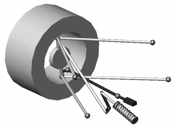
It is known that a body has six degrees of freedom (DOF) in a three-dimensional word. That means that also a wheel moving relatively to the vehicle body needs three components of linear motion and three components of rotational motion to completely define the relative position. For an independent suspension the assemblage of control arms is intended to control the motion of the wheel relative to the car body in a single fixed path (1 DOF). Using straight links with rod ends (spherical joints) the required five restraints can be provided with five of them: two links for both upper and lower A-arm and one for the tie rod. Note that for the front suspension we have an additional degree of freedom (steer rotation degree) but only when it is demanded from the steering system. The five links independent suspension called SLA is the most common geometry for a race car [14]. In the figure here below, the SLA front left suspension of the Leeds Formula Student car is shown.
Figure 3.1: SLA double wishbone suspension.
As someone said this kind of suspension is the choice of designers without question for its ability to meet desired performance objectives with minimum compromise. SLA stands for short-long arm and it’s a generic name for a family of suspensions that have upper and lower control arms with the upper shorter than the lower. This geometry can be used for both front and rear suspension with the only difference that, in the rear, the toe link is grounded to the chassis instead of attaching to a rack.
3.2 The model
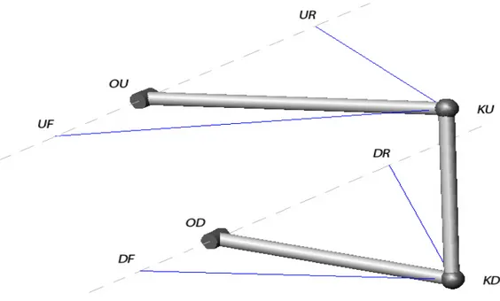
For an accurate description of the wheel suspension state, the wheel suspension can be modeled as a multibody model with rigid components connected by several joints. If we look at figure 3.2 we can easily recognize that a SLA suspension is a three dimensional four bar mechanism [15].
Figure 3.2: Three dimensional four bar mechanism
In fact, if we look for example at the lower control arm LCA, it is cinematically equivalent to a single bar rotating around a fixed axle identified by the position of the relative pick-up points DFand DR. The point around witch the bar rotates is the
Lower Control Arm inner pivot OD and it is the projection of the lower ball joint KD on the already mentioned axle. The same can be said of course for the upper
link OD-OU, the two cranks OD-KD and OU-KU rotating around their two revolute
joints and the coupler KD-KU connected to the cranks by two spherical joints.
In planar kinematics the four-bar, with the properties of the coupler curve (points velocity, acceleration… etc ), is a well known subject of study [16], but in spatial kinematics things become harder because of the third dimension. That’s why normally a 2D look-up table approach is used in studying the kinematics of such a suspension. I didn’t known that I could be able to find a mathematical expression for the path of the wheel center and its velocity (chapters 3 and 6). I found it interesting and I wanted to proceed on that way, that can be also the starting point for further investigation of the influence of the wheel-suspension parameter (ex: pick-up points position, camber and caster angle) on the wheel path and on the transfer of the wheel forces to the rack. In order to investigate the mechanism number of degrees of freedom we apply Grüblers formula [17]. It says that a rigid body has six degrees of freedom, and the total number of freedoms must be reduced by the number of constraints. The number of constrains is five for a revolute pairs and three for a spherical one. So the four-bar has 3×6-2×5-2×3=2 degrees of freedom, including the rotation of the coupler around its own axis (that is what allows the wheel to steer). To fully describe the motion performed by the suspension and then the path of the wheel center, we need to decide witch quantities will control the motion. They are:
• the λ angle experienced by the lower control arm with respect to the horizontal position , positive when the arm moves upwards.
• the yrack displacement that control the coupler rotation ( steering angle) via
Of course this is valid for the front suspension. The rear suspension still has the trackrod but there isn’t a rack. The trackrod is grounded to the chassis by a spherical joint and the suspension looses its second degree and has just the first one.
Starting from the position of the four pick-up points UF, UR, DF and DR (those also may not result in two parallel axes) we need to define two local axis systems: one for the UCA and one for the LCA. These axis systems are chosen in the way that they have their x_axis coincident respectively with the rotational UCA and LCA axle, the y_axis is always parallel to the ground, pointing to the left as the body axis system, and the z_axis comes as a consequence (see the Matlab file in appendix for more details). The centers are located on the inner pivot points OU
and OD. We call these two axis systems respectively ∑TU and ∑TD. Once identified
these two coordinate systems, are known the two rotational matrices TU and TD to
pass from the body axis system ∑''' to ∑TU and ∑TD. They are (see paragraph 1.3)
the coordinates of the vectors of the local axis system respect to the body axis system ∑'''. With respect to their local axis system the path of the ball joints KU
and KD can be expressed by the following equations in parametric form:
⎥ ⎥ ⎥ ⎦ ⎤ ⎢ ⎢ ⎢ ⎣ ⎡ ⋅ ⋅ = ) sin( ) cos( 0 τ τ Lu Lu KUTU (3.1)
where Lu is the UCA length and τ is the angle between the arm and the y_axis of
⎥ ⎥ ⎥ ⎦ ⎤ ⎢ ⎢ ⎢ ⎣ ⎡ ⋅ ⋅ = ) sin( ) cos( 0 λ λ Ld Ld KDTD (3.2)
where Ld is the LCA length and λ is the angle between the arm and the y_axis of
∑TD. As already mentioned λ will be the independent variable of the motion and τ will be expressed as a function of λ. Making use of rotational matrices TU and TD
we can write the path equation of the lower ball joint KD with respect to the ∑TU axis system. It reads:
KDTU = TU T · [TD · KDTD + ( OD - OU )] (3.3)
where TU T is the rotational matrix transpose of ∑TU and TD is the rotational matrix
of ∑TD. In the equation the quantities OD and OU represent the vectors which components are the coordinate of the inner pivots relatively to the body axis system. Writing the equation of the distance between the two points KU and KD in
the ∑TU coordinate system and making it equal to the knuckle length d (eq.3.4) we can easily obtain the linear trigonometric equation (3.5) in sin(τ) and cos(τ).
(3.4)
(
)
2 2. d KD KUTU − TD = A( )
λ ⋅cos( ) ( )
τ +Bλ ⋅sin( ) ( )
τ +C λ =0 (3.5)with
( )
( )
2 2 2 3 2 2 2 d Lu KD C KD Lu B KD Lu A TU TU TU − + = ⋅ ⋅ − = ⋅ ⋅ − = (3.6)and where d is the length of the knuckle and the quantities (3.6) are just function of λ. We can solve the equation (3.5)by substituting the “parametric formulae” of sin and cos:
( )
2 2 2 1 1 ) cos( 1 2 sin t t t t + − = + = τ τ with ⎟ ⎠ ⎞ ⎜ ⎝ ⎛ = 2 tan τ t (3.7)The solution of the trigonometric equation gives the searched relation τ = τ (λ) between the position angles of the Upper Control Arm and Lower Control Arm. Once we know this relation we know the position of the upper and lower ball joints KU and KD relative to the body axis system ∑''' and the kingpin orientation
as a function of λ. They read: KU = TU · KUTU + OU (3.8) KD = TD · KUTD + OD (3.9)
(
)
(
KU KD)
norm KD KU pin K − − = _ (3.10)To finally find the position of the wheel center we need to take into account the second degrees of freedom yrack that control the wheel rotation around the kingpin
axle. Let’s apply the same procedure used before to the two ball joints RAT and WCT that connect the trackrod respectively with the rack and with the knuckle.
We need first to introduce the local axis system ∑TK. It has the z_axis coincident with the K_pin vector (3.10), the y_axis is always parallel to the vertical plane y-z (∑''') and the x_axis comes as consequence. The center of ∑TK is located on the point KO, that is the projection of the ball joint WCT on the kingpin axle. TK will be
the associated rotational matrix and it is function of λ.
With respect to ∑TK the path of the ball joints WCT can be expressed by the following equation in parametric form:
( )
⎥ ⎥ ⎥ ⎦ ⎤ ⎢ ⎢ ⎢ ⎣ ⎡ ⋅ ⋅ = 0 ) sin( cos ρ ρ r r WCTTK (3.11)where r is the distance radius of the ball joint from the kingpin axle and ρ is the angle between the radius and the x_axis of ∑TK.
The ball joint RAT moves on a line and the path equation, in parametric form, with respect to the body axis system ∑''' reads:
⎥ ⎥ ⎥ ⎦ ⎤ ⎢ ⎢ ⎢ ⎣ ⎡ + = 0 0 0 yrack RAT RAT (3.12)
where RATo is the position vector of the ball joint when the rack displacement yrack
For a fixed λ we can assume yrack to be the independent variable of the motion and
ρ can be expressed as a function of yrack.
The path equation of the ball joint RAT with respect to the ∑TK axis system reads:
RATTK = TK T · ( RAT – KO ) (3.13)
where KO is known. Writing the equation of the distance between the two points RAT and WCT in the ∑TU coordinate system and making it equal to the trackrod length Lt (3.14) we obtain the linear trigonometric equation (3.15) in sin(ρ) and cos(ρ). (3.14)
(
)
2 2. Lt RAT WCTTK − TK =(
yrack)
⋅cos( )
+BB(
yrack)
⋅sin( )
+CC(
yrack)
=0AA ρ ρ (3.15) with
( )
( )
2 2 2 2 2 1 2 Lt r RAT CC RAT r BB RAT r AA TK TK TK − + = ⋅ ⋅ − = ⋅ ⋅ − = (3.17)and where Lt is the length of the trackrod and the quantities (3.17) are function of
yrack and λ ( ∑TK is a function of λ ).
The solution of the trigonometric equation gives the searched relation ρ = ρ (yrack,
λ) between the position angle of the distance radius r, the angle of the Lower
position of the ball joint WCT relative to the body axis system (3.18) and we can
introduce the local axis system ∑TC.
WCT = TK·WCTTK + KO (3.18)
∑TC has the z_axis coincident with the K_pin vector (3.10), the x_axis oriented as the distance radius r (vector WCT - KO) and the y_axis comes as consequence. The
center of ∑TC is located on the point KC, intersection between kingpin axle and wheel axle, and TC will be the associated rotational matrix, function of λ and yrack.
The introduction of ∑TC allows to finally express the wheel center W and the wheel axle orientation, relatively to the body axis system, as function of the two coordinates yrack and λ:
W = KC + TC·WTC (3.19)
(
C TC)
TC C W T norm W T Axle ⋅ ⋅ = (3.20)where WTC is the coordinates vector of the wheel center relatively to the local axis system ∑TCwhen yrack and λ both equal zero and it is known.
The equations derived in this paragraph have been translated into the matlab m-file
sus.m (see in appendix) and included in the vehicle model as sub-function. To give
an impression of the developed suspension model some graphs have been plotted using the sus.m function. Figure 3.3 and 3.4 show respectively the suspension layout and the surface described by the wheel center W to Yrack and λ variation. Other graphs can be found inappendix.