2016
Publication Year
2020-07-13T13:42:56Z
Acceptance in OA@INAF
Activity indicators and stellar parameters of the Kepler targets. An application of the
ROTFIT pipeline to LAMOST-Kepler stellar spectra
Title
þÿFRASCA, Antonio; Molenda-{akowicz, J.; De Cat, P.; CATANZARO, Giovanni; Fu,
J. N.; et al.
Authors
10.1051/0004-6361/201628337
DOI
http://hdl.handle.net/20.500.12386/26432
Handle
ASTRONOMY & ASTROPHYSICS
Journal
594
DOI:10.1051/0004-6361/201628337 c ESO 2016
Astronomy
&
Astrophysics
Activity indicators and stellar parameters of the Kepler targets
An application of the ROTFIT pipeline to LAMOST-Kepler stellar spectra
?,??A. Frasca
1, J. Molenda- ˙
Zakowicz
2, 3, P. De Cat
4, G. Catanzaro
1, J. N. Fu
5, A. B. Ren
5, A. L. Luo
6,
J. R. Shi
6, Y. Wu
6, and H. T. Zhang
61 INAF–Osservatorio Astrofisico di Catania, via S. Sofia, 78, 95123 Catania, Italy
e-mail: [email protected]
2 Astronomical Institute of the University of Wrocław, ul. Kopernika 11, 51-622 Wrocław, Poland 3 Department of Astronomy, New Mexico State University, Las Cruces, NM 88003, USA 4 Royal observatory of Belgium, Ringlaan 3, 1180 Brussel, Belgium
5 Department of Astronomy, Beijing Normal University, 19 Avenue Xinjiekouwai, 100875 Beijing, PR China
6 Key Lab for Optical Astronomy, National Astronomical Observatories, Chinese Academy of Sciences, 100012 Beijing, PR China
Received 18 February 2016/ Accepted 23 June 2016
ABSTRACT
Aims.A comprehensive and homogeneous determination of stellar parameters for the stars observed by the Kepler space telescope is necessary for statistical studies of their properties. As a result of the large number of stars monitored by Kepler, the largest and more complete databases of stellar parameters published to date are multiband photometric surveys. The LAMOST-Kepler survey, whose spectra are analyzed in the present paper, was the first large spectroscopic project, which started in 2011 and aimed at filling that gap. In this work we present the results of our analysis, which is focused on selecting spectra with emission lines and chromospherically active stars by means of the spectral subtraction of inactive templates. The spectroscopic determination of the atmospheric parameters for a large number of stars is a by-product of our analysis.
Methods.We have used a purposely developed version of the code ROTFIT for the determination of the stellar parameters by exploit-ing a wide and homogeneous collection of real star spectra, namely the Indo US library. We provide a catalog with the atmospheric parameters (Teff, log g, and [Fe/H]), radial velocity (RV), and an estimate of the projected rotation velocity (v sin i). For cool stars
(Teff≤ 6000 K), we also calculated the Hα and Ca
ii
-IRT fluxes, which are important proxies of chromospheric activity.Results.We have derived the RV and atmospheric parameters for 61 753 spectra of 51 385 stars. The average uncertainties, which we estimate from the stars observed more than once, are about 12 km s−1, 1.3%, 0.05 dex, and 0.06 dex for RV, T
eff, log g, and [Fe/H],
respectively, although they are larger for the spectra with a very low signal-to-noise ratio. Literature data for a few hundred stars (mainly from high-resolution spectroscopy) were used to peform quality control of our results. The final accuracy of the RV is about 14 km s−1. The accuracy of the T
eff, log g, and [Fe/H] measurements is about 3.5%, 0.3 dex, and 0.2 dex, respectively. However, while
the Teffvalues are in very good agreement with the literature, we noted some issues with the determination of [Fe/H] of metal poor stars
and the tendency, for log g, to cluster around the values typical for main-sequence and red giant stars. We propose correction relations based on these comparisons and we show that this does not have a significant effect on the determination of the chromospheric fluxes. The RV distribution is asymmetric and shows an excess of stars with negative RVs that are larger at low metallicities. Despite the rather low LAMOST resolution, we were able to identify interesting and peculiar objects, such as stars with variable RV, ultrafast rotators, and emission-line objects. Based on the Hα and Ca
ii
-IRT fluxes, we found 442 chromospherically active stars, one of which is a likely accreting object. The availability of precise rotation periods from the Kepler photometry allowed us to study the dependency of these chromospheric fluxes on the rotation rate for a very large sample of field stars.Key words. surveys – techniques: spectroscopic – stars: fundamental parameters – stars: kinematics and dynamics – stars: activity – stars: chromospheres
1. Introduction
Large databases of astronomical observations have been con-structed since the dawn of astronomy. Even though the content of
? Based on observations collected with the Large Sky Area
Multi-Object Fiber Spectroscopic Telescope (LAMOST) located at the Xing-long observatory, China.
?? Full TablesA.3andA.4are only available at the CDS via
anonymous ftp tocdsarc.u-strasbg.fr (130.79.128.5) or via
http://cdsarc.u-strasbg.fr/viz-bin/qcat?J/A+A/594/A39
the early catalogs was relatively simple and the observations re-ported there suffered from low precision and various systematic errors, careful analysis of those data led to discoveries that are now considered to be milestones in our understanding of the structure and evolution of the Universe (see, e.g.,Kepler 1609;
Shapley & Curtis 1921;Hubble 1942).
Also in modern astronomy, projects like Optical Gravita-tional Lensing Experiment (OGLE; Udalski et al. 1992), All Sky Automated Survey (ASAS;Pojma´nski 1997), Sloan Digital Sky Survey (SDSS;York et al. 2000), Radial Velocity Experi-ment (RAVE;Steinmetz et al. 2006), Apache Point Observatory
A&A 594, A39 (2016) Galactic Evolution Experiment (APOGEE;Allende Prieto et al.
2008), Gaia-ESO (Gilmore et al. 2012), Large sky Area Multi-Object fiber Spectroscopic Telescope (LAMOST) Spectral Survey (Zhao et al. 2012), and many others provide vast databases of photometric and spectroscopic observations that aim at detailed investigations of the Galaxy and beyond and that also open the possibility for discoveries that are not predicted by the original scientific concept.
Apart from those systematic projects that aim to cover large portions of the sky, including different components of the Galaxy (bulge, thin and thick disk, open and globular clus-ters), there are also more specific observing projects that ob-serve smaller sky areas and/or are conceived to give support to space missions. Among these, it is worth mentioning the ground-based, follow-up observations of Kepler asteroseismic targets coordinated by the Kepler Asteroseismic Science Con-sortium (KASC; see Uytterhoeven, et al. 2010) or the Kepler Community Follow-up Observing Program (CFOP), which asso-ciates individuals interested in providing ground-based observa-tional support to the Kepler space mission1. Other large projects
that aim to derive parameters for large samples of the Kepler sources are the SAGA (Casagrande et al. 2014, 2016) and the APOKASC (Pinsonneault et al. 2014) surveys. The former is based on Strömgren photometry, while the latter, which is still running, relies on intermediate-resolution infrared spectra taken in the framework of the APOGEE survey.
The LAMOST-Kepler project (hereafter the LK project) is part of the activities realized in the framework of the KASC. It aims at deriving the effective temperature (Teff), the surface grav-ity (log g), the metallicgrav-ity ([Fe/H]), the radial velocgrav-ity (RV), and the projected rotational velocity (v sin i) of tens of thousands of stars, which fall in the field of view of the Kepler space telescope (hereafter the Kepler field), as described in detail byDe Cat et al.
(2015; hereafter Paper I). The purpose of those measurements is multifarious. First, the atmospheric parameters yielded by the LK project complement and can serve as a test-bench for the content of the Kepler Input Catalog (KIC, Brown et al. 2011) and, as such, they provide firm bases for asteroseismic and evolu-tionary modeling of stars in the Kepler field. Second, our data en-ables us to flag interesting objects as it allows us to identify fast-rotating stars and those for which the variability in radial velocity exceeds ∼20 km s−1. Similarly, stars that show strong emission in their spectral lines or display other relevant spectral features can be identified and used for further research reaching beyond asteroseismic analysis. The analysis of the spectra obtained in the framework of the LK project is performed by three analy-sis teams with different methodologies. The American team uses the MKCLASS code to produce an MK spectral classification
(Gray et al. 2016), the Asian team derives the atmospheric
pa-rameters and radial velocities by means of the LASP pipeline
(Wu et al. 2014;Ren et al. 2016), the European team, whose
re-sults are presented in the present paper, adopt the code ROT-FIT for deriving the atmospheric parameters, radial velocity, pro-jected rotational velocity, and activity indicators.
As the selection of the targets and technical details of obser-vations and reductions have been described in detail in Paper I, we focus in the present paper on the results we obtained with the code ROTFIT, developed byFrasca et al.(2003,2006), and discussed in detail inMolenda- ˙Zakowicz et al.(2013). This code has been adapted to the LAMOST data as described in Sect.3. Here, we present the catalog containing the products of our anal-ysis (the spectral type SpT, Teff, log g, [Fe/H], RV, v sin i, and
1 https://cfop.ipac.caltech.edu
the activity indicators EWHα, EW8498, EW8542, and EW8662) and discuss the precision and accuracy of the stellar parameters de-rived with ROTFIT. This is achieved by carrying out detailed comparisons between the results produced by that code and those available in the literature for the stars in common.
This paper is organized as follows. In Sect.2we briefly de-scribe the observations. Sect.3 presents the methods of analy-sis and discusses the accuracy of the data. This section includes a brief description of the ROTFIT pipeline, the procedure for the measure of the activity indicators, and a comparison of the RVs and atmospheric parameters derived in this work with val-ues from the literature. The results from the activity indicators are presented in Sect.4. We summarize the main findings of this work in Sect.5.
2. Observations
Located at the Xinglong observatory (China), LAMOST is a unique astronomical instrument that combines a large aperture (3.6-4.9 m) with a wide field of view (circular with a diame-ter of 5◦), which is covered with 4000 optical fibers connected to 16 multiobject optical spectrometers with 250 fibers each
(Wang et al. 1996;Xing et al. 1998). For the LK project, we
se-lected 14 LAMOST fields of view (FOVs) to cover the Kepler field. The data that are analyzed in this paper are those acquired with the LAMOST during the first round of observations. For a detailed description of these observations, we refer to Paper I. A total of 101 086 spectra for objects in the Kepler field were gath-ered during 38 nights from 30 May 2011 to 29 September 2014. The spectra were reduced and calibrated with the LAMOST pipeline as described byLuo et al.(2012,2015). The integration times of individual exposures were set according to the typical magnitude of the selected subset of targets and to the weather conditions. These exposures range between 300 to 1800 s (see Table 2 of De Cat et al. 2015). In general, the observation of a plate, which denotes a unique configuration of the fibers, con-sists of a combination of several of such individual exposures of the same subset of targets. Therefore, the total integration times of the observed plates reaches values between 900 and 4930 s.
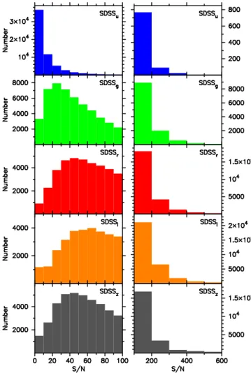
Since the exposure time is the same for all stars observed within a plate, the signal-to-noise ratio (S/N) of the acquired spectra varies significantly from target to target, which is mainly a reflection of their magnitude distribution. Because the number of available LAMOST spectra is huge, we decided to semiau-tomate the process of selection of high- and low-quality spec-tra using the information yielded by the LAMOST pipeline, namely, the values of S/N at the effective wavelengths of the Sloan DSS filters ugriz (Fukugita et al. 1996;Tucker et al. 2006) and the spectral type given either in the Harvard system or in a free, descriptive system of classification used in the LAMOST pipeline (e.g., carbon or flat). For targets classified by the LAM-OST pipeline as A, F, G, or K-type, we rejected spectra with S/N < 10 in the r filter. Spectra of targets classified to the other types were checked by eye to find and reject those that contain only noise. In Fig.1, we show histograms of S/N at the ugriz filters for the LAMOST spectra for which we derived the atmo-spheric parameters. In Table1, we give an overview of the an-alyzed LAMOST spectra. In total, the atmospheric parameters were derived from 61,753 LAMOST spectra, which correspond to 51 385 unique targets, including 30 213 stars that were ob-served by Kepler. For 8832 objects, more than one LAMOST spectrum was analyzed.
Fig. 1.Histograms of the S/N of the spectra from which we derived the
atmospheric parameters with the ROTFIT code measured at the effec-tive wavelengths of the Sloan DSS filters ugriz. The left and right panels show the S/N range [0, 100] with bin size 10 and the S/N range [100, 600] with bin size 100, respectively.
3. Data analysis
3.1. Radial velocity
The radial velocity was measured by means of the cross-correlation between the target spectrum and a template chosen among a list of 20 spectra of stars with different spectral types (Table2) taken from the Indo US library (Valdes et al. 2004). We chose stars with v sin i as low as possible to minimize the enlarge-ment of the cross-correlation function (CCF). However, given the low resolution of the LAMOST spectra (R ' 1800 with the slit width at 2/3 of the fiber size) and the coarse grid of spectral points, where the spacing corresponds to about 70 km s−1, only stars that are rotating faster than about 120 km s−1can have an appreciable effect on the CCF (see Sect.3.2).
The Indo-US spectra are suitable RV templates, since they are in the laboratory frame, i.e., the barycentric correction was already applied and the RV of the star subtracted. We only had to handle the continuum normalization.
Each LAMOST spectrum was split into eight spectral seg-ments centered at about 4000, 4500, 5000, 5500, 6200, 6700, 7900, and 8700 Å, and, for each segment, the CCF with each template listed in Table2 was computed. We therefore
devel-Table 1. Statistical overview of the analyzed LAMOST spectra that have been obtained before the end of the 2014 observation season for the Kepler FOV.
Field RA(2000) Dec(2000) Date # Spectra KO
LK01 19:03:39.26 +39:54:39.2 110 530 1 939 411 110 608 2 711 370 140 602 2 3386 1846 LK02a 19:36:37.98 +44:41:41.8 120 604 1 382 247 140 913 2 5439 3469 LK03b 19:24:09.92 +39:12:42.0 120 615 3 4614 3381 LK04c 19:37:08.86 +40:12:49.6 120 617 3 4206 2769 LK05 19:49:18.14 +41:34:56.8 131 005 2 3271 2247 140 522 1 1170 865 LK06 19:40:45.38 +48:30:45.1 130 522 1 1774 1317 130 914 1 2234 1530 LK07 19:21:02.82 +42:41:13.1 130 519 1 1778 1340 130 926 1 2324 1772 LK08d 19:59:20.42 +45:46:21.1 130 925 2 4330 1759 131 002 1 100 31 131 017 1 1674 660 131 025 1 2147 821 LK09 19:08:08.34 +44:02:10.9 131 004 1 2462 1702 LK10 19:23:14.83 +47:11:44.8 140 520 2 2041 1395 LK11 19:06:51.50 +48:55:31.8 140 918 1 2589 1649 LK12 18:50:31.04 +42:54:43.7 131 007 1 2111 1170 LK13 18:51:11.99 +46:44:17.5 140 502 1 1921 1075 140 529 2 3410 1841 LK14 19:23:23.79 +50:16:16.6 140 917 1 2588 1397 140 927 1 1814 974 140 929 1 2338 1158 Total 61 753 37 196 Unique 51 385 30 213 1× 42 553 24 303 2× 7569 5007 3× 1079 784 4× 117 81 +5× 67 38
Notes. The top lines give the specifications of the LK fields that have been observed. For each LK field, we give the right ascension (RA(2000)) and declination (DE(2000)) of the centrum, date of obser-vation (YYMMDD; Date), number of plates that were used to observe the LK field (#), number of spectra for which we derived the atmo-spheric parameters with the ROTFIT code (Spectra), and number of spectra that correspond to a target that was observed by the Kepler mis-sion (KO). The bottom lines give the summary of the observations of all LK fields together. We give the total number of spectra for which we derived the atmospheric parameters with the ROTFIT code (Total), number of different objects that were analyzed (Unique), and number of targets for which we obtained one (1×), two (2×), three (3×), four (4×), and at least five (+5×) sets of atmospheric parameters.(a) Includes the
cluster NGC 6811.(b) Includes the cluster NGC 6791.(c) Includes the
cluster NGC 6819.(d)Includes the cluster NGC 6866.
oped an ad hoc code in the IDL2environment. The best template was selected based on the height of the peak. To evaluate the centroid and full width at half maximum (FWHM) of the CCF peak, we fitted it with a Gaussian. For each spectral segment, the RV error, σi, was estimated by the fitting procedure curvefit
2 IDL (Interactive Data Language) is a registered trademark of Exelis
A&A 594, A39 (2016) Table 2. Templates adopted for the cross-correlation.
Name Sp. type Teffa v sin i (K) (km s−1) HD 47839 O7 Ve 40175 67b HD 180 163 B2 .5IV 18946 10c HD 17081 B7 IV 12678 25c HD 123 299 A0 III 10307 25d HD 34578 A5 II 8570 14d HD 25291 F0 II 7761 13e HD 33608 F5 V 6428 16.0f HD 88986 G0 V 5787 1.0f HD 115 617 G5 V 5598 1.1g HD 145 675 K0 V 5292 0.6h HD 32147 K3 V 4617 0.8i HD 88230 K8 V 3947 3.1h G 227-46 M3 V 3481 <2.8l HD 204 867 G0 Ib 5705 6.3m HD 107 950 G6 III 5176 6.6n HD 417 K0 III 4858 1.7n HD 29139 K5 III 3863 2.0n HD 168 720 M0 III 3789 . . . HD 123 657 M4 III 3235 . . . HD 126 327 M8 III 3088 . . .
References. (a) Wu et al. (2011); (b) Howarth (1997); (c) Abt et al.
(2002); (d) Royer et al. (2002); (e) Abt & Morrel (1995);
( f ) Nordström et al.(2004); (g) Queloz et al.(1998);(h) Fekel(1997);
(i) Saar & Osten (1997); (l) Delfosse et al. (1998); (m) Gray & Toner
(1987);(n)de Medeiros & Mayor(1999).
(Bevington 1969), taking the CCF noise into account, which was
evaluated far from the peak (|∆RV| > 4000 km s−1). The final RV for each star was obtained as the weighted mean of the values of all the analyzed spectral segments, using as weights wi = 1/σ2i, and applying a sigma clipping algorithm to reject outliers. The standard error of the weighted mean was adopted as the estimate of the RV uncertainty, σRV. The resulting RV and σRVvalues are given in columns 15 and 16 of TableA.3.
The RV errors are typically in the range 10–30 km s−1with an average value of about 20 km s−1. These errors are in line with what is expected on the basis of the LAMOST resolution and data sampling. In particular, less than 0.03% of the stars have an error σRV ≤ 10 km s−1, while 10 ≤ σRV < 20 km s−1 for 66% of the full sample, 20 ≤ σRV < 30 km s−1for 29% , 30 ≤ σRV< 40 km s−1for about 3.5%, and σRV≥ 40 km s−1for about 1.5% of the sample. The behavior of these errors as a function of SNRris shown in Fig.2. The median value ranges from about 18 km s−1to 27 km s−1as a function of S/N.
An empirical determination of the measurement uncer-tainty, however, can be performed by comparing repeated mea-surements of RV for the same star in different spectra (e.g.,
Yanny et al. 2009; Jackson et al. 2015). The distribution of the
RV differences is plotted in Fig. 3a. This distribution shows broad tails and it is best fitted by a double-exponential (Laplace) function (see, e.g., Norton 1984) rather than by a normal dis-tribution (Gaussian). The standard deviation of the Laplace fit is
√
2b = 16.6 km s−1, where b is the dispersion parameter of the Laplace function. Considering that this distribution is for RV differences of couples of measures, we must divide by √2 to ob-tain an estimate of the average error on each individual measure (e.g.,Jackson et al. 2015), which is b = 11.7 km s−1. This may
Fig. 2.Scatter plots with the errors of RV, Teff, log g, and [Fe/H] (from
top to bottom) as a function of the S/N in the r band. The following color coding is used: blue for 2011–2012, black for 2013, and red for 2014. The full green line, in each box, is the median value as a function of S/N.
suggest a slightly better RV precision than that indicated by the individual RV errors reported in TableA.3and plotted in Fig.2.
For 104 of the stars that we analyzed, we found RV values in the literature that come from high- or mid-resolution spectra. We discarded the stars known to be spectroscopic binaries (SB) and those with large pulsation amplitudes, for example, Mira-type variables, even if their RV variations are small compared to the typical LAMOST RV errors. To validate the RV deter-minations and to evaluate their external accuracy, we compared our measurements with those from the literature. The results are shown in Fig.4. The RV values and errors are also reported in TableA.1together with those from the literature for these stars. For most of these objects we have only one LAMOST spectrum, but for some of them we have from two to four different spec-tra with a total of 133 RV values. As it appears in Fig.4, our values of RV are consistent with the literature values within 3σ. There is only one star for which we found at least one discrepant RV value; this star is indicated with a filled circle enclosed in an open square in Fig.4. We considered an RV value as discrepant when |RVLAM − RVLit| ≥ 3
q (σLAM
RV ) 2+ (σLit
RV)
Fig. 3.Distributions of the differences of RV, Teff, log g, and [Fe/H] for the stars with repeated observations (histograms). In each box, the full line
is the double-exponential (Laplace) fit, while the dotted line is the Gaussian fit.
RV difference is larger than three times the quadratic sum of the errors. This object is KIC 7599132 (=HD 180757), which has been classified as a rotationally variable star byMcNamara et al.
(2012). We inserted this star in our ongoing campaign at the Catania Astrophysical Observatory aimed at a spectroscopic monitoring of newly discovered binary systems. As a very pre-liminary result, we can confirm its RV variations. The full results of this spectroscopic monitoring will be presented in a forthcom-ing paper.
This example shows that the LAMOST RVs are accurate enough to detect pulsating stars or single-lined spectroscopic bi-nary systems (SB1) with a large variation amplitude (∆RV > 50 km s−1when σ
RV≤ 20 km s−1) among the stars with multiple observations. To this purpose, for stars with multiple observa-tions, we calculated the reduced χ2and probability P(χ2) that the RV variations have a random occurrence (e.g.,Press et al. 1992). The values of P(χ2) are quoted in column 19 of TableA.3.
On average, the offset between the LAMOST and literature RVs is only+5 km s−1 and the rms scatter of our data around the bisector is '14 km s−1, which confirms the reliability of our RV measurements and their errors. In any case, if we take into account that some of these stars, especially those with only one LAMOST RV value, could indeed be undetected SBs, the dis-persion of 14 km s−1 can be considered an upper limit for the accuracy of our RV determinations.
The procedure for the measurement of RV was run inside the code for the determination of the atmospheric parameters (see Sect.3.2), since the RV was needed to align in wavelength the reference spectra with the observed one.
3.2. Projected rotation velocity and atmospheric parameters We estimated the projected rotation velocity, v sin i, and the at-mospheric parameters (APs), Teff, log g, and [Fe/H] with a ver-sion of the ROTFIT code (e.g.,Frasca et al. 2003,2006), which we adapted to the LAMOST spectra. We adopted, as templates, the low-resolution spectra of the Indo-US Library of Coudé Feed Stellar Spectra (Valdes et al. 2004) whose parameters were re-cently revised byWu et al.(2011). This library has the advan-tage of containing a large number of spectra of different stars, which sufficiently cover the space of the atmospheric parame-ters, even if the density of templates is not uniform and is rather low in the very metal poor regime. Although the small number of metal-poor templates is a limit for the determination of the APs, the use of spectra of real stars is beneficial for spectral sub-traction, as the synthetic spectra are more prone to problems in the cores of Hα and Ca
ii
-IRT lines (see, e.g.,Linsky et al. 1979;Montes et al. 1995).
The resolution of ≈1 Å and the sampling of 0.44 Å pixel−1 are both higher than the LAMOST resolution and sampling, and allow us to properly degrade the Indo-US spectra to match the
Fig. 4.Top panel: comparison between the RV measured on LAM-OST spectra (TableA.1) with literature values based mainly on high-resolution spectra (open circles). Filled circles refer to stars with mul-tiple LAMOST observations. The continuous line is the one-to-one re-lationship. The differences, shown in the bottom panel, show a mean value of '+5 km s−1 (dashed line) and a standard deviation of about
14 km s−1(dotted lines). Discrepant values are indicated with filled
cir-cles enclosed in squares in both panels.
LAMOST resolution and to resample them on the same length scale as the LAMOST spectra. Furthermore, the wave-length range covered by these spectra (from 3465 to 9470 Å) is larger than the wavelength range of the LAMOST spectra (from 3700 to 9000 Å), which allows us to exploit all the informa-tion contained in the LAMOST spectra for our analysis. We dis-carded those stars for which some parts of the spectrum were missing from the full library and kept 1150 templates.
In the first step, the reference spectra were aligned onto the target spectrum as a result of the radial velocity measured as de-scribed in Sect.3.1. In the second step, each template was broad-ened by the convolution with a rotational profile of increasing v sin i (in steps of 5 km s−1) until a minimum of the residuals was reached. This can provide us with an estimate of v sin i. However, given the low resolution of the LAMOST spectra, R ' 1800,
A&A 594, A39 (2016) which corresponds to about 170 km s−1, and the spectra
sam-pling of about 70 km s−1, this parameter is badly defined. We were only able to use it to unambiguously identify the very fast rotators in our sample. We ran Monte Carlo simulations with LAMOST spectra of a few stars, known to be slow rotators from the literature, with the aim of estimating the minimum v sin i that can be measured with our procedure. These spectra were arti-ficially broadened by convolution with a rotation profile of in-creasing v sin i (in steps of 30 km s−1) and a random noise was added, similar to Frasca et al.(2015). We found that the rota-tional broadening is unresolved up to 90 km s−1and we start to resolve it when v sin i ≥ 120 km s−1. We therefore can only trust v sin i values above 120 km s−1. For stars with a resulting v sin i value below 120 km s−1, the calculated value was replaced by <120 km s−1and flagged as an upper limit in TableA.3.
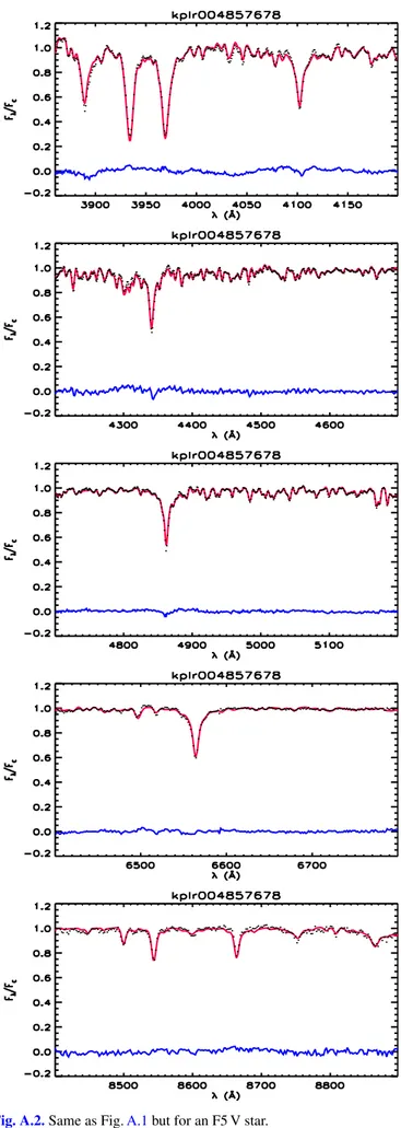
As for the RV, we split the spectrum into eight spectral seg-ments that were analyzed independently. The templates were then sorted in a decreasing order of the residuals, giving the highest score to the best-fitting template. The spectral type of the template with the highest total score, summing up the results of the individual spectral regions, was assigned to the target star. An example of the fit of an early A-type star, in five spectral seg-ments, is shown in Fig.A.1. Two other examples are shown in Figs.A.2andA.3for an F5 V and a K0 III star, respectively.
For each segment we derived values of Teff, log g, and [Fe/H] and their standard errors, which were based on the parameters of the ten best matching templates. The final APs were obtained as the weighted mean of those of the individual segments and are reported in Cols. 9, 11, and 13 of Table A.3, respectively. We adopted as uncertainties for Teff, log g, and [Fe/H] the standard errors of the weighted means to which the average uncertainties of the APs of the templates (±50 K, ±0.1 dex, ±0.1 dex, respec-tively) were added in quadrature. Scatter plots of APs errors as a function of the S/N in the r band are shown in Fig.2.
We also considered the stars with two or more spectra for the evaluation of the AP uncertainties, as we did for the RV. The distributions of Teff, log g, and [Fe/H] differences are indi-cated with the histograms in Figs.3b, c, and d, respectively. All these distributions are best fitted by a double-exponential func-tion whose dispersion parameter b indicates an average uncer-tainty of about 66 K or 1.3% for Teff, 0.046 dex for log g, and 0.055 dex for [Fe/H]. These values are all significantly smaller than the average errors (full lines in Fig. 2), which are likely slightly overestimated.
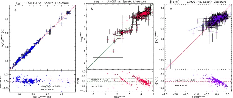
Both these evaluations of uncertainties are internal to the procedure and do not reveal the accuracy of the APs derived with ROTFIT and the templates’ grid of choice. To this aim we compared the parameters that were derived in the present work with those available for some stars from the literature. The lit-erature values were mainly derived from high-resolution opti-cal spectra and, in some cases, with asteroseismic techniques. The APs derived from LAMOST spectra, together with those found in the literature (468 stars with Teffdata, of which 352 and 350 also have log g and [Fe/H] values, respectively), are listed in TableA.2. The results of the comparison are shown in Fig.5.
We note the very good agreement between the Teff values with an average offset of only +30 K and an rms of 150 K in the temperature range 3000–7000 K (FGKM spectral types). As the errors of Teff determinations usually grow with the tempera-ture, we preferred to plot the logarithm of temperature in Fig.5, whose dispersion, σlog(Teff) = 0.4343σln(Teff) ' 0.4343σTeff/Teff, is a measure of the relative accuracy of temperature. This turns out to be σTeff/Teff ' 3.5% with no significant systematic offset with respect to the literature values.
The log g values display instead a larger scatter, which amounts to about 0.30 dex and a tendency for our values to clus-ter around 2.5 (the typical log g of the K stars in the red giant branch) and 4–4.5 (main-sequence stars). This is likely the result of the different density of templates as a function of log g that, at any given Teff, are more frequent at log g ' 4.5 and log g ' 2.5, giving rise to a possible bias toward MS or red-giant gravities in the average log g. We note that our analysis code derives a correct log g for several stars with literature values of log g that are intermediate between MS and giants or lower than 2.5. This comparison shows that the log g values are not very accurate, but we are still able to distinguish between luminosity classes I, III, and V, which, together with an accurate Teff determination unaffected by interstellar extinction, was one of the main aims of this analysis. Indeed, this is the requirement for performing a trustworthy spectral subtraction and flux calibration of the chro-mospheric EWs (see Sect. 3.4) because the surface continuum flux depends mainly on Teffand exhibits only a second-order de-pendence on log g that is properly considered with our gravity estimates (see AppendixC).
The [Fe/H] values are only in good agreement with the lit-erature values around the solar metallicity, i.e., between −0.3 and+0.2. We tend to overestimate [Fe/H] when it is lower than −0.3 and to underestimate it for values higher than +0.2. Al-though the data scatter could be due to the low resolution of the spectra, the systematic trend is likely an effect of the rel-ative scarcity of metal poor and super metal rich stars among our templates. Interestingly, the very low value of metallicity for KIC 9206432 ([Fe/H] = −2.23) has been correctly found by ROTFIT in the LAMOST spectrum, which indicates a negligi-ble contamination by metal richer templates. A linear fit to the values with [Fe/H]Lit > −1.5 (dashed line in Fig. 5c) gives a slope of m= 0.428 ± 0.029.
A large and very recent data set of APs for red gi-ants in the Kepler field is given in the APOKASC catalog
(Pinsonneault et al. 2014). They analyzed APOGEE near-IR
spectra, complemented with asteroseismic surface gravities. We found 787 stars in common. The comparison of the APs for these stars is shown in Fig.6. Even if the ranges of Teffand log g val-ues are smaller than those of Fig.5, these plots show the same general trends as in Fig.5. In particular, the agreement of Teff is rather good with an rms dispersion of 127 K and only two out-liers that we denoted with open squares.
The log g values display a systematic deviation from the one-to-one relation, which is similar to that shown by the giant stars in Fig.5 with the LAMOST gravities clustered around the av-erage value of red giants (∼2.5). This behavior is clearly shown by the differences plotted in the lower box. The outliers of the Teffplot show also discrepant log g values; these values are indi-cated with red dots enclosed in open squares in Fig.6b and the properties of these objects are described in AppendixB.
The plot of [Fe/H] comparison is very similar to that of Fig.5. In this case the systematic trend of the LAMOST versus APOKASC metallicity is even more evident and best fitted with a linear relation in the range of [Fe/H]APOKASC > −1.5, which roughly corresponds to [Fe/H]LAMOST > −1.0. We find a slope m= 0.464 ± 0.017, which is close to that of the fit of Fig.5. We thus propose a correction relation for the LAMOST metallicity, based on this linear fit, which can be expressed as
[Fe/H]corr= 2.16 · [Fe/H] + 0.17, (1)
applicable in the range [Fe/H] > −1.0.
Fig. 5.Comparison between the atmospheric parameters measured on LAMOST spectra with literature values. The continuous lines in the top panelsrepresent one-to-one relationships, as in Fig.4. The dash-dotted line in the [Fe/H] plot (panel c)) is a linear fit to the data with [Fe/H]Lit>
−1.5. The differences are shown in the bottom panels along with their average values and standard deviations.
Fig. 6.Comparison between the atmospheric parameters of red giants in the APOKASC catalog and in our database of LAMOST spectra. The meaning of symbols and lines is the same as in Fig.5. The open diamonds in the bottom box of panel c) refer to [Fe/H] values corrected according
to Eq. (1).
The LAMOST values of [Fe/H] corrected with the above equation are plotted in the bottom panel of Fig.6as green open diamonds. As shown in the figure, the trend has disappeared at the cost of a greater dispersion of the data. However, we prefer to report, in TableA.3, the [Fe/H] values as derived by our code without applying any correction to them, but these raw values should be corrected with Eq. (1) (or with purposely developed relations in their proper range of validity) before they are used.
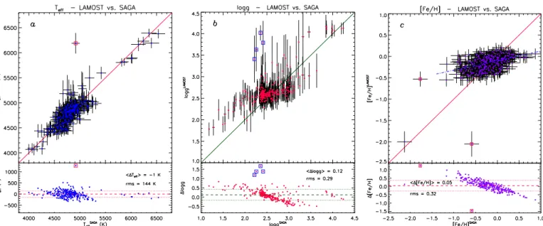
Another large set of atmospheric parameters for stars in the Kepler field is represented by the SAGA catalog
(Casagrande et al. 2014), which is based on asteroseismic data
and Strömgren photometry. Currently, this catalog contains pa-rameters for about 1000 objects, 287 of which have been
analyzed in the present paper. The results of the comparison of LAMOST and SAGA parameters are shown in Fig. 7, where symbols and lines have the same meaning as in Figs.5 and6. The comparison with SAGA data displays behaviors similar to those already found with the other data sets. Some outliers were also detected and indicated with open squares in Fig.7. These outliers are briefly discussed in AppendixB.
Similar to what we did for [Fe/H], we made an attempt to find a correction relation for log g. For this purpose we con-sidered all the stars with log g values in the literature (Fig.5b) from the APOKASC (Fig.6b) and the SAGA (Fig. 7b) cata-logs. These data are shown together, using different symbols, in Fig.8. As the log g values are basically grouped into two sepa-rate regions, we performed two different linear fits for log g < 3.3
A&A 594, A39 (2016)
Fig. 7.Comparison between the atmospheric parameters in the SAGA catalog and in our database of LAMOST spectra. The meaning of symbols and lines is the same as in Fig.5.
and log g ≥ 3.3, which are shown in Fig.8by the dash-dotted and dashed lines, respectively, and are given by the following equa-tions:
log gcorr= 2.01 · log g − 2.70 (log g < 3.3) (2) log gcorr= 1.88 · log g − 3.55 (log g ≥ 3.3).
This correction removes much of the nearly linear trends that appear in the bottom panel of Fig.8, although the scatter is en-hanced. As with [Fe/H], we report only the original values, with-out any correction, in TableA.3.
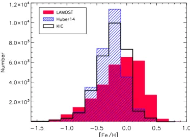
3.3. Statistical properties of the LAMOST-Kepler sample Figure9shows a comparison of the metallicity distributions of the LAMOST-Kepler targets derived in the present work (where [Fe/H] has been corrected according to Eq. (1)) with those from the KIC catalog and from the work ofHuber et al.(2014). For a meaningful comparison, we selected all the stars in common be-tween these three catalogs (30 104 stars). The different distribu-tions of LAMOST and KIC metallicities is apparent. The mean and median for the LAMOST data are −0.05 and+0.02 dex, re-spectively, while for the KIC data they are −0.17 and −0.13 dex, respectively. This result is in close agreement with the finding of
Dong et al.(2014), which strengthens the validity of the
correc-tion expressed by Eq. (1), at least in a statistical sense. The Huber et al. metallicities are distributed in a very similar way to that of the KIC catalog (mean= −0.19 dex; median = −0.16 dex). This is not surprising because the majority of these values are not spectroscopic and are mostly derived from the KIC photometry. Indeed, if we only consider the spectroscopic data inHuber et al.
(2014), we find a mean of −0.02 dex and a median of −0.01 dex, which are much closer to those of the LAMOST data.
The RV distribution for the full sample of LAMOST spectra is shown in Fig. 10, in which we also overplot the RV distri-butions for the subsamples in three different metallicity ranges. The distribution is far from symmetric and displays a tail to-ward negative radial velocities. The asymmetry of the distribu-tion is clearly enhanced with the decrease of metallicity, as ex-pected from the higher percentage of high-velocity stars among the metal poor stars.
Fig. 8.Comparison between our log g values and those from the litera-ture (blue dots), the APOKASC (red dots), and the SAGA (green aster-isks) catalogs. Linear fits to the data with log g < 3.3 and log g ≥ 3.3 are shown with the dash-dotted and dashed lines, respectively. The open diamonds in the bottom panel refer to values corrected according to Eq. (2).
As a further test on our results, we built the RV distribu-tion obtained with the SEGUE data (Yanny et al. 2009) in the Kepler field. We selected stars with coordinates in the range 275◦ ≤ RA ≤ 305◦ and 35.5◦ ≤ Dec ≤ 52.5◦. Because of the different selection criteria (mainly the limiting magnitude) for the Kepler-LAMOST and SEGUE surveys, only 13 stars are in common in the two samples. Nevertheless, the SEGUE sample
Fig. 9. [Fe/H] distribution (red filled histogram) for the
LAMOST-Keplersubsample of stars in common with theHuber et al.(2014) cat-alog (blue hatched histogram). The metallicities from the KIC catcat-alog are shown with the empty histogram.
Fig. 10.RV distribution for the full sample of spectra (empty histogram) and for the subsamples in specific metallicity ranges, as indicated in the legend. A bin size of 20 km s−1was used.
is composed of 3039 stars, which are spatially distributed as in Fig. 11a. Therefore it is statistically significant. As seen in Fig.11b, its RV distribution shows a shape that is very similar to that of LAMOST RVs. These data also display the larger contri-bution of stars with negative velocity at low metallicities.
3.4. Activity indicators and spectral peculiarities
Despite the rather low resolution, which prevents a detailed study of individual spectral lines, the LAMOST spectra are also very helpful to identify objects with spectral peculiarities such as emission lines ascribable, for example, to magnetic activity for late-type stars or to the circumstellar environment and winds in hot stars.
The most sensitive diagnostics of chromospheres in the range covered by the LAMOST spectra are the Ca
ii
H and K lines that lie, however, in a spectral region where the instrument efficiency is very low, compared to the red wavelengths. Moreover, the flux emitted by cool stars at the Caii
H and K wavelengths is very low36 38 40 42 44 46 48 50 52 279 282 285 288 291 294 297 300 DEC 2000 (deg) RA2000 (deg) a) 1 10 100 1000 -600 -400 -200 0 200 400 600 Number RV (km/s)
b) -0.3 ≤ [Fe/H]Full sample
-1.0 ≤ [Fe/H] < -0.3 [Fe/H] < -1.0
Fig. 11.Upper panel: spatial distribution of the SEGUE targets (dots) in the Kepler field. Lower panel: RV distribution for the SEGUE targets. A bin size of 20 km s−1was used.
and, with the exception of the brightest targets, is dominated by the noise in the LAMOST spectra.
We have therefore used the Balmer Hα line to identify late-type or early-late-type objects with emission, which can be produced by various physical mechanisms. We subtracted the Indo-US template that best matches the final APs from each LAMOST spectrum. This template has been aligned to the target RV and re-sampled on its spectral points. The residual Hα emission, EWres
Hα, was integrated over a wavelength interval of 35 Å around the line center (see Fig.12, upper panel). The stars with a residual Hα equivalent width EWHαres ≥ 1 Å were selected as emission-line candidates. A visual inspection of their spectra allowed us to re-ject several false positives, which are the result of (i) a mismatch in the line wings between target and template; (ii) a spurious emission inside the Hα integration range, which derives from a residual cosmic ray spike; and (iii) problems occurring in spectra with a very low signal. This selection criterion can be too strict for some stars, such as K and M dwarfs, with a filled-in pro-file or an intrinsically narrow Hα emission of moderate intensity that can be smeared by the low resolution to a signature with an EWHαres < 1 Å. For this reason we scrutinized all the spectra for which we found a Teff < 5000 K and a log g > 3.0 inte-grating the residual Hα profile over a smaller range (16 Å) and adopting 0.3 Å as the minimum EWres
Hαvalue for keeping a star as a candidate. This allowed us to select, after a visual inspec-tion of the results, addiinspec-tional stars that are likely to be active. As an example, we show in Fig.13the spectrum of KIC 4929016, which we classified as a K7V star (Teff = 4035 K). This star displays a weak Hα emission feature with an equivalent width of about 0.90 Å. This star has an RV (TableA.1) derived from the APOGEE survey of M dwarfs (Deshpande et al. 2013) and
A&A 594, A39 (2016)
Fig. 12.Upper panel: LAMOST spectrum of KIC 4637336 (black dot-ted line), a late G-type star with the Hα totally filled in by emission. The inactive template is overplotted with a thin red line. The difference be-tween target and template spectrum, plotted in the bottom of the panel (blue line), shows only a residual Hα emission (hatched area). The in-tegration range for the residual equivalent width, EWres
Hαis indicated by
the two vertical lines and the two regions used for the evaluation of the continuum setting error are also denoted. Lower panel: the spectral re-gion around the Ca
ii
infrared triplet (IRT) is shown with the same line styles as for Hα. The residual chromospheric emission in the cores of the Caii
IRT lines is outlined by the hatched areas.is known to display a strong and nearly continuous flare activ-ity from the Kepler light curves analyzed by Walkowicz et al.
(2011).
We selected a total of 577 spectra of 547 stars displaying Hα in emission or filled in by a minimum amount as defined above. The values of EWHα, along with their errors, are quoted in TableA.4. We also report whether the line is observed as a pure emission feature and whether the measure is uncertain as a result of the low S/N or other possible spectral issues.
For these stars we also investigated the behavior of the Ca
ii
IRT by subtracting the same inactive template used for the Hα (see lower panels of Figs.12and13). For late-type active stars, the emission, which fills the cores of the Caii
lines, originates from a chromosphere. The equivalent widths of the residual Caii
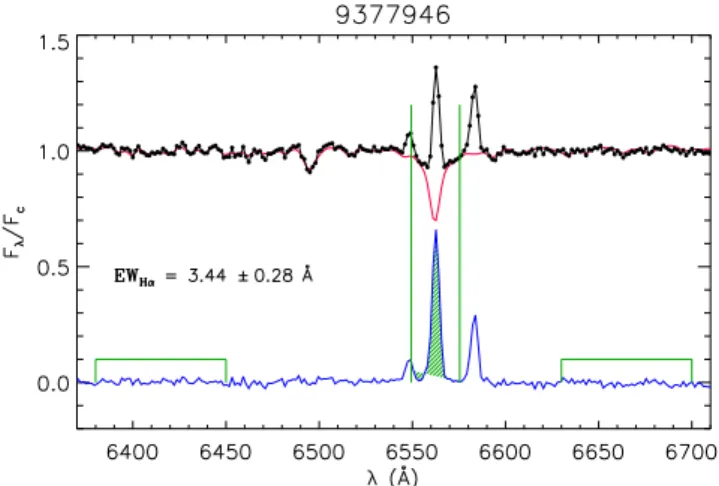
IRT emission lines, EW8498res , EW8542res , and EW8662res , are also given in TableA.4.In some cases we saw two emission lines at the two sides of the Hα emission that are, without any doubt, the forbidden lines [N
ii
] at λ 6548 and λ 6584 Å. This pattern is best observed in the residual spectrum (see Fig.14). These lines are normally observed in ionization nebulae. We think that these emissionFig. 13.Hα emission in the LAMOST spectrum of KIC 4929016. Lines and symbols are as in Fig.12.
Fig. 14.Example of a star where the Hα line is dominated by nebu-lar sky emission superimposed on the stelnebu-lar spectrum. The forbidden nitrogen lines at the two sides of Hα appear both in the original and subtracted spectrum.
features can be the result of nebular emission that has not been fully removed by the sky subtraction. Indeed, the intensity of nebular emission was observed to be strongly variable over small spatial scales, from arcminutes down to a few arcseconds (e.g.,
O’Dell et al. 2003;Hillenbrand et al. 2013), and the sky fibers
in the LAMOST field of view. We also flagged these stars in TableA.4.
4. Chromospheric activity
For stars cooler than about 6500 K, for which the sub-photospheric convective envelopes are deep enough to permit an efficient dynamo action, the Hα and Ca
ii
cores are suitable diagnostics of magnetic activity. The best indicators of chromo-spheric activity, rather than the EW of a chromochromo-spheric line, are the surface line flux, F, and the ratio between the line luminosity and bolometric luminosity, R0, which are calculated, for the Hα, asFHα = F6563EWHαres (3)
R0Hα = LHα/Lbol= FHα/(σTe4ff), (4) where F6563is the continuum surface flux at the Hα center, which has been evaluated from the NextGen synthetic low-resolution spectra (Hauschildt et al. 1999) at the stellar temperature and surface gravity of the target. The line fluxes in the three Ca
ii
IRT lines were calculated with similar relations, where the con-tinuum flux at the center of each line was also evaluated from the NextGen spectra. For each line, the flux error includes both the EWerror and uncertainty in the continuum flux at the line center, which is obtained by propagating the Teffand log g errors.The Hα fluxes and R0
Hαof our targets are plotted as a func-tion of the effective temperature in Fig. 15, along with the boundary between the accreting objects (mostly located above this line) and the chromospherically active stars, as defined by
Frasca et al. (2015). Different symbols are used for stars with
solid measures of EWHαres (blue dots) and those where the detec-tion of the Hα core filling is less secure (green asterisks) either because of a low S/N, problems in the spectrum, or the pres-ence of nebular emission lines. This figure clearly shows a dif-ferent lower level of fluxes and R0for stars with T
eff< 5000 K and Teff> 5000 K, which is the result of the two thresholds adopted for selecting active stars in the two Teffdomains.
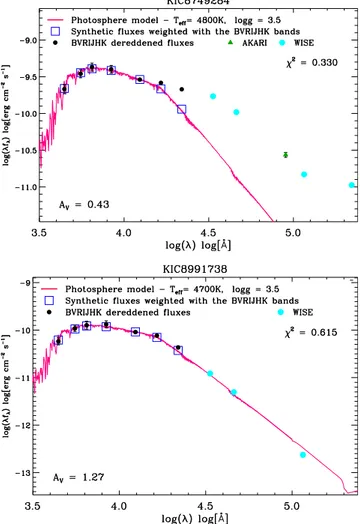
We point out that only one star is located in the region occupied by accreting stars. This object, KIC 8749284, is de-noted with “1” in Fig. 15b. It was classified by ROTFIT as K1 V and it is the star with the highest value of EWHαres (13 Å). In the only spectrum acquired by LAMOST there is no clear evidence of lithium absorption, which is normally observed in young accreting objects. Alternatively, this object could be an active close binary (SB2 or SB1) composed of main-sequence or evolved stars. Nevertheless, a young age is supported by the infrared (IR) colors, which place KIC 8749284 in the domain of Class II objects in the 2MASS and WISE color-color dia-grams (e.g., Koenig et al. 2012). Besides, the spectral energy distribution (SED) clearly shows an IR excess starting from the Hband, which is compatible with an evolved circumstellar disk of a Class II source (see Fig.16). The fit of the SED has been performed as inFrasca et al.(2015) from the B to J band, adopt-ing the effective temperature found by ROTFIT for the photo-spheric model and letting the interstellar extinction AV free to vary. This star displays rotational modulation in the Kepler pho-tometry with a period of about 3.2 days (Debosscher et al. 2011). Follow-up spectroscopic observations with a higher resolution would help to unveil its nature.
The star labeled “2”, which lies close to the dividing line in Fig.15, is KIC 8991738. Its SED does not show any IR excess (Fig.16). Although it is included in the KIC, it has never been observed by Kepler. The target “3”, KIC 4644922 (=V677 Lyr),
has an anomalously high level of chromospheric activity for such a hot star. It was previously classified as a semiregular variable (e.g., Pigulski et al. 2009). Indeed, according toGorlova et al.
(2012), KIC 4644922 is a candidate post-AGB star surrounded by a dusty disk for which the Hα emission originates in the cir-cumstellar environment. The spectra of star “4” (KIC 8722673) and “5” (KIC 9377946) show the clear pattern of nebular emis-sion with the two forbidden nitrogen lines at the two sides of Hα (see Fig.14for KIC 9377946). We think that, for these two stars, the strong Hα flux does not have a chromospheric origin but is mostly the result of sky line emission that overlaps the stellar spectrum.
In Fig. 17 we compare the Hα and Ca
ii
chromospheric fluxes. The latter, FCaII−IRT, is the sum of the flux in each line of the triplet. We limited our analysis to the GKM stars (Teff < 6000 K) to minimize the contamination by sources for which the emission does not have a chromospheric origin. How-ever, this subsample (442 stars) is a large portion of the sam-ple of active objects that were selected as described in Sect.3.4. The two fluxes are clearly correlated, as indicated by the Spear-man’s rank correlation coefficient ρ = 0.62 with a significance of σ = 4.35 × 10⁻²⁴(Press et al. 1992). A least-squares regression yields the following relation:log FHα= −1.85 + 1.25 · log FCaII−IRT, (5) where we took the bisector of the two least-squares regressions (X on Y and Y on X). A power law with an exponent larger than 1 for this flux–flux relationship is in agreement with previ-ous results (see, e.g.,Martínez-Arnáiz et al. 2011, and reference therein).
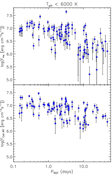
For about 200 stars we found the rotation periods in the literature (Debosscher et al. 2011; Nielsen et al. 2013;
Reinhold et al. 2013;McQuillan et al. 2013,2014;Mazeh et al.
2015). We found that, besides the scatter, the Hα flux increases with decreasing rotation period, Prot, as shown in Fig. 18. The correlation with Prot is an expected result, based on the αΩ dynamo mechanism, and it is widely documented in the literature for several diagnostics of chromospheric and coro-nal activity (e.g.,Frasca & Catalano 1994; Montes et al. 1995;
Pizzolato et al. 2003; Cardini & Cassatella 2007; Reiners et al.
2015, and references therein). The Spearman rank correlation analysis, which is limited to the stars with solid measures of Hα emission (blue dots in Fig. 18) and Teff < 6000 K, yields a correlation coefficient ρ = −0.59 with a significance of σ = 2.5 × 10⁻¹¹, which means a highly significant correlation be-tween FHαand Prot. A similar behavior, albeit with a lower de-gree of correlation (ρ = −0.18; σ = 0.07), is displayed by the Ca
ii
-IRT flux. We think that the low resolution of the spectra, which gives rise to rather large flux errors, and the heterogeneous sample, which includes stars with very different properties, are mainly responsible for the large data scatter. The latter prevents us, for example, from clearly distinguishing the saturated and unsaturated activity regimes.5. Summary
We are carrying out a large spectroscopic survey of the stars in the Kepler field using the LAMOST spectrograph. In this pa-per we present the results of the analysis of the spectra obtained during the first round of observations (2011–2014), which are mainly based on the code ROTFIT.
We selected spectra with Hα emission and chromospheri-cally active stars by means of the spectral subtraction of inactive
A&A 594, A39 (2016)
Fig. 15.Left panel: Hα flux vs. Teff. Right panel: R0
Hαvs. Teff. In both panels the candidates with a questionable emission are denoted with green
asterisks. The dashed straight line is the boundary between chromospheric emission (below it) and accretion as derived byFrasca et al.(2015).
Fig. 16.Spectral energy distribution of the two stars cooler than 5500 K with the highest R0
Hαvalues. Note the IR excess for KIC 8749284.
templates chosen in a large grid of real-star spectra. Because of the low resolution and rather low S/N for most of the surveyed stars, we set an EW threshold that minimizes the contamination
Fig. 17.Flux–flux relationship between Hα and Ca
ii
IRT. The meaning of the symbols is as in Fig.15. The dashed line is the least-squares regression.with false positive detections. For cool stars (Teff < 6000 K) we also calculated the Hα and Ca
ii
-IRT fluxes, which are important proxies of chromospheric activity.In total, we analyzed 61 753 spectra of 51 385 stars perform-ing an MK spectral classification, evaluatperform-ing their atmospheric parameters (Teff, log g, and [Fe/H]) and deriving their radial ve-locity (RV). Our code also allows us to measure the projected rotation velocity (v sin i) that, because of the low resolution of the LAMOST spectra, is possible only for fast-rotating stars (v sin i > 120 km s−1).
Fig. 18.Hα and Ca
ii
-IRT flux vs. Prot.To check the data quality, we searched in the literature for values of the parameters derived from high- or intermediate-resolution spectra. The comparison of the LAMOST Teff val-ues with those from the literature (468 stars in the range 3000– 20 000 K) shows a very good agreement and indicates an accu-racy of about 3.5%. The comparison with literature values for log g (352 stars) displays a larger scatter and the tendency of LAMOST values to cluster around the average log g of main-sequence stars (∼4.5) and red giants (∼2.5). Similarly, for [Fe/H] we found a systematic trend, which is best observed when our data are compared with those from the APOKASC catalog (787 stars in common). We proposed a correction relation for the metallicities derived with ROTFIT from the LAMOST spectra, which is based on these comparisons. These effects are likely the result of both the low resolution and the uneven distributions of the spectral templates in the space of parameters. Anyway, the accuracy of the log g and [Fe/H] measurements is sufficient to perform a discrete luminosity classification and to sort the stars in bins of metallicity. This allows us to get a safe flux calibration of the lines EWs.
Our RV measurements agree with literature data within 14 km s−1, which we consider the external accuracy. Despite the rather low LAMOST resolution, we could identify interesting and peculiar objects, such as stars with variable RV (SB or pul-sating star candidates), ultrafast rotators, and stars in particular evolutionary stages.
Our data display a different metallicity distribution compared to that obtained from the Sloan photometry, with a median value that is higher by about 0.15 dex. This result is in agreement with previous findings based on smaller data samples, supporting the validity of the correction relation for [Fe/H] that we proposed.
The RV distribution is asymmetric and shows an excess of stars with negative RVs which is larger at low metallicities. This results is in agreement with the data of the SEGUE survey in the Keplerfield.
Based on the Hα and Ca
ii
-IRT fluxes, we have found 442 chromospherically active stars, one of which is a likely accreting object, as indicated by the strong and broad Hα emission and by the relevant infrared excess. The availability of precise rotation periods from the Kepler photometry has allowed us to study the dependency of these chromospheric fluxes on the rotation rate for a very large sample of field stars. We found that both the Hα and Caii
-IRT fluxes are correlated with the rotation period, with the former diagnostic showing the largest decrease with the increasing Prot.Acknowledgements. The authors are grateful to the anonymous referee for very useful suggestions. Guoshoujing Telescope (the Large Sky Area Multi-Object Fibre Spectroscopic Telescope LAMOST) is a National Major Scientific Project built by the Chinese Academy of Sciences. Funding for the project has been pro-vided by the National Development and Reform Commission. lamost is operated and managed by the National Astronomical Observatories, Chinese Academy of Sciences. We thank Katia Biazzo and Gijs Mulders for helpful discussions and suggestions. Support from the Italian Ministero dell’Istruzione, Univer-sità e Ricerca(MIUR) is also acknowledged. J.M.- ˙Z. acknowledges the fund-ing received from the European Community’s Seventh Framework Programme (FP7/2007–2013) under grant agreement No. 269194 and grant number NCN 2014/13/B/ST9/00902. J.N.F. and A.N.R. acknowledge the support of the Joint Fund of Astronomy of National Natural Science Foundation of China (NSFC) and Chinese Academy of Sciences through the Grant U1231202, and the Na-tional Basic Research Program of China (973 Program 2014CB845700 and 2013CB834900). Y.W. acknowledges the National Science Foundation of China (NSFC) under grant 11403056. This research made use of SIMBAD and VIZIER databases, operated at the CDS, Strasbourg, France. This publication makes use of data products from the Two Micron All Sky Survey, which is a joint project of the University of Massachusetts and the Infrared Processing and Analysis Center/California Institute of Technology, funded by the National Aeronautics and Space Administration and the National Science Foundation. This publica-tion makes use of data products from the Wide-field Infrared Survey Explorer, which is a joint project of the University of California, Los Angeles, and the Jet Propulsion Laboratory/California Institute of Technology, funded by the Na-tional Aeronautics and Space Administration.
References
Abt, H. A., & Morrel, N. I. 1995,ApJS, 99, 135
Abt, H. A., Levato, H., & Grosso, M. 2002,ApJ, 573, 359
Allende Prieto C., et al. 2008,Astron. Nachr., 329, 1018
Balona, L. A., Pigulski, A., De Cat, P., et al. 2011,MNRAS, 413, 2043
Barbier-Brossat, M., Petit, M., & Figon, P. 1994,A&AS, 108, 603
Batalha, N. M., Rowe, J. F., Bryson, S. T., et al. 2013,ApJS, 204, 24
Bevington, P. 1969, in Data Reduction and Error Analysis for the Physical Sciences (New York: Mc Graw-Hill), 237
Brown, T. M., Latham, D. W., Everett, M. E., & Esquerdo, G. A. 2011,AJ, 144, 24
Bruntt, H., Frandsen, S., & Thygesen, A. O. 2011,A&A, 528, A121
Bruntt, H., Basu, S., Smalley, B., et al. 2012,MNRAS, 423, 122
Buchhave, L. A., Latham, D. W., Johansen, A., et al. 2012,Nature, 486, 375
Cardini, D., & Cassatella, A. 2007,ApJ, 666, 393
Casagrande, L., Schönrich, R., Asplund, M., et al. 2011,A&A, 530, A138
Casagrande, L., Silva Aguirre, V., Stello, D., et al. 2014,ApJ, 787, 110
Casagrande, L., Silva Aguirre, V., Schlesinger, K. J., et al. 2016,MNRAS, 455, 987
Catanzaro, G., Frasca, A., Molenda- ˙Zakowicz, J., & Marilli, E. 2010,A&A, 517, A3
Catanzaro, G., Ripepi, V., Bernabei, S., et al. 2011,MNRAS, 411, 1167
Debosscher, J., Blomme, J., Aerts, C., & De Ridder, J. 2011,A&A, 529, A89
De Cat, P., Fu, J. N., Ren, A. B., et al. 2015,ApJS, 220, 19(Paper I) Delfosse, X., Forveille, T., Perrier, C., & Mayor, M. 1998,A&A, 331, 581
A&A 594, A39 (2016)
Deshpande, R., Blake, C. H., Bender, C. F., et al. 2013,AJ, 146, 156
de Medeiros, J. R., & Mayor, M. 1999,A&AS, 139, 433
Dong, S., Zheng, Z., Zhu, Z., et al. 2014,ApJ, 789, L3
Famaey, B., Jorissen, A., Luri, X., et al. 2005,A&A, 430, 165
Fehrenbach, C., Duflot, M., Mannone, C., Burnage, R., & Genty, V. 1997,
A&AS, 124, 255
Fekel, F. C. 1997,PASP, 109, 514
Frasca, A., & Catalano, S. 1994,A&A, 284, 883
Frasca, A., Alcalá, J. M., Covino, E., et al. 2003,A&A, 405, 149
Frasca, A., Guillout, P., Marilli, E., et al. 2006,A&A, 454, 301
Frasca, A., Fröhlich, H.-E., Bonanno, A., et al. 2011,A&A, 523, A81
Frasca, A., Biazzo, K., Lanzafame, A. C., et al. 2015,A&A, 575, A4
Frinchaboy, P. M., & Majewski, S. R. 2008,AJ, 136, 118
Fröhlich, H.-E., Frasca, A., Catanzaro, G., et al. 2011,A&A, 543, A146
Fukugita, M., Ichikawa, T., Gunn, J. E., et al. 1996,AJ, 111, 1748
Gilmore, G., et al. 2012,Messenger, 147, 25
Gontcharov, G. A. 2006,Astron. Lett., 32, 759
Gorlova, N., Van Winckel, H., & Jorissen, A. 2012,Balt. Astron., 21, 165
Gray, D. F., & Toner, C. G. 1987,ApJ, 322, 360
Gray, R. O., Corbally, C. J., De Cat, P., et al. 2016,AJ, 151, 13
Grenier, S., Baylac, M.-O., Rolland, L., et al. 1999,A&AS, 137, 451
Hauck, B., & Mermilliod, M. 1998,A&AS, 129, 431
Hauschildt, P. H., Allard, F., & Baron, E. 1999,ApJ, 512, 377
Hillenbrand, L. A., Hoffer, A. S., & Herczeg, G. J. 2013,AJ, 146, 85
Howarth, I. D., Siebert, K. W., Hussain, G. A. J., & Prinja, R. K. 1997,MNRAS, 284, 265
Hubble E. 1942,Science, 95, 212
Huber, D., Chaplin, W. J., Christensen-Dalsgaard, J., et al. 2013,ApJ, 767, 127
Huber, D., Silva Aguirre, V., Matthews, J. M., et al. 2014,ApJS, 211, 2
Jackson, R. J., Jeffries, R. D., Lewis, J., et al. 2015,A&A, 580, A75
Kepler, J. 1609, Astronomia nova
Kharchenko, N. V., Scholz, R.-D., Piskunov, A. E., Röser, S., & Schilbach, E. 2007, Astron. Nachr., 328, 889
Koenig, X. P., Leisawitz, D. T., Benford, D. J., et al. 2012,ApJ, 744, 130
Lehmann, H., Tkachenko, A., Semaan, T., et al. 2011,A&A, 526, A124
Linsky, J. R., Hunten, D. M., Sowell, R., Glackin, D. L., & Kelch, W. L. 1979,
ApJS, 41, 481
Luo A.-L., Zhang, H.-T., Zhao, Y.-H., et al. 2012,RA&A, 12, 1243
Luo, A.-L., Zhao, Y.-H., Zhao, G., et al. 2015,RA&A, 15, 1095
Mann, A. W., Gaidos, E., Lépine, S., & Hilton, E. J. 2012,ApJ, 753, 90
Marcy, G. W., Isaacson, H., Howard, A. W., et al. 2014,ApJS, 210, 20
Martínez-Arnáiz, R., López-Santiago, J., Crespo-Chacón, I., & Montes, D.,
MNRAS, 414, 2629
Mazeh, T., Perets, H. B., McQuillan, A., & Goldstein, E. S. 2015,ApJ, 801, 3
McNamara, B. J., Jackiewicz, J., & McKeever, J. 2012,AJ, 143, 101
McQuillan, A., Mazeh, T., & Aigrain, S. 2013,ApJ, 775, L11
McQuillan, A., Mazeh, T., & Aigrain, S. 2014,ApJS, 211, 24
Mermilliod, J. C., Mayor, M., & Udry S. 2008,A&A, 485, 303
Meszaros, Sz., Holtzman, J., Garcia Perez, A. E., et al. 2013,AJ, 146, 133
Molenda- ˙Zakowicz, J., Frasca, A., Latham, D. W., & Jerzykiewicz, M. 2007,
Acta Astron., 57, 301
Molenda- ˙Zakowicz, J., Frasca, A., & Latham, D. W. 2008,Acta Astron., 58, 419
Molenda- ˙Zakowicz, J., Latham, D. W., Catanzaro, G., Frasca, A., & Quinn, S. N. 2011,MNRAS, 412, 1210
Molenda- ˙Zakowicz, J., Sousa, S. G., Frasca, A., et al. 2013,MNRAS, 434, 1422
Molenda- ˙Zakowicz, J., Brogaard, K., Niemczura, E., et al. 2014,MNRAS, 445, 2446
Montes, D., Fernández-Figueroa, M. J., De Castro, E., & Cornide, M. 1995,
A&A, 294, 165
Nidever, D. L., Marcy, G. W., Butler, R. P., Fischer, D. A., & Vogt, S. S. 2002,
ApJS, 141, 503
Nielsen, M. B., Schunker, H., Gizon, L., & Ball, W. H. 2015,A&A, 582, A10
Niemczura, E., Murphy, S. J., Smalley, B., et al. 2015,MNRAS, 450, 2764
Nordström, B., Mayor, M., Andersen, J., et al. 2004,A&A, 418, 989
Norton, R. M. 1984, The American Statistician (American Statistical Association), 38, 135
O’Dell, C. R., Peimbert, M., & Peimbert, A. 2003,AJ, 125, 2590
Pakhomov, Yu. V., Antipova, L. I., Boyarchuk, A. A., Zhao, G., & Liang, Ya. 2009,Astron. Rep., 53, 685
Petigura, E. A., Marcy, G. W., & Howard, A. W. 2013,ApJ, 770, 69
Pigulski, A., Pojma´nski, G., Pilecki, B., & Szczygieł, D. M. 2009,Acta Astron., 59, 33
Pinsonneault, M. H., Elsworth, Y., Epstein, C., et al. 2014,ApJS, 215,
Pizzolato, N., Maggio, A., Micela, G., Sciortino, S., & Ventura, P. 2003,A&A, 397, 147
Pojma´nski, G. 1997,Acta Astron., 47, 467
Press, W. H., Teukolsky, S. A., Vetterling, W. T., & Flannery, B. P. 1992, Numerical Recipes in Fortran 2nd edn. (Cambridge: Cambridge Univ. Press) Queloz, D., Allain, S., Mermilliod, J.-C., Bouvier, J., & Mayor, M. 1998,A&A,
335, 183
Reiners, A., Schüssler, M., & Passegger, V. M. 2014,ApJ, 794, 144
Reinhold, T., Reiners, A., & Basri, G. 2013,A&A, 560, A4
Ren, A. B., Fu, J. N., De Cat, P., et al. 2016, ApJS, submitted
Royer, F., Grenier, S., Baylac, M.-O., Gómez, A. E., & Zorec, J. 2002,A&A, 393, 897
Saar, S. H., & Osten, R. A. 1997,MNRAS, 284, 803
Shapley, H., & Curtis, H. D. 1921,Bulletin of the National Research Council, 2, 171
Steinmetz, M., et al. 2006,AJ, 132, 1645
Thygesen, A. O., Frandsen, S., Bruntt, H., et al. 2012,A&A, 543, A160
Tkachenko, A., Lehmann, H., Smalley, B., Debosscher, J., & Aerts, C. 2012,
MNRAS, 422, 2960
Torres, G., Fischer, D. A., Sozzetti, A., et al. 2012,ApJ, 757, 161
Tucker, D. L., Kent, S., Richmond, M. W., et al. 2006,Astron. Nachr., 327, 821
Udalski, A., Szymanski, M., Kału˙zny, J., Kubiak, M., & Mateo, M. 1992,Acta Astron., 42, 253
Uytterhoeven, K., Briquet, M., Bruntt, H., et al. 2010,Astron. Nachr., 331, 993
Uytterhoeven, K., Moya, A., Grigahcène, et al. 2011,A&A, 534, A125
Valdes, F., Gupta, R., Rose, J. A., Singh, H. P., & Bell, D. J. 2004.ApJS, 152, 251
Walkowicz, L. M., Basri, G., Batalha, N., et al. 2011,AJ, 141, 50
Wang, S.-G., Su, D.-Q., Chu, Y.-Q., Cui, X., & Wang, Y.-N. 1996,Apl. Opt., 35, 5155
Wang, J., Fischer, D. A., Barclay, T., et al. 2013,ApJ, 776, 10
Wilson, R. E. 1953, in General Catalogue of Stellar Radial Velocities (Carnegie Inst. Washington D.C. Publ.), 601
Wu, Y., Singh, H. P., Prugniel, P., Gupta, R., & Koleva, M. 2011,A&A, 525, A71
Wu, Y., Du, B., Luo, A., Zhao, Y., & Yuan, H. 2014, in Statistical Challenges in 21st Century Cosmology, Proc. IAU Symp., 306, 340
Xing, X., Zhai, C., Du, H., et al. 1998,Proc. SPIE, 3352, 839
Yanny, B., Rockosi, C., Newberg, H. J., et al. 2009,AJ, 137, 4377
York D. G., et al. 2000,AJ, 120, 1579
Zhao, G., Zhao, Y.-H., Chu, Y.-Q., Jing, Y.-P., & Deng, L.-C. 2012,RA&A, 12, 723
Appendix A: Additional data
Fig. A.1.Example of the continuum-normalized LAMOST spectrum of an early A-type star in five spectral regions (dots). The best template found by ROTFIT is overplotted with a thin red line. The difference between the two spectra is shown in the bottom of each panel with a blue full line.
A&A 594, A39 (2016)
Table A.1. Stars with radial velocity in the literature.
KIC Name HJD RVLAM σLAMRV RVLit σLitRV Reference
(−2 400 000) (km s−1) (km s−1) 1 726 211 TYC 2667-624-1 56 094 .21294 −129.1 17.3 −145.80 ... T12 1 861 900 HD 181 655 56 094 .25369 −19.0 21.0 2.03 0.09 N02 1 873 543 2MASS J19302029+3723437 56 094 .29879 12.3 21.6 23.06 0.35 D13 2 425 631 TYC 3120-1300-1 56 811 .25084 32.9 17.8 19.10 ... T12 2 837 475 HD 179 260 55 721 .30256 −5.6 29.4 −13.00 0.70 N04 3 430 868 HD 179 306 55 721 .30252 22.6 25.2 5.40 ... T12 3 563 082 HD 186 506 56 096 .24488 −14.5 18.3 −22.10 0.30 G06 3 657 793 HD 185 562 56 096 .27008 −15.7 19.8 -0.44 0.42 F05 3 748 585 BD+38 3601 56 096 .26934 −0.5 18.3 −5.80 ... T12 3 748 691 TYC 3134-261-1 56 096 .26934 2.9 20.0 −0.10 ... T12 3 860 139 TYC 3135-696-1 56 096 .26924 −2.4 18.3 −25.20 ... T12 3 955 590 TYC 3134-31-1 56 096 .24501 −49.6 18.0 −57.20 ... T12 4 070 746 TYC 3135-326-1 56 096 .26919 9.5 19.3 −1.60 ... T12 4 161 741 HIP 95 913 56 096 .26927 −21.6 20.4 −22.84 0.16 M08 4 177 025 TYC 3136-647-1 56 096 .24579 −87.0 16.8 −123.10 ... T12 4 242 575 HD 176 845 55 721 .30254 −19.2 19.2 −32.30 2.80 N04 4 283 484 HD 225 666 56 096 .27009 −23.5 17.4 −44.80 ... T12 4 283 484 HD 225 666 56 570 .97671 −52.1 16.3 −44.80 ... T12 4 283 484 HD 225 666 56 800 .32810 −18.0 19.1 −44.80 ... T12 4 352 924 HD 179 733 56 094 .22092 −5.1 24.8 −18.50 2.50 G06 4 352 924 HD 179 733 55 721 .28765 10.6 23.6 −18.50 2.50 G06 4 484 238 HIP 97 236 56 096 .27008 −6.9 19.0 −14.78 0.34 M11 4 574 610 HIP 96 775 56 096 .24482 −31.5 24.0 −44.52 0.45 M11 4 581 434 HD 186 997 56 096 .24574 −0.3 28.6 −4.30 6.20 C10 4 581 434 HD 186 997 56 570 .97672 −13.5 25.4 −4.30 6.20 C10 4 581 434 HD 186 997 56 800 .32808 39.2 38.6 −4.30 6.20 C10 4 659 706 TYC 3139-1785-1 56 096 .26918 −10.0 16.4 −21.80 ... T12 4 914 923 BD+39 3706 56 094 .22083 −51.0 19.8 −25.46 1.01 M07 4 929 016 2MASS J19330692+4005066 56 096 .26915 −11.5 15.6 −20.10 0.07 D13 5 113 061 TYC 3140-2350-1 56 096 .26908 24.6 18.0 −4.30 ... T12 5 113 910 2MASS J19421943+4016074 56 096 .30212 18.5 16.3 −12.40 ... T12 5 206 997 HIP 97 337 56 096 .27060 −56.6 27.2 −70.50 0.49 M07 5 206 997 HIP 97 337 56 570 .97674 −78.9 16.2 −70.50 0.49 M07 5 206 997 HIP 97 337 56 800 .32802 −59.9 20.4 −70.50 0.49 M07 5 284 127 TYC 3139-1918-1 56 570 .97656 −73.1 16.8 −73.00 ... T12 5 442 047 HIP 94 952 56 094 .25340 −54.5 21.1 −53.92 0.18 M08 5 511 423 2MASS J18523459+4046480 56 572 .95996 −109.7 18.0 −87.30 ... T12 5 524 720 2MASS J19160889+4044237 56 094 .21277 −46.5 23.1 −32.80 ... T12 5 524 720 2MASS J19160889+4044237 56 562 .00867 −38.9 15.9 −32.80 ... T12 5 612 549 TYC 3125-195-1 56 094 .25339 −11.0 20.0 −3.50 ... T12 5 612 549 TYC 3125-195-1 56 562 .00870 −12.3 15.3 −3.50 ... T12 5 701 829 BD+40 3689 56 432 .26132 1.3 16.0 −20.50 ... T12 5 709 564 TYC 3139-1534-1 56 094 .21261 −79.4 21.2 −104.90 ... T12 5 786 771 HD 182 192 56 432 .26132 21.7 23.7 −21.70 12.10 C10 5 792 581 TYC 3138-169-1 56 094 .21263 −2.5 20.4 5.20 ... T12 5 859 492 TYC 3124-1301-1 55 721 .28761 −37.1 27.1 −59.40 ... T12 6 289 468 BD+41 3389 56 096 .25166 3.3 34.7 0.51 0.42 Tk12 6 289 468 BD+41 3389 56 562 .01362 −13.4 22.0 0.51 0.42 Tk12 6 579 998 TYC 3126-920-1 56 572 .95987 −58.4 15.2 −43.40 ... T12 6 680 734 TYC 3129-1020-1 56 432 .26135 26.9 16.3 12.60 ... T12 6 696 436 BD+41 3390 56 096 .24467 −19.8 22.8 −13.90 ... T12
Notes. B94 =Barbier-Brossat et al. (1994); C10 =Catanzaro et al. (2010); D13 =Deshpande et al. (2013); F05= Famaey (2005); F08 =
Frinchaboy (2008); F11 = Frasca et al. (2011); F12 = Fröhlich et al. (2012); F97 =Fehrenbach et al. (1997); G06 =Gontcharov (2006); G99=Grenier et. al.(1999); K07=Kharchenko et al.(2007); M07=Molenda- ˙Zakowicz et al.(2007); M08=Molenda- ˙Zakowicz et al.(2008); M11=Molenda- ˙Zakowicz et al.(2011); M14=Molenda- ˙Zakowicz et al.(2014); Me08=Mermilliod et al.(2008); N02=Nidever et al.(2002); N04=Nordström et al.(2004); P09=Pakhomov et al.(2009); T12=Thygesen et al.(2012); Tk12=Tkachenko et al.(2012); W53=Wilson
![Fig. 2. Scatter plots with the errors of RV, T eff , log g, and [Fe/H] (from top to bottom) as a function of the S/N in the r band](https://thumb-eu.123doks.com/thumbv2/123dokorg/8094954.124743/5.892.461.828.112.718/fig-scatter-plots-errors-rv-eff-function-band.webp)
![Fig. 3. Distributions of the differences of RV, T e ff , log g, and [Fe/H] for the stars with repeated observations (histograms)](https://thumb-eu.123doks.com/thumbv2/123dokorg/8094954.124743/6.892.70.837.115.263/fig-distributions-differences-rv-stars-repeated-observations-histograms.webp)