Relationships between running economy and mechanics in middle-distance runners

ALMA MATER STUDIORUM

UNIVERSITA’ DI BOLOGNA

Dottorato di Ricerca in

Discipline delle Attività Motorie e Sportive

XX ciclo

Sede amministrativa: Università di Bologna

Coordinatore: Prof. Salvatore Squatrito

Relationships between running economy and

mechanics in middle-distance runners

Tesi di Dottorato in

Metodi e Didattiche delle Attività Sportive (M-EDF/02)

Presentata da: Relatore:

ABSTRACT

Running economy (RE), i.e. the oxygen consumption at a given submaximal speed, is an important determinant of endurance running performance. So far, investigators have widely attempted to individuate the factors affecting RE in competitive athletes, focusing mainly on the relationships between RE and running biomechanics. However, the current results are inconsistent and a clear mechanical profile of an economic runner has not been yet established.

The present work aimed to better understand how the running technique influences RE in sub-elite middle-distance runners by investigating the biomechanical parameters acting on RE and the underlying mechanisms. Special emphasis was given to accounting for intra-individual variability in RE at different speeds and to assessing track running rather than treadmill running.

In Study One, a factor analysis was used to reduce the 30 considered mechanical parameters to few global descriptors of the running mechanics. Then, a biomechanical comparison between economic and non economic runners and a multiple regression analysis (with RE as criterion variable and mechanical indices as independent variables) were performed. It was found that a better RE was associated to higher knee and ankle flexion in the support phase, and that the combination of seven individuated mechanical measures explains ∼72% of the variability in RE.

In Study Two, a mathematical model predicting RE a priori from the rate of force production, originally developed and used in the field of comparative biology, was adapted and tested in competitive athletes. The model showed a very good fit (R2=0.86).

In conclusion, the results of this dissertation suggest that the very complex interrelationships among the mechanical parameters affecting RE may be successfully dealt with through multivariate statistical analyses and the application of theoretical mathematical models. Thanks to these results, coaches are provided with useful tools to assess the biomechanical profile of their athletes. Thus, individual weaknesses in the running technique may be identified and removed, with the ultimate goal to improve RE.

TABLE

OF

CONTENTS

2.1 RELATIONSHIP BETWEEN RUNNING ECONOMY AND PERFORMANCE……….………. 4

2.2 BIOMECHANICAL FACTORS AFFECTING RUNNING ECONOMY………. 6

2.2.1 KINEMATICS ...………..… 6

2.2.2 KINETICS ……… 8

2.2.3 ANTHROPOMETRY………...………….. 9

2.2.4 FLEXIBILITY………..………... 10

3. MATERIALS AND METHODS……….………... 12

3.1 SUBJECTS………..… 12

3.2 EXPERIMENTAL APPARATUS……… 13

3.2.1 THE COSMED K4B2 GAS ANALYSER………. 13

3.2.2 THE OPTOJUMP……… 14

3.2.3 THE SIMI MOTION SYSTEM………. 15

3.3.1 THE CONTINUOUS INCREMENTAL TEST………… 17

3.3.2 THE MULTISTAGE TEST……… 18

3.3.2.1 METABOLIC MEASURES……… 20

3.3.2.2 BIOMECHANICAL PARAMETERS………… 21

4. STUDY 1 – A STATISTICAL APPROACH TO THE INVESTIGATION OF THE RUNNING MECHANICS / ECONOMY RELATIONSHIP…………..……….… 26

4.1 INTRODUCTION……….. 26

4.2 STATISTICAL ANALYSES……….… 28

4.3 RESULTS………..……….. 28

4.3.1 FACTOR ANALYSIS………. 30

4.3.2 MECHANICAL DIFFERENCES BETWEEN ECONOMICAL AND NON-ECONOMICAL RUNNERS….. 32

4.3.3 MULTIPLE REGRESSION……….. 36

4.4 DISCUSSION………. 39

5. STUDY 2 – A MATHEMATICAL MODEL PREDICTING RUNNING ECONOMY FROM BIOMECHANICAL PARAMETERS..……..… 42

5.1 INTRODUCTION……….. 42

5.2 MODEL DERIVATION……….…………..….. 43

5.2.3 ESTIMATION OF THE FORCE TO SWING THE

LIMB….……… 47

5.2.4 THE COMPLETE MODEL………..… 48

5.3 RESULTS………...….... 50

5.3.1 TESTING OF PARTIAL COMPONENTS ……… 50

5.3.2 TESTING OF THE COMPLETE MODEL ………….. 52

5.4 DISCUSSION………... 53

6. GENERAL CONCLUSIONS…..……… 56

LIST OF FIGURES

3.1 The Cosmed K4b2 gas analyser………... 13

3.2 The Optojump system with multiple bars……… 14

3.3 The SIMI Motion Software……….…… 16

3.4 Determination of VO2max……….… 18

3.5 Determination of running economy from the multistage test………. 20

3.6 Conventions used for the angles………. 24

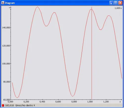
3.7 Example of a goniogram of the knee angle……….24

4.1 Oxygen uptake vs. running speed relationship for the ten runners…….… 32

4.2 Energy cost of running vs. running speed relationship for the ten runners……….…… 33

4.3 Predicted (through the multiple regression model) vs. observed VO2..….. 37

5.1 Estimated vertical and horizontal components of the ground reaction force……….……… 43

5.2 Determination of the limb angle at toe off ……….. 45

5.3 Mean vertical rate of force production (mFVERTrate) vs. RE .……….…... 50

5.4. Mean vertical + horizontal rate of force production (mF(HORIZ+VERT)rate)vs. RE……….………51

LIST OF TABLES

3.1 Characteristics of the experimental sample……….………12 3.2 Individual running speeds in the four stages of the multistage test………….19 4.1 Factor analysis……….…………30 4.2 Differences for kinematics among three RE groups……..……….………….34 4.3 Coefficients of independent variables in the multiple regression model ...….38

1.GENERAL INTRODUCTION

In competitive endurance running, the performance has been traditionally related to the maximum oxygen uptake (VO2max) (Costill 1967, Saltin 1967, Costill

1973, Hagan 1981, Boileau 1982, Brandon 1987). However, a large amount of studies has shown that running economy (RE), defined as the aerobic demand for a given submaximal speed (Morgan 1989a), is also a very important determinant of endurance ability, discriminating well the performance among athletes with similar VO2max (Bransford 1977, Conley 1980, Daniels 1985, Krahenbuhl 1989, Morgan

1989b, Di Prampero 1993).

Given the influence of RE on the performance in middle- and long-distance running competitions, applied scientists turned great efforts to discover which are the factors that mainly affect RE. In this research field, a large body of investigations was driven by the intuitive link between running technique and economy, i.e. by the logical reasoning that performing mechanical patterns without non-productive movements and applying forces of appropriate magnitude in the right directions with precise timing will result in less total work, less physiological strain and then improved performance (Anderson 1996). Therefore, several authors attempted to relate RE to biomechanical parameters as gait patterns (Cavanagh 1982, Williams 1987a, Williams 1987b), angular kinematics (Williams 1986, Williams 1987a, Anderson 1994, Lake 1996, Kyrolainen 2001), and ground reaction forces (Williams 1987a, Heise 2001).

Despite several researches have been carried out on this topic, only moderate relationships have been found and inconsistencies have appeared among studies,

while a clear biomechanical profile of an economic runner has not yet been established, as acknowledged in review articles (Morgan 1992, Anderson 1996, Saunders 2004a) and recently confirmed in a conference paper (Williams, 2007). The main reason of the lacking of definitive conclusions may be the extraordinary complexity of the interrelationships between the mechanical parameters determining running economy. As pointed in a review article by Anderson (1996), the mechanical factors related to RE do not act independently and weaknesses in a characteristic may be counterbalanced by some other element in the overall running mechanics. Then, the RE exhibited by an athlete reflects the integrate composite of a variety of physiological and mechanical characteristics, which is unique to that individual. These peculiarities may make very difficult to show any actual relationship between RE and single mechanical parameters. In further investigations, multivariate statistical techniques are to be used for a better understanding of the interactions among mechanical parameters and their overall influences on RE.

Another possible drawback of past studies is that most of them have considered just one or at best two submaximal running speeds when relating RE to mechanical parameters. This methodological choice may have been dictated by the assumption that the energy cost of running, i.e. the metabolic demand per unit of travelled distance, is invariant across speed in the same subject (Di Prampero 1993). However, empirical evidences and experimental data (Daniels 1992, Peroni Ranchet 2006) allow to affirm that this assumption is not true in all the athletes. Therefore it is opportune, when relating biomechanics and RE, to include into the analysis several different submaximal speeds. In this way, the intraindividual variability at different speeds may be taken into account.

In the first part of the present work (Study One), the relationships between RE and selected mechanical measures were analysed in sub-elite middle-distance runners taking into account the aforementioned concerns to past investigations. Multivariate statistics was used to individuate, discrete groups of parameters (factors) describing global elements of the running technique, to be related to RE. Four submaximal speeds, individually determined (corresponding to 60, 70, 80 and 90% of individual maximal aerobic velocity) were considered to account for intra-individual variability at different speeds. Furthermore, the evidence that athletes adapt individually and unpredictably their outdoor running technique to the treadmill (Nigg 1995) discouraged the use of the treadmill for this work, and the analysis was performed on outdoor running, with the use of a portable gas analyser.

The second part of this thesis was devoted to an alternative approach to the problem of relating running mechanics and economy, i.e. the use of a mathematical model predicting a priori the energy cost of running from some mechanical descriptors of the running gait. Despite this approach appears very promising to deal with the complex relationships between RE and running mechanics, it has not been considered so far in the field of sports science. Indeed, it was used in the comparative biology to investigate the influence of morphological characteristics on the energy cost of locomotion across different species (Kram 1990, Roberts 1998a, Roberts 1998b, Pontzer 2005, Pontzer 2007).

To address the effectiveness of such approach to understand the influence of running technique on RE in competitive athletes, a mathematical model predicting RE from the rate of muscular force production, was developed (adapted from Pontzer

2.LITERATURE REVIEW

2.1 Relationship between running economy and performance

The relationship between RE and performance has been widely documented in the last decades. An early research (Pollock 1977) comparing elite vs. good distance runners showed that the elite runners had a better RE than their weaker counterparts. The difference was exalted when expressing VO2submax as a percentage of VO2max,

with the elite runners consuming a lower percentage of their VO2max. Few years

later, Conley (1980) assessed RE in 12 elite distance runners of similar level, showing that RE was a good predictor of the performance in a 10 km race, being highly correlated (r ranging from 0.79 to 0.83) with the race time. A more recent study (Weston 2000) compared the RE and performance of Kenyan and Caucasian distance runners. Despite their 13% lower VO2max, Kenyans had similar 10 km race time

compared to Caucasians thanks to their 5% better RE. The Kenyan runners also completed the 10 km race at a higher percentage of their VO2max but with similar

blood lactate concentration levels than the Caucasian runners.

The interrelationships among running performance, VO2max, and RE among

trained subjects with similar VO2max have been examined in a cross-sectional work

by Morgan (1989b). In that study, RE was more related to 10 km race time than VO2max (r=0.64 vs. –0.45). However, the velocity at VO2max (vVO2max), predicted

combining the relative contributions of VO2max and RE, showed the highest

correlation with performance (r=-0.87).

Longitudinal studies supported the role of an optimal RE for a high level endurance performance. Conley (1981) monitored a top level runner weekly during

18 weeks of training. In this period, the athlete increased his VO2max from 70.2

ml·min-1·kg-1 to 76.1 ml·min-1·kg-1. In the same period his RE at 295 m·min-1 improved from 58.7 ml·min-1·kg-1 to 53.5 ml·min-1·kg-1. The same author (Conley 1984) reported similar data on a stronger athlete, the American mile record holder Steve Scott, who was tested before and after a 6-month training period. The athlete improved his VO2max to from 74.4 ml·min-1·kg-1 to77.2 ml·min-1·kg-1. During the

same period, his RE at a running speed of 268 m·min-1decreased to 45.3 ml·min-1·kg-1 from the initial (off season) value of 48.5 ml·min-1·kg-1. The combined improvement of VO2max and RE led to the reduction of the relative intensity of running from 65 to

58% of VO2max (Conley 1984).

Studies of groups with longitudinal designs have been also carried out. Daniels (1978) assessed young boys (10 to 18 years old), engaged in middle and long distance running training for 2 to 5 years. They did not changed their VO2max but

improved their performances thanks to an improved RE. Similar findings have been reported by Krahenbuhl (1989), who have analysed untrained boys (10 years old at the beginning) over a 7-year period. His results showed that despite the unchanged VO2max, the 9-minute run distance performance increased by 29% associated with a

13% reduction in the energy cost of submaximal running. Seasonal variations in RE and distance running performance have also been shown in elite adult runners (Svedenhag 1985). Those athletes undertook alternating sessions of slow distance, uphill and interval training over a 22-month period, showing significant reductions in RE at 15 and 20 km·h-1 associated to faster 5000m run times.

2.2 Biomechanical factors affecting running economy

2.2.1 Kinematics

Endurance running implies the conversion of muscular forces into complex movement patterns, involving all the major joints. An intuitive link exists between running technique and economy, since performing mechanical patterns without non-productive movements and applying forces of appropriate magnitude in the right directions with precise timing will result in the lesser energy consumption at a given running speed (Anderson 1996). Therefore, several investigators attempted to explain the inter-individual variations in RE through differences among runners in the biomechanical patterns of their running style.

The first descriptor of running style that has been related to the energy requirement of running has been stride length. Several studies (Hogberg 1952, Knuttgen 1961, Cavanagh 1982, Powers 1982, Kaneko 1987) have shown that runners self select the optimal stride length for a given speed, and RE tends to increase curvilinearly as stride length is altered (lengthened or shortened). Cavanagh (1982) stated that there is little need to dictate stride length for well trained athletes since they tend to display near optimal stride lengths. He suggested two mechanisms to explain this phenomenon. Firstly, runners naturally acquire an optimal stride length and stride rate over time, based on perceived exertion. Secondly, runners may adapt physiologically through repeated training at a particular stride length/stride frequency combination for a given running speed (Cavanagh 1982).

Several other discrete kinematic variables have been related to running economy. An early study of Cavanagh (1977) indicated that economic elite runners

had less vertical oscillation and were more symmetrical compared to less economic athletes. In a study carried out on elite male distance runners, Williams (1986) found that better RE was associated with a more extended lower leg at foot strike, a greater maximal plantarflexion velocity, and a greater horizontal heel velocity at foot strike. The same author (Williams 1987a) compared 3 groups of runners divided according to their RE at 3.6 m·s-1 (low, medium and high VO2) and found that better RE was

associated with higher shank angle with the vertical at the foot strike, less plantarflexion at toe-off and more flexed knee in the mid-support. The lesser amplitude of arm movements was also associated to better economy (Williams 1987a, Anderson 1994). A more recent research (Kyrolainen 2001) has related RE to several three-dimensional kinematic and kinetic parameters and EMG activity at different speeds. None of the considered kinematical indices (angular displacements between the ankle, knee and hip joints, joint angular velocities) was, taken alone, a good predictor of RE.

Although significant differences and trends have been observed between economic and non economic runners in some kinematical parameters, the relationships appear weak and inconsistent among studies. This is due to the complex interrelationships amongst the multitude of discrete mechanical descriptors of the running technique that globally influence RE. Therefore, definitive conclusions can not be traced on the basis of present data, and further studies using proper statistical analysis to deal with multiple variables are required.

2.2.2 Kinetics

A wide body of studies have related descriptors of ground reaction forces (GRF) to RE. Williams (1987) found that more economical runners showed significantly lower first peaks in the vertical component of the GRF and tended to have smaller horizontal and vertical peak forces. Basing on these results, they suggested that differences in the kinematics, especially before the foot strike, may affect the muscular demand and thus RE. Heise (2001) investigated the support requirements during foot contact of trained male runners. Higher total and net vertical impulse were shown in the less economical athletes, indicating wasteful vertical motion. The combined influence of vertical GRF and the time course of the force application explained 38% of the inter-individual variability in RE. However, other GRF characteristics such as medial-lateral or horizontal moments were not significantly correlated with RE. Kyrolainen (2001) found that the rate of force production increased with increasing running speed and that the horizontal (braking) component of the GRF was related to RE. They suggested that increasing the pre-landing and braking activity of the leg hamstrings muscles might prevent unnecessary yielding of the runner during the braking phase, with an enhancement of the musculo-tendon stiffness, and a resulting improvement in RE.

In summary, relationships between RE and GRF characteristics have been repeatedly shown, although the inherent mechanisms needs to be more clearly understood.

Insights to analyse the inter-individual variations in RE in competitive athletes come from the field of comparative biology. Kram (1990) investigated the aerobic demand of locomotion in a several animal species. He presented an inverse

relationship between RE and contact time, indicating that the energy cost of running is determined by the cost of supporting the animal’s mass and time course of generating force (Kram 1990). Subsequent studies confirmed that the requirement to support the body mass, expressed by vertical GRF, is the major metabolic cost of running (Farley 1992, Chang 1999). However, experiments applying impending and assisting horizontal forces demonstrated that also the horizontal component of GRF significantly affects the metabolic cost of running (Cooke 1991, Chang 1999). Finally, recent studies carried out on running animals and humans have clearly shown that the muscular force required to swing the limb also contribute to a significant amount to the energy expenditure (Marsh 2004, Modica 2005).

2.2.3 Anthropometry

Anthropometric characteristics such as limb dimensions and proportions have been addressed as potential influences on RE. Assuming that leg length contributes to angular inertia and the metabolic cost on moving the legs during running (Anderson 1996), it should be an important factor in determining RE. However, Williams (1987) found no differences in leg length between economic and non economic male distance runners. As for kinematic parameters, it is very unlike that a single anthropometric index may discriminate among different levels of RE, since RE is complexly affected by a multitude of interacting factors, and the effect of a single factor may be hidden by the others.

In contrast, there are some evidences that leg mass and leg mass distribution may influence RE. Studies in which the leg angular inertia has been altered with

increases RE by ∼1% (Catlin 1979, Martin 1985, Jones 1986). Myers (1985) studied 4 athletes trained to run with additional weight on the trunk, upper thigh, upper shank, and ankle. All limb loadings resulted in greater increases in cost of running than when the same mass was carried at the waist, with cost increasing as position of loads became more distal. Another research involving ankle and wrist loading (Clearmont 1988) revealed that RE was lowest for the unloaded condition, followed by ankle loading only, wrist loading only, and both wrist and angle loading. This research stream led to state that for a given body mass and a given speed, smaller and more proximally distributed limb mass results in lower kinetic energy required to accelerate and decelerate the limbs and thus lower cost of running.

2.2.4 Flexibility

Several studies contend that flexibility affect RE (Godges 1989, Gleam 1990, Craib 1996). Godges (1989) showed in athletic college students that RE improved with improved hip flexion and extension. This finding reflected the empirical belief that improved flexibility is desirable for increasing RE and may be explained by an enhanced neuromuscular balance due to the high flexibility, eliciting lower VO2submax. Contrarily, Gleam (1990) found that untrained subjects who exhibited

the lowest flexibility were the most economical. This was explained by inflexibility in the transverse and frontal planes of the trunk and hip regions of the body that stabilizes the pelvis at the foot strike. This may have the effect of reducing both excessive range of motion and metabolically expensive stabilising muscular activity (Gleam 1990). Craib et al. (1996) examined the relationship between RE and selected trunk and lower limb flexibility tests in trained male distance runners. Inflexibility in

the hip and calf was associated with better RE by minimising the need for muscle stabilising activity and increasing the storage of elastic energy. Another study (Jones 2002) found that lower limb and trunk flexibility was negatively related to RE in elite male distance runners. The author interpreted his results stating that improved RE may reflect greater stability of the pelvis, a reduced requirement for additional muscular activity at foot strike, and a greater storage and return of elastic energy due to inflexibility of the lower body (Jones 2002). Kyrolainen (2001) found that stiffer muscles around the ankle and knee joints in the braking phase of running increased force expression in the push-off phase. Therefore, stiffer and more inflexible muscles in the legs and lower trunk could enhance RE via increased energy from elastic storage and return. According to the review of Saunders (2004) the findings of these research taken together suggest that there is an optimal level of flexibility whereby RE can benefit, although a certain degree of muscle stiffness is also required to maximise elastic energy storage and return in the trunk and legs.

3.MATERIALS AND METHODS

3.1 Subjects

Ten well trained middle-distance runners volunteered to participate. Their characteristics are shown in Table 3.1.

Subject Age _(ys) Height _(cm)

Body mass (kg) VO2max (ml·min-1·kg -1₎ Training volume

(km·week-1₎ Personal best

1 25.45 175 65 72.32 80 4.14 (1500m) 2 29.57 186 76 60.03 55 4.22 (1500m) 3 26.03 171 61 65.36 90 15.23 (5000m) 4 27.42 172 66 63.5 75 16.13 (5000m) 5 23.45 173 59 69.27 80 14.44 (5000m) 6 24.87 181 72 71.33 100 15.32 (5000m) 7 28.44 171 63 74.7 100 3.58 (1500m) 8 27.94 182 60 70.52 95 16.23 (5000m) 9 24.63 174 72 72.43 70 4.24 (1500m) 10 20.37 174 58 68.56 90 15.10 (5000m) Mean (± SD) ± 2.57 25.82 175.9 ± 4.9 ±5.8 66.2 68.60 ±4.32 ± 13.6 83.5

TABLE 3.1. Characteristics of the experimental sample

All the athletes regularly participate to track and field competitions at regional and national level, therefore they represented a sample of the Italian sub-elite middle-distance runners population. The runners were healthy and free of injuries at the time of participation. They were recommended to refrain from any strenuous training for at least 3 days before each testing session.

3.2 Experimental apparatus

3.2.1 The Cosmed K4b

gas analyser

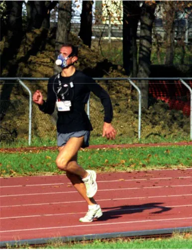
The K4b2 (Cosmed, Rome, Italy) is a portable telemetric device designed to collect and analyse expired air samples in a field context. The apparatus is attached to the athletes’ chest by means of special belts (Fig. 3.1).

FIGURE 3.1. The Cosmed K4b2 gas analyser

The gas analyser allows to collect several metabolic parameters, as oxygen uptake, carbon dioxide production, ventilation and all derived indices. Heart rate may also be registered and integrated with metabolic measures when the athlete wears a

common transmitting belt. The accuracy and test-retest reliability of the Cosmed K4b2 system have been previously shown (Duffield 2004).

3.2.2 The Optojump

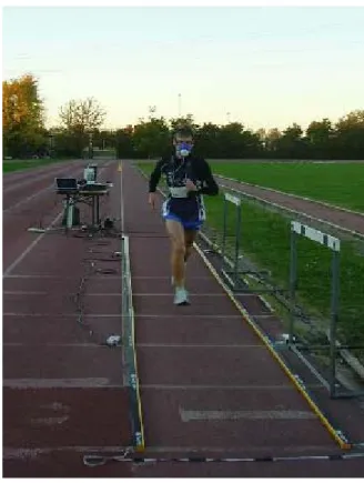
The Optojump (Microgate, Bolzano, Italy) is an infrared optical system allowing to measure contact and flight times during running, with an accuracy of 10-3 s. It is constituted by two parallel instrumented bars (100x3x4 cm), one containing the control and reception unit and the other the transmission unit. In the present work ten bars were connected together to increase to 10m the length of the path used for measurements, displaced on the first line of an athletic track (Fig. 3.2).

Thus, 5 to 8 consecutive foot strikes were available for each transit between the bars. The Optojump with multiple bars allows to obtain also the stride length, with a precision of 3 cm. In this study, data from Optojump were downloaded to a personal computer and processed through the interface software Optojump 3.01.

3.2.3 The SIMI motion analysis system

SIMI Motion (SIMI Reality Motion Systems, Unterschleissheim, Germany) is a 2D/3D video-based motion analysis software, especially suitable to study sportive actions in the field (Fig. 3.3). In fact, the movement is digitised offline on one ore more video clips captured from different angles with common digital cameras, needing no markers to be applied on the athlete’s body. The resulting pixel coordinates are then scaled and converted to real-world coordinates (i.e. measured in meters), allowing to obtain all the desired kinematic parameters (e.g. distances, angles or angular velocities).

3.3 Procedures

The subjects performed two incremental running tests on separate sessions. The first was a continuous test to determine maximal oxygen uptake and maximal aerobic velocity. The second was a multi-stage test to determine running economy, in which also biomechanical parameters were collected. Test protocols are described in detail in the next subsections.

Both the tests were carried out on a 400-m outdoor track, with stable meteorological conditions (sunny weather with no wind, ambient temperature: 16 – 21 °C). Reference cones were positioned every 50m along the track and the subjects followed an acoustic signal to maintain the prescribed pace. Prior to the test, subjects were familiarized with the procedure and instructed to adjust softly their speed when necessary, avoiding any abrupt acceleration or deceleration. The correspondence between the prescribed and the actual pace was checked by an operator carefully observing that the subject was in proximity to the cone at the right moment.

3.3.1 The continuous incremental test

Each subject completed a continuous incremental running test to exhaustion in which maximal oxygen uptake (VO2max) and the velocity where VO2max was

achieved, i.e. the maximal aerobic velocity (MAV), were determined. Initial speed was set at 12 km·h-1 and increased of 1 km·h-1 every lap (400m) until test termination. VO2 was continuously measured with the Cosmed K4b2 gas analyser. The VO2

associated to the stage in which VO2 max occurred was considered as the subject’s

MAV.

FIGURE 3.4. Determination of VO2max

Individual VO2max values are displayed in Table 3.1, while Table 3.2 (see

next paragraph) shows the MAVs.

3.3.2 The multistage test

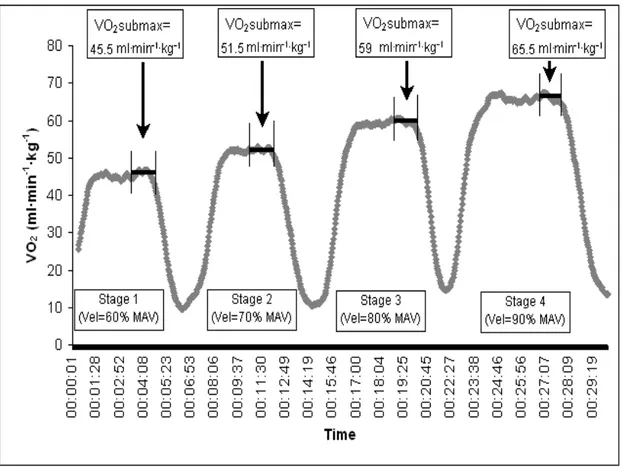
A 4 x 4-min multistage test with 4 min recovery between stages was performed to determine running economy and the energy cost of running. VO2 was

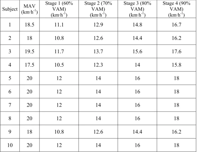
speeds of the four stages were individually established for each athlete, being equal respectively to 60, 70, 80, and 90% of the MAV. Table 3.2 displays the speeds used in the multistage test for the ten subjects.

Subject MAV (km·h-1) Stage 1 (60% VAM) (km·h-1₎ Stage 2 (70% VAM) (km·h-1₎ Stage 3 (80% VAM) (km·h-1₎ Stage 4 (90% VAM) (km·h-1₎ 1 18.5 11.1 12.9 14.8 16.7 2 18 10.8 12.6 14.4 16.2 3 19.5 11.7 13.7 15.6 17.6 4 17.5 10.5 12.3 14 15.8 5 20 12 14 16 18 6 20 12 14 16 18 7 20 12 14 16 18 8 20 12 14 16 18 9 18 10.8 12.6 14.4 16.2 10 20 12 14 16 18

TABLE 3.2. Individual running speeds in the four stages of the multistage test

Subjects covered 2 to 4 laps for each stage. At the end of each lap, the actual speed was checked through the data obtained with the Optojump system (see 3.2.2), with the formula speed = step length / (contact time + flight time). For each stage, the passage with the minor difference between the prescribed and actual velocity was selected and used for the subsequent analyses, with the largest accepted discrepancy

3.3.2.1 Metabolic measures

Running economy (RE), was obtained separately for each stage by averaging VO2 values of the last minute of that stage. An example of this procedure is provided

with a graphical explanation in Fig. 3.5.

FIGURE 3.5. Determination of running economy from the multistage test

The energy cost of running (Cr) is defined as the energy required above resting

to transport the subject’s body over one unit of distance (Di Prampero 1993). According to Lacour (1990), Cr (in ml·kg-1·m-1) was calculated for each subject at

each given velocity as Cr = (VO2-0.083) x v-1, where VO2 is expressed in ml·kg-1·s-1

value corresponding to the y-intercept of the VO2/v relationship established by

Medbo (1988) in young male adults.

The reliability of RE in elite distance runners obtained with a method similar to that used here have been previously verified (Saunders, 2004b)

3.3.2.2 Biomechanical parameters

During the multistage test, subjects were filmed in lateral view at 50 frames/s with a 3-megapixel camera (Dcr-Hc1000E, Sony, Japan), at every lap when they passed between the 10-m bars of the Optojump just before the arrival line of the track. The camera was positioned 8 m away from the first line of the track, framing a calibrated area about 12m long. Films were then downloaded to a PC and arranged to be digitised with the SIMI motion software for the subsequent 2D motion analysis.

For each frame, the following points were digitised on the subject’s image: • Head (tragus)

• Right and left hip (greater trochanter) • Right and left knee (lateral condyle) • Right and left ankle (lateral malleolus) • Right and left foot (base of the first phalanx) • Right and left heel (lower calcaneus)

After the data were filtered with a low-pass 4th order filter, the x and y coordinates of the considered points were analysed using the conventions

shown in Figure 3.6 and the following 2D kinematics parameters were obtained from the goniograms (see Fig. 3.7 for an example of a knee goniogram):

HIP

• Maximum hip angle (maximum hip flexion before the foot strike) • Minimum hip angle (maximum hip flexion before the toe off) • Hip angle at foot strike

• Hip angle at toe off

• Total angular excursion in flexion of the hip (= max hip angle – min knee angle)

• Peak hip flexion velocity (in the swing phase) • Peak hip extension velocity (in the contact phase)

KNEE

• Maximum knee extension before the foot strike • Maximum knee flexion in the swing phase • Maximum knee flexion in support

• Knee angle at the foot strike • Knee angle at the toe off

• Total angular excursion in flexion of the knee

(= knee angle at the toe off - max knee flexion in the swing phase) • Peak knee flexion velocity in the swing phase

• Peak knee extension velocity in the swing phase • Peak knee extension velocity in the support phase • Peak knee linear velocity in the swing phase • Peak knee linear velocity in the support phase • Minimum knee linear velocity in the support phase

ANKLE

• Ankle angle at foot strike

• Maximal ankle plantar flexion (during the support phase) • Ankle angle at toe off

• Total angular excursion in plantar flexion in the support phase (= ankle angle at foot strike - maximal ankle plantar flexion) • Peak plantar flexion velocity (during the support phase)

SHANK

• Shank angle at foot strike • Shank angle at toe off

FIGURE 3.6. Conventions used for the angles

In addition to the above-listed parameters, the contact time, flight time and the stride length were collected through the Optojump system.

For all the variables, data relative to 5 consecutive strides were obtained and considered for the subsequent statistical analyses.

4.STUDY 1

A STATISTICAL APPROACH TO THE

INVESTIGATION OF THE RUNNING

MECHANICS/ECONOMY RELATIONSHIP

4.1 Introduction

Running economy (RE), i.e. the oxygen consumption elicited by running at a given submaximal speed, is a very important factor for determining the performance in distance running competitions (Bransford 1977, Pollock 1977, Conley 1980, Conley 1981, Conley 1984, Daniels 1985, Krahenbuhl 1989, Morgan 1989b, Weston 2000). Improving RE would be of great benefit for the improvement of competitive results in endurance runners, therefore a major goal of applied sports science is to determine the factors affecting RE and their inherent mechanisms of action.

Following the logical assumption that RE is related to running technique, several authors have attempted to individuate the biomechanical characteristics of economic runners (Cavanagh 1982, Williams 1986, Williams 1987a, Williams 1987b, Anderson 1994, Lake 1996, Heise 2001, Kyrolainen 2001). Several kinematic and kinetic indices have been associated to good RE (a detailed literature review is provided in chapter 2 of this thesis), but the relationships are weak and the results are inconsistent among studies.

The aim of this study is to analyse the relationships between overground running economy and mechanics in trained middle-distance runners by using multivariate statistical techniques. It was hypothesized that a significant amount of

the intra- and inter-individual variation in RE is accounted for the differences in running technique.

4.2 Statistical Analyses

Running economy was measured at four different submaximal speeds in 10 sub-elite middle distance runners. At each speed, 30 different biomechanical indices describing the subjects’ running technique at that speed were collected. The subjects, materials, and procedures are described in detail in the materials and methods section of this thesis (see chapter 2).

A factor analysis was performed to reduce the set of the biomechanical variables to a few global descriptors of the running technique. Data relative to four consecutive strides were collected for each subject at each of the four velocities. Therefore, a total of 160 statistical units was available. Since 160 units are not sufficient for a multivariate analysis involving 30 variables, some preliminary factor analysis were separately performed including ∼12-15 parameters at time selected basing on logical relationships. Then, the most important variables as emerged from the preliminary analyses were considered for the final analysis together with running speed. A varimax rotation has been used to uniquely define the factors.

The 10 runners were divided into three categories: economic, intermediate, and non-economic, according to the tertile RE interpolated at the median running speed of 14 km·h-1. All the data point relative to a subject belonging to a category (e.g. economic) were attributed to that category. Kruskal-Wallis non parametric ANOVAs were performed to analyse the differences among the three categories of runners for each of the 30 mechanical parameters and the four factors obtained through the factor analyses, i.e global descriptors of the running technique. Significance was set at p<0.05.

Finally, a multiple regression analysis with VO2 as criterion and the 30

biomechanical parameters as independent variables was carried out with a stepwise procedure.

4.3 Results

4.3.1 Factor analysis

Factors

Speed Push Loading _toe-off Ankle

Running speed -0.93

Maximum knee flexion in the swing phase 0.91

Contact time 0.86

Flight time -0.66

Knee angle at foot strike 0.81 Peak knee extension velocity in the

support phase 0.85

Hip angle at toe off 0.73

Maximum knee flexion in the support

phase 0.81

Maximum ankle flexion in the support

phase 0.81

Angle ankle at toe off -0.87

Peak plantarflexion velocity -0.76

Factor weight 3.658 2.218 1.901 1.872 Explained variance (%) 30.48 18.48 15.89 15.60

Total explained variance: 80.45 %

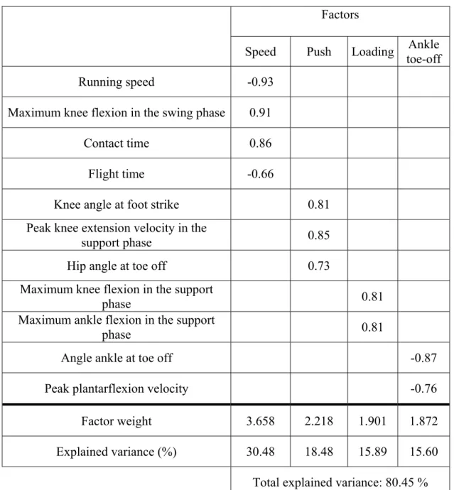
Table 4.1 displays the varimax rotation matrix of components obtained by factor analysis. Ten biomechanical parameters, selected through preliminary analyses, have been included into the analysis together with running speed. Four main components, explaining ∼80% of total variance, can be clearly distinguished.

The first factor has been identified as the “speed” factor, being highly correlated with running speed and contact time, a covariate of running speed. The flight time is also included in this component, although it is less correlated to it due to its non-linear relation vs. running speed (Nummela 2007). Interestingly, the maximum knee flexion during the swing phase is also correlated to this factor. In fact, this angle becomes more acute with increasing speed, probably due to the higher inertial angular velocity at the hip joint.

The second component, explaining 18.48% of total variability is related to two parameters characterizing the push off, i.e. the peak knee extension velocity in the support phase and the hip angle at toe off, therefore it has been characterized as the “push” factor. The knee angle at foot strike is also positively related to this factor.

The third factor, “loading”, is related to two parameters clearly characterizing the loading phase during the support, i.e. the maximum knee and ankle flexion in that phase, occurring about a at the midsupport.

Finally, the fourth component is correlated to the ankle angle at toe off and the peak plantarflexion velocity during the support phase, thus describing the behaviour of the ankle joint at the toe off. Therefore, it has been defined “ankle toe-off”.

4.3.2 Mechanical differences between economical and non-economical

runners

FIGURE 4.1. Oxygen uptake vs. running speed relationship for the 10 runners

(regression lines are obtained interpolating the VO2 values at the four considered

speeds)

The VO2 vs. speed linear relationships for the 10 athletes are shown in fig. 4.1. High

variations in VO2submax may be noted between the more and less economical

athletes at given submaximal speeds, with a range of about 15 ml·min-1·kg-1. Figure 4.2 displays the individual net energy cost of running (C) plotted vs. speed. For some of the athletes C was not constant across speeds but it followed an hyperbolic trend.

This might be expected according to a mathematical deduction. In fact, assuming a linear VO2 vs. speed relationship and considering that C=VO2·speed-1, the C vs. speed

relationship results to be an hyperbola. It is worth nothing that for a subject (marked with white triangles) the intraindividual variation in C across different speeds got up to ∼0.4 ml·kg-1·m-1 (Fig 4.2). 0,16 0,17 0,18 0,19 0,2 0,21 0,22 0,23 0,24 0,25 0,26 10 11 12 13 14 15 16 17 18 19 running speed (km·h-1) C (ml·kg -1 ·m -1 )

FIGURE 4.2. Energy cost of running vs. running speed relationship for the ten

runners (the subjects showing the highest intraindividual variability is marked with empty triangles)

Table 4.1 shows the mean ± SD values of biomechanical parameters for the three groups of athletes subdivided according to their RE in economical, intermediate

and non economical. Several significant differences were revealed by non parametric ANOVAs between the groups.

The maximum knee angle during the support phase (maximum loading knee angle) was significantly lower (i.e. more acute) in economical vs. both intermediate and non-economical runners, such as in intermediate vs. non-economical runners, thus following a trend to decrease with increasing economy. An analogous trend appeared for the total plantarflexion angle during the support phase, being ∼3 degrees higher in economical vs. intermediate and ∼4 degrees higher in economical vs. non-economical runners. Economical (n=12) Intermediate (n=16) Non economical (n=12) Contact time (s) 0.229 ± 0.025 0.224 ± 0.024 0.229 ± 0.025 Flight time (s) 0.124 ± 0.017 0.131 ± 0.017 0.115 ± 0.025 Stride length (cm) 143.3 ± 20.5 153.0 ± 16.9‡ 135.6 ± 17.5

Maximum knee extension before the

foot strike (deg) 159 ± 5.2 157 ± 5.1 ‡ 161 ± 3.2 Maximum knee flexion in the swing

phase (deg) 66 ± 9.6 64 ± 11.3 69 ± 10.0 Maximum knee flexion in the support

phase (deg) 137 ± 2.4 †* 140 ± 2.3 ‡ 142 ± 1.8 Knee angle at foot strike (deg) 156 ± 5.6 154 ± 2.9 ‡ 159 ± 1.7

Knee angle at toe off (deg) 159 ± 2.3 158 ± 3.4 ‡ 161 ± 3.5

Total angular excursion in flexion of

the knee (deg) 93 ± 9.4 93 ± 12.2 93 ± 11.5 Peak knee flexion velocity in the

swing phase (deg·s-1) 575 ± 67.1 585 ± 66.1 576 ± 64.4 Peak knee flexion velocity in the

support phase (deg·s-1) 199 ± 30.9 180 ± 38.6 184 ± 39.5 Peak knee extension velocity in the

swing phase (deg·s-1₎ 601 ± 53.9 572 ± 61.8 594 ± 58.8

Peak knee extension velocity in

support phase (deg·s-1) 209 ± 22.0 180 ± 35.3 189 ± 34.1 (Table 4.2:following on next page)

(Table 4.2 follows) Economical (n=12) Intermediate (n=16) Non economical (n=12) Peak knee linear velocity in the

support phase (m·s-1₎ 3.7 ± 0.52 3.5 ± 0.39 3.5 ± 0.41

Peak knee linear velocity in the swing

phase (m·s-1) 6.6 ± 1.07 6.5 ± 0.92 6.6 ± 0.88 Minimum knee linear velocity in

support (m·s-1) 1.9 ± 0.45 1.9 ± 0.39 2.0 ± 0.43 Maximum hip angle (deg) 39 ± 6.3 41 ± 6.8 40 ± 4.7

Minimum hip angle (deg) 25 ± 4.3 25 ± 4.7 25 ± 3.4

Hip angle at foot strike (deg) 22 ± 4.4 23 ± 3.9 22 ± 2.6

Hip angle at toe off (deg) 27 ± 4.6 27 ± 4.2 25 ± 3.8

Total angular excursion in flexion of

the hip (deg) 65 ± 10.7 65 ± 9.3 65 ± 8.2 Peak hip flexion velocity (deg·s-1) 351 ± 55.3 329 ± 45.1 356 ± 44

Peak hip extension velocity (deg·s-1) 331 ± 52.1 325 ± 44.3 327 ± 34.7

Ankle angle at foot strike (deg) 112 ± 7.1 † 105 ± 2.9 ‡ 110 ± 5.5

Maximum ankle plantar flexion (deg) 95 ± 4.1 95 ± 2.3 96 ± 2.9

Ankle angle at toe off (deg) 132 ± 6.5 127 ± 1.5 128 ± 5.1

Total plantarflexion excursion in

support (deg) 36 ± 4.7 †* 33 ± 3.8 32 ± 6.2 Peak plantar flexion velocity (deg·s-1) 353 ± 26.3 † 329 ± 28.1 326 ± 40.4

Shank angle at foot strike (deg) 4 ± 2.6 † 0 ± 2.2 ‡ 4 ± 2.7

Shank angle at toe off (deg) 43 ± 5.0 45 ± 3.1 ‡ 42 ± 3.2

Speed Factor 0.04 -0.33 0.27

Push Factor 0.14 -0.23 0.32

Loading Factor 0.48 * 0.15 ‡ -0.54

Angle Toe-off Factor 0.48 -0.20 -0.25

TABLE 4.2. Differences in kinematics among three RE groups

(Significant differences [p<0.05] between: *economical vs. non-economical; †economical vs. intermediate; ‡intermediate vs. non-economical)

A different trend was shown for other parameters in which intermediate RE runners were different from non-economical runners, while no significant difference was found for the economical runners vs. the other two categories. That is the case of

stride length (with a difference of even ∼15 cm), the maximum knee extension before the foot strike, the knee angle at foot strike and toe off and the shank angle at toe off.

Furthermore, runners belonging to the intermediate RE category showed a more acute angle ankle at foot strike compared to the other two categories, and a vertical position of the shank at the foot strike while economical and non-economical runners landed with a shank angle of 4 degrees.

A parameter characterizing strictly the economical runners was the peak plantarflexion velocity (353 ± 26.3 deg·s-1), resulting higher than in the intermediate (329 ± 28.1 deg·s-1) and the non-economical (326 ± 40.4 deg·s-1) groups.

Among the factors, only the loading factor showed significant differences between groups: non-economical runners showed a negative value opposed to the positive one of the other two categories. This indicates that non-economical runners had a lower loading during the support phase compared to their more economical counterparts.

4.3.3 Multiple regression

Six biomechanical parameters were finally obtained with a stepwise multiple regression procedure as predictors of VO2submax, i.e. RE. The model is the

following:

VO2= –0,53a – 1,66b + 0,15c + 1,49d – 2,22e – 1,08f + 985,6 with:

a = the hip angle at foot strike b = the hip angle at toe off

c = the peak plantarflexion velocity d = the ankle angle at toe off

e = the maximum ankle flexion during the support phase f = the knee angle at toe off

FIGURE 4.3. Predicted (through the multiple regression model) vs. observed VO2

The model explained ∼72% of RE variability in the considered sample of ten middle-distance runners at four submaximal velocities (Fig. 4.3).

Table 4.3 displays the significance for the coefficients of independent variables. Except that the hip angle at foot strike, all other variables were significant

R

= 0,7227

Predicted VO

(ml·min·kg

)

Actual VO

(ml·min·kg

)

Non standardized coefficients Standardized coefficients t Sig. Collinearity statistics

B _error St Beta Tolerance VIF

Constant 985.56 199.56 4.94 0.00 knee angle at toe off -1.08 0,27 -0.81 6.76 0.00 0.60 1.66 maximum ankle flexion during the support phase -2.22 0.33 -0.81 6.76 0.00 0.48 2.09 ankle angle at toe off 1.50 0.24 0.8 6.22 0.00 0.35 2.86 peak plantarflexion velocity 0.15 0.03 0.59 4.3 0.00 0.37 2.71 hip angle at toe off -1.66 0.32 -0.7 5.25 0.00 0.39 2.58 hip angle at foot strike -0.53 0.27 -0.26 1.92 0.06 0.38 2.64

4.4 Discussion

The present study was designed to test the hypothesis that a significant amount of the intra- and inter-individual variation in RE is accounted for the differences in running technique. The results seem to support this hypothesis, although they require a cautious and careful interpretation due to the extraordinary complexity of the phenomenon under examination.

In the kinematical analysis of economic vs. non-economic athletes, one of the parameters better differentiating the groups of runners was the maximum knee flexion during the support phase. It seems that a more acute knee angle at the mid-support may allow a lower energy expenditure. This is in agreement with the previous study of Williams (1987a). A possible explanation for this lies in the reduction of eccentric force production when braking the body’s falling in the first half of the support phase, causing a lesser energy consumption according to the link between force production and energy requirements (see chapter 5 for a detailed analysis on this). However, it is logical and experimentally proved (McMahon 1987) that excessive knee flexion in the mid-support would result in an higher energy cost of running. Therefore, it is hypothesizable that an optimal knee flexion may exist and further investigation designed to test this hypothesis are needed. The maximum knee flexion in the support phase was highly correlated with the “loading” factor (r=0.81). Then, it is not surprising that this factor too discriminated between RE levels, showing a marked lowering trend across the factorial axis with decreasing RE, up to negative values in non-economical runners.

economical athletes than in their less economical counterparts. This results also are in good agreement with the findings of Williams (1987a), although the data about plantarflexion velocity are in contrast with the previous study of Williams himself (1986), where poor RE was associated with a high peak plantarflexion angular velocity. It is possible that, analogously at the hypothesis done about the knee angle, not excessive rigidity of the musculotendineous system at the ankle (involving higher angular displacements) may result in lower force production and thus energy savage. Instead, there is not an immediate interpretation to the discrepancies among studies. It is possible that the very complex interaction among the mechanical factors may require very high sample sizes to clearly define a phenomenon, and definitive conclusions will be achieved only with large samples, or associating the findings of more subsequent studies. Therefore, the fact that in two similarly designed studies (the present and Williams 1987a) few mechanical parameters resulted related to RE and some of them are the same in the two studies, let deduce that those parameters (e.g. maximum knee flexion, ankle displacement and peak plantarflexion velocity) are really important for RE.

Besides the afore-discussed parameters, other significant differences between the three considered RE levels, i.e. economical, intermediate, and non-economical have been showed in this study. For some of the variables, the extreme value is showed by the intermediate RE group, while economical and non-economical are similar. This is the case of stride length, maximum knee extension before the foot strike, knee angle at toe off and foot strike, ankle angle at foot strike and the shank angle at foot strike and toe off. With this U-shaped behaviour, it is possible that the relationships indicate very few about the absolute importance of the respective

parameters for RE, and that it is the overall interaction of all those factors to be important.

In summary, the analysis of the mechanical differences between economical and non-economical subjects confirmed that very few single parameters (maximum knee flexion during the support, maximum angular displacement of the ankle in the support phase, and peak plantarflexion velocity) may be related to some extent to RE. The factor analysis performed on 11 variables revealed four components that may be considered as global descriptors of the running technique. The high fraction of total variance explained by these four factors (80%) indicates that the multivariate statistical approach is a good tool to discover the interactions between different discrete mechanical parameters, thus obtaining few global descriptors of the running technique. Unfortunately, only one of this factors, the “loading factor” discriminated well between different levels of RE. This indicates that the factor analysis carried out with this number of parameters is not yet sufficient to characterize the profile of an economic runner, and further analysis including more mechanical descriptors are required.

Finally, the good fit of the multiple regression analysis (R2=0.72) confirm that variance in RE may be explained to a great extent by running technique. The remainder of the variance might be related to physiological or other factors not considered in this study. The six parameters included in the model are representative of all the lower limb joints (hip, knee and ankle). Other variables might have been included instead of those chosen with just very little changes of the model fit, confirming that substantially no exclusive biomechanical index is more important to

5.STUDY 2

A MATHEMATICAL MODEL PREDICTING

RUNNING ECONOMY FROM BIOMECHANICAL

PARAMETERS

5.1 Introduction

The relationships between running economy and mechanics may be analysed

a priori considering the biomechanical determinants of energy expenditure during

running.

Several studies in the field of comparative biology and applied physiology have shown that RE is proportional to the rate of average muscular force production during running (Kram 1990, Roberts 1997, Wright 2001, Sih 2003, Biewener 2004, Pontzer 2005, Pontzer 2007). Experimental research revealed that the greatest portion of the muscular force produced during constant speed running is applied to support the runner’s body weight (Kram 1990, Farley 1992, Chang 1999). A significant amount of force, however, is needed to accelerate the runner’s center of mass at each stride (Cooke 1991, Chang 1999) and to swing the oscillating limb (Marsh 2004, Modica 2005).

The purpose of this study is to develop and test a mathematical model predicting RE from the estimated rate of force production on trained competitive athletes. The model considers the three sources of muscular force production during running, namely the vertical and horizontal components of the ground reaction force (GRF) and the force required to swing the limb. The model was adapted from Pontzer

(2005, 2007) which has developed and successfully tested his “Limb” model to predict the energy cost of locomotion in different species of animals and in untrained humans.

5.2 Model derivation

5.2.1 Estimation of GRF

-200

0

200

400

600

800

1000

1200

1400

1600

0

0,05

0,1

0,15

0,2

Time (s)

Force (N)

GRF VERT

GRF HORIZ

In this study the ground reaction forces (GRF) have been estimated from kinematical measures according to theoretically established relationships. The GRFVERT (i.e. vertical component of the GRF) vs. time relationship during stance

(represented by the continuous line in Fig. 5.1) was computed according to a model considering the force as a function of time during contact to be a simple sine function (Alexander 1989):

FVERT(t) = m ⋅ g ⋅ π/2 ⋅ (tf/tc+1) ⋅ sin (π/tc ⋅ t) (1)

being:

m (kg): the runner’s body mass g: the gravity = 9.81 m⋅s-2

tc (ms): the contact time

tv (ms): the flight time

The validity of this postulate has been checked comparing the areas under the modelled and actual force curves obtained with force plates at different speeds: the mean bias between force plateform and modelled force vs. time areas was 2.93% in overground running (Morin 2005).

The mean vertical force (mFVERT) during stance was obtained dividing the

area under the FVERT (t) curve, i.e. the vertical impulse, by the contact time:

mFVERT =

(∫

To relate force production to RE, that is the rate of energy consumption standardized to body mass, a rate of vertical ground force production (mFVERTrate)

was computed by dividing mFVERT by the body mass m and multiplying it by the

stride frequency, sf = (tc+tf)-1:

mFVERTrate= mFVERT⋅m-1⋅sf (3)

Least squares regression was employed to determine the percentage of observed variation in RE values at each of the considered speeds (n= 40, obtained from 10 subjects and four speeds) explained by mFVERTrate.

5.2.2 Estimation of GRF

The GRFHORIZ (i.e. the horizontal component of the GRF) vs. time relationship

during stance (represented by the dotted line in Fig. 5.1) was obtained as follows. Firstly, the limb angle with the vertical at the foot strike (α) was computed through trigonometric relationships (Fig 5.2).

The limb length (L) was measured in the athletes as the vertical distance from the great trochanter to the ground, while the distance travelled by the centre of mass during the stance phase was approximated to d = running speed ⋅ tc. Therefore the α

angle was obtained as α= arcsin (d/2 ⋅ L-1_{). Assuming that the width of the α angle}

(i.e. the angle between the limb and the vertical) is identical at the foot strike and toe off (fig 5.2), and that the limb rotates at a constant angular velocity during the stance phase, it is possible to calculate the instantaneous limb angle (αinst) function of time

during the stance as:

αinst (t) = α ⋅ (2t ⋅ tc-1 -1) (4)

The GRFHORIZ vs. time function was then obtained by multiplying the GRFVERT

function (1) by the tangent of the αinst function (4).

FHORIZ(t) = m ⋅ g ⋅ π/2 ⋅ (tf/tc+1) ⋅ sin (π/tc ⋅ t) ⋅ tan [α ⋅ (2t ⋅ tc-1 -1)] (5)

The mean horizontal force (mFHORIZ) during the propulsive phase of stance was

obtained dividing the area under the FHORIZ (t) curve between tc/2 and tc, i.e. the

impulse, by the half contact time:

mFHORIZ =

(∫

As for GRFVERT, to relate the force production to RE, a rate of horizontal ground

force production (mFHORIZrate), standardized on body mass, was computed by

dividing mFHORIZ by the body mass m and multiplying it by the stride frequency:

mFHORIZrate= mFHORIZ⋅m-1⋅sf (7)

To test the prediction power of the model including both the vertical and horizontal GRF components, a linear combination of mFVERTrate and mFHORIZrate

(mF(HORIZ+VERT)rate) was computed. A coefficient of 4 was attributed to FHORIZ to

account for the worst muscle mechanical advantage of horizontal force production compared to vertical force production (Roberts 1998a, 1998b). The coefficient’s value was established according to the relative contribution of horizontal forces production to the total energy expenditure (Chang 1999).

Thus:

mF(HORIZ+VERT)rate= mFVERTrate+4⋅mFHORIZrate (8)

The percentage of observed variation in RE values at each of the considered speeds explained by mF(HORIZ+VERT)rate was assessed with least squares regression method.

5.2.3 Estimation of the force to swing the limb

The mean force to swing the limb in a stride (FSWING) was computed according

FSWING = m⋅g⋅ML⋅D⋅2α⋅⏐1- (sf/2)-2 T-2⏐ (9)

being:

m(kg): the runner’s body mass g: the gravity = 9.81 m⋅s-2

ML: the limb mass, estimated as 16% of body mass according to Dempster (1955)

D(m): the radius of gyration of the pendulum = 0.56 ⋅ L (Plagenhoef 1966), where L is the limb length

α (rad): the angle between the limb and the vertical at the toe off sf(s-1): the stride frequency = (tc+tf)-1

T(s): the resonant period of the limb = 2π⋅ (0.562 _{⋅ L⋅ g}-1₎0.5 _{(Pontzer 2005)}

FSWING was standardized for body mass (m) and multiplied by stride frequency

(sf) to obtain the rate of production of force to swing the limb (FSWINGrate):

FSWINGrate= FSWING⋅m-1⋅sf (10)

5.2.4 The complete model

A weighted sum of the mean vertical and horizontal components of the ground reaction force and the force to swing the limb was carried out to obtain an estimate of the rate of total force production (FTOTrate):

A coefficient of 30 was attributed to FSWING according to the literature

(Pontzer 2005).

Least squares regression was used to determine the percentage of observed variation in RE values explained by the complete model.

5.3 Results

5.3.1 Testing of partial components

FIGURE 5.3. Mean vertical rate of force production (mFVERTrate) vs. RE

The mean rate of the vertical component of the GRF alone explained a wide part of the inter-individual variability in RE (R2=0.69) (Fig.5.3). If individual subjects were considered (i.e. the model is tested on the four data points of an individual athlete) rather than the whole group, the explained variability in intra-individual RE rose up to R2 = 0.97 - 0.99. R2 = 0,6849 0,5 0,6 0,7 0,8 0,9 1,0 1,1 1,2 35 37,5 40 42,5 45 47,5 50 Force (N·s-1·kg-1) VO 2 (ml·s -1 ·kg -1 )

FIGURE 5.4. Mean vertical + horizontal rate of force production

(mF(HORIZ+VERT)rate) vs. RE

The mean rate of the combined vertical and horizontal forces component of the GRF (mF(HORIZ+VERT)rate) explained a wider part of the variability in RE

(R2=0.79) (Fig.5.3) compared to mFVERTrate.

R

= 0,7928

Force (N·s

·kg

)

VO

(ml·s

·kg

)

5.3.2 Testing of the complete model

FIGURE 5.5. Rate of total force production (FTOTrate) vs. RE

The total model, including all the components of the muscular force produced during running (vertical and horizontal ground reaction forces and the force to swing the limb) explained a high portion of the total variability in RE (R2=0.86) (Fig. 5.5).

R

= 0,8622

0,5

0,6

0,7

0,8

0,9

1,0

1,1

1,2

80

90

100

110

120

130

140

150

Force (N·s

·kg

)

VO

(ml·s

·kg

)

5.4 Discussion

The purpose of this study was to develop and test a mathematical model predicting RE from the rate of force production during running, estimated with kinematical parameters.

The first parameter that have been related to RE is the rate of vertical ground reaction force production (mFVERTrate): it explained the 68% of the total variability in

submaximal VO2 (Fig 5.3), a value close to that reported in literature for non

competitive human subjects (Pontzer 2007). It should be noted that equation to obtain mFVERTrate (equation 3, pag. 42) may be algebraically simplified to mFVERTrate = g⋅

tc-1, where g is the gravity and tc the contact time. Therefore, mFVERTrate depends

only on tc in level running at constant speed. Thus, a longer stance phase,

independently from speed, flight time and stride frequency, allows a lower energy expenditure according to the relationship. The high portion of total variability in RE explained here by tc on a sample of competitive middle-distance runners confirms that

the force of supporting the runner's weight and the time course of generating this force is a major determinant of the cost of running (Kram 1990).

It is worth noting that the fit of the model is largely influenced by inter-individual differences in the constant relating mFVERTrate to the submaximal VO2, i.e.

the slope of the mFVERTrate vs. VO2 relationship (Fig. 5.3). In fact, when

intra-individual analyses were performed considering the same relationships in each single athlete, the data points of each velocity were almost aligned. The same is true also when the horizontal GRF and FSWING are included in the model. Then, a great portion

analogous phenomenon was observed by Pontzer (2005, 2007) and Weyand (2001). Individual characteristics not included in the model such as fibre type composition, the capacity to store and recovery elastic energy and the muscle mechanical advantage may be responsible to the variation in the individual force production/energy consumption ratio, and further studies are needed to investigate on this.

The model fit improved (explaining 79% of total variability in RE) including the cost for generating horizontal (braking) ground reaction forces (Fig. 5.4). This means that despite the logical correlation between mFVERTrate and mFHORIZrate (the

second parameter is obtained by the first, eqs. 4-7), a certain variability in FHORIZ is

independent from FVERT.

It should be noted that in the present study FHORIZ was estimated differently

than in the study from which the model have been adapted (Pontzer 2005). In that work, average FHORIZ was simply approximated to mean FVERT multiplied by the

tangent of the limb angle with the vertical at toe off. This assumes that the mean tangent of several angles is equal to the tangent of the mean of those angles, that is not the case! Therefore, in the present study the instantaneous limb angle function of time during the stance was considered (equation 4, pag. 43) although this involved enormous complications in the calculation of primitives.

A rationale to the interaction of horizontal and ground reaction forces to influence RE during level running at a given speed may be given considering the relationships between stance duration (tc) and the braking-propulsion phases at each

speed. While a long tc is advantageous for a lower energy cost, it implies that the

angle with the vertical (α, see Fig. 5.2) and increasing the horizontal ground reaction force (eq. 5). Probably optimal values of tc and α exist such that mF(HORIZ+VERT) rate

and thus the energy consumption is minimized at a given speed, assuming a constant limb length. Further studies are needed to test this hypothesis, although the computation of that value appears far from being simple.

The complete model, including the force to swing the limb, explained a greater part of total variability in RE: 86% (Fig. 5.5). This means that the model works very well to predict running economy from rate of force production also in trained competitive runners and it gives further support to the force production hypothesis of a direct relationships between the force produced and the energy consumed during running (Kram 1990, Taylor 1994). As previously observed, a greater part of the reminder variability may be attributed to inter-individual variations in the constant relating the force produced and VO2.

In summary, this study showed that running economy may be successfully predicted in competitive runners by the rate of muscular force production during running, estimated with mathematical modelling.