Atomic Force Microscopy Studies of the Amyloidogenic Processes of Intrinsically Unstructured Proteins related to Neurodegenerative Diseases

A

A

l

l

m

m

a

a

M

M

a

a

t

t

e

e

r

r

S

S

t

t

u

u

d

d

i

i

o

o

r

r

u

u

m

m

–

–

U

U

n

n

i

i

v

v

e

e

r

r

s

s

i

i

t

t

à

à

d

d

i

i

B

B

o

o

l

l

o

o

g

g

n

n

a

a

DOTTORATO DI RICERCA IN

CELLULAR, MOLECULAR AND INDUSTRIAL BIOLOGY

Ciclo:

XXIV

Settore Concorsuale di afferenza:

BIOLOGICAL, BIOMEDICAL AND

BIOTECHNOLOGICAL SCIENCES

TITOLO TESI

ATOMIC FORCE MICROSCOPY STUDIES OF THE AMYLOIDOGENIC PROCESSES OF

INTRINSICALLY UNSTRUCTURED PROTEINS RELATED TO NEURODEGENERATIVE

DISEASES

Presentata da:

DHRUV KUMAR

Coordinatore Dottorato

Relatore

Tutore

PROF. VINCENZO SCARLATO

PROF. BRUNO SAMORI

DR. MARCO BRUCALE

Atomic Force Microscopy Studies of the

Amyloidogenic Processes of Intrinsically

Unstructured Proteins Related to

Neurodegenerative Diseases

By

Dhruv Kumar

Ph.D. Cycle-XXIV

PhD School in Biological, Biomedical, and Biotechnological Sciences

PhD program in Cellular, Molecular, and Industrial Biology

NanoBiotechnology and NanoBioscience lab

Department of Biochemistry,

University of Bologna, Italy

PhD Supervisor: Prof. Bruno Samori (PhD) PhD Co-supervisor: Dr. Marco Brucale (PhD) PhD Coordinator: Prof. Vincenzo Scarlato (PhD)

“You have to dream before your dream can come true”

Abdul kalam

Abstract

Protein aggregation and formation of insoluble aggregates in central nervous system is the main cause of neurodegenerative disease. Parkinson’s disease is associated with the appearance of spherical masses of aggregated proteins inside nerve cells called Lewy bodies. α-Synuclein is the main component of Lewy bodies. In addition to α-synuclein, there are more than a hundred of other proteins co-localized in Lewy bodies: 14-3-3η protein is one of them. In order to increase our understanding on the aggregation mechanism of α-synuclein and to study the effect of 14-3-3η on it, I addressed the following questions. (i) How α-synuclein monomers pack each other during aggregation? (ii) Which is the role of 14-3-3η on α-synuclein packing during its aggregation? (iii) Which is the role of 14-3-3η on an aggregation of α-synuclein “seeded” by fragments of its fibrils?

In order to answer these questions, I used different biophysical techniques (e.g., Atomic force microscope (AFM), Nuclear magnetic resonance (NMR), Surface plasmon resonance (SPR) and Fluorescence spectroscopy (FS)).

To answer the first question, I compared by AFM imaging the in vitro aggregation of α-synuclein with that of α-α-synuclein dimers (NC-, NN-, and CC-terminal dimers) and with that of a so-called Synucle-Nuclein construct. The Synucle-Nuclein construct is a dimer where an α-synuclein moiety lacking N-terminal region (Synucle) is connected to another moiety of α-synuclein lacking C-terminal region (Nuclein). In this construct the two NAC (Non Amyloid-beta Component) regions that drive the formation of β-sheet like structure in the fibrils are tethered together, contrary to the cases of the other three dimers. I found that only the NC-terminal dimer aggregates into mature fibrils like α-synuclein does, whereas both NN- and CC-terminal dimers form amorphous aggregates. Also the Synucle-Nuclein construct aggregates into mature fibrils, but they are shorter in length than those of α-synuclein. This is a strong indication that in α-synuclein fibrils the monomer moieties are packed in a head to tail fashion, and that the NAC β-sheet packing is the core of the fibrils.

To answer the second question, I studied the in vitro aggregation of synuclein and α-synuclein dimers in the presence of different molar concentration of 14-3-3η. Imaging with AFM, I found that 14-3-3η affects the aggregation pathway of α-synuclein by modifying the shape of the growing oligomers and protofibrils. NMR and SPR revealed that 14-3-3η does not interact with α-synuclein monomer. AFM showed that 14-3-3η does not interact also with α-α-synuclein mature fibrils. In order to prove that 14-3-3η targets the oligomeric species, I labeled both α-synuclein and 14-3-3η with a fluorophore, and by FS I could demonstrate that 14-3-3η intercalates into the

was confirmed by the data obtained on trying to answer the third question, when I studied α-synuclein aggregation in the presence of both 14-3-3η and fragments of α-α-synuclein mature fibrils. These fragments were prepared by ultrasonication of α-synuclein mature fibrils. By exposing their “living ends”, they can favor and “seed” the aggregation of monomeric α-synuclein. Imaging with AFM, I found that 14-3-3η slows down the addition of monomeric α-synuclein to the exposed living ends of those seeds. These AFM data on the growth of α-synuclein seeds in the presence of 14-3-3η and those obtained by FS on the inclusion of 14-3-3η into the growing oligomers and fibrils of α-synuclein demonstrate that the 14-3-3η can inhibit the α-α-synuclein aggregation by an intercalation mechanism. This capability might explain the co-localization of 14-3-3η and α-synuclein in Lewy bodies.

Key words:

Acknowledgements

Firstly, I would like express my deepest gratefulness to my principle supervisor, Prof. Bruno

Samori for providing me an exciting research project and research environment. He has been a

great mentor and I am deeply grateful for all the encouragement, guidance, support and love he has provided over the last three years. I would like to express my great gratitude to my co-supervisor

Dr. Marco Brucale for providing me a stimulating and enjoyable environment to work in and great

support throughout my Ph.D. I would like to give thank to my PhD coordinator Prof. Vicenza

Scarlato for coordinating PhD program, and available always for the project discussion and for

help. Thanks are also given to all other colleagues and friends (Prof. Giampaolo, Daniele,

Alixendera, Rosita, Massimo, Aldo, Danial, Manuele, Simone, Silvia, Francesca, Federica, Andrea and others) at Samori lab (Nanobioscience lab) for their support, discussion and

encouragements.

I am also thankful to the Ministry of external affairs (MHRD) India and Italy for providing me partially financial support during my PhD and Institute of advanced studies (Brain’s in competition program), Bologna, Italy for providing me free accommodation throughout my Ph.D.

I would like to thank our project collaborators (Prof. Luigi Bubacco, laura, Isabella,

Nicoletta and Marco) at the Molecular Biology lab, University of Padova for providing me protein

samples (α-Synuclein and 14-3-3 protein) for the single molecule and aggregation experiments and

Prof. Hilal lashuel at laboratory of molecular and chemical biology of neurodegeneration, EPFL,

Lausanne for providing me amyloid beta protein.

I would like to thank my friends (Saurabh, Deepak, Prashant, S.M. Velu, Rashmi, Priyank

Shukla, and Shalini Tiwari) who always encouraged me and boost me to work hard.

I would like to thank Prof. Dwijendra K. Gupta for his great support and encouragement throughout my Ph.D.

I would like to thank Prof. Paolo Neyroz at department of Pharmacy, University of Bologna for providing me Fluorescence polarization spectroscope and Dr. Marzia Govoni at department of virology, University of Bologna for providing me Ultrasonic Sonicator.

Finally, I express my warmest gratefulness and love to my parents, my younger brother (Dhanesh), my sweet heart wife and my lovely little master (Karamveer) to whom I am deeply indebted for their constant words of encouragement, love, moral support and happiness.

Declaration

I, Dhruv Kumar confirm that the research work presented in this thesis is my own. Where information has been derived from other sources, I confirm that this has been indicated in the thesis.

List of abbreviation

CD: _{Circular dichroism}

CM-AFM: _{Contact mode atomic force microscopy} CNS: _{Central nervous system}

DLB: _{Dementia with lewy bodies} DTT: _{Dithiothreitol}

FP: _{Fluorescence polarization} GAGs: _{Glycosaminoglycans} HD: _{Huntington disease}

HPLC: _{High performance liquid chromatography} HTT: _Huntingtin

LBD: _{Lewy body disease} LBs: _Lewy-bodies LNs: _{Lewy neurites}

MSA: _{Multiple system atrophy} NAC: _{Non amyloid component}

NCM-AFM: Non-contact mode atomic force microscopy NMR: _{Nuclear magnetic resonance}

PBS: _{Phosphate buffered saline} PD: _{Parkinson’s disease} PMDs: _{Protein misfolded diseases} PrPSc: _{Prion protein}

PS1: _{Presenilin 1}

PSP: _{Progressive supranuclear palsy}

SDS-PAGE: Sodium dodecyl sulfate polyacrylamide gel electrophoresis SEM: _{Scanning electron microscope}

SOD1: _{Superoxide dismutase-1} STM: _{Scanning tunneling microscope} SUVs: _{Small unilamellar vesicles}

TEM: _{Transmission electron microscope} TM-AFM: Tapping mode atomic force microscopy WT: _{Wild type}

List of figures

Figure 1.1: Model for protein misfolding and fibrillization………...…6

Figure 1.2: Working principle of tapping mode atomic force microscopy……….….9

Figure 1.3: Non-contact mode atomic force microscope……….12

Figure 1.4: A typical AFM force curve……….………..17

Figure 1.5: Scheme showing polarization of plane polarized light by fluorescent molecule in fluorescent polarization experiment………...20

Figure 1.6: The human synuclein family………23

Figure 1.7: Schematic representation of primary structure of α-synuclein………...25

Figure 1.8: Putative pathological mechanisms of α-synuclein………...…………...…… 29

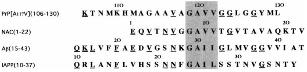
Figure 1.9: Comparison of NAC with Aβ, PrP, and IAPP sequences………..31

Figure 1.10: Model of disease pathway in Parkinson’s disease………..….35

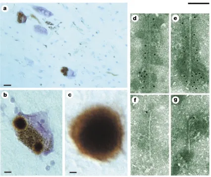
Figure 1.11: The α-synuclein pathology of Parkinson’s disease………...…...….. 36

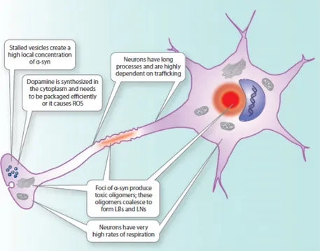
Figure 1.12: Summary schematic of α-synuclein toxicity in a dopaminergic neuron………..….37

Figure 1.13: Alignment of α-synuclein and the 14-3-3 family of proteins………...……….39

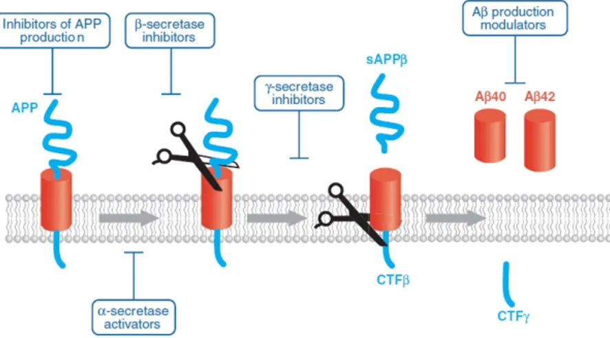
Figure 1.14: Aβ production………..42

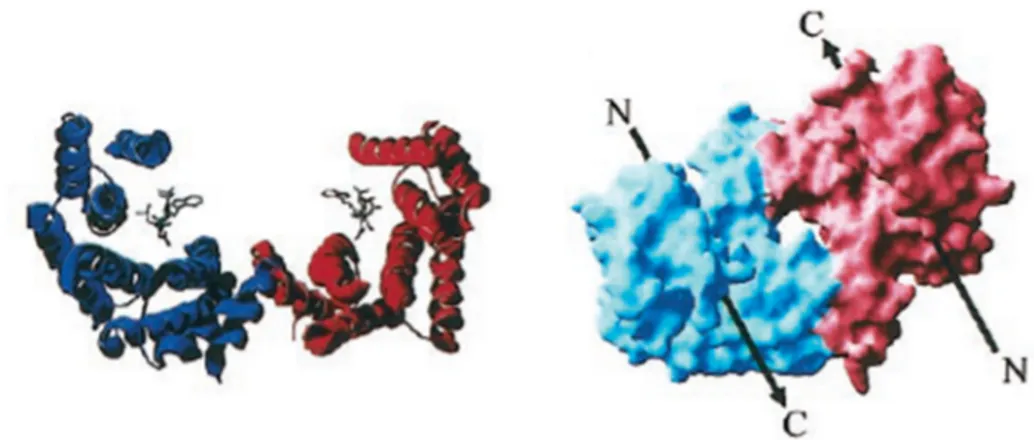
Figure 1.15: Crystal structure of 14-3-3 η dimer………...…44

Figure 1.16: Crystal structural model of 14-3-3ζ………..46

Figure 1.17: Multiple sequence alignment of α-synuclein and 14-3-3η showing alignment score 47...52

Figure 1.18: Multiple sequence alignment of 14-3-3γ and 14-3-3η………..53

Figure 2.1: AFM image analysis of early-formed α-synuclein oligomers………..….55

Figure 2.2: AFM image analysis of belatedly-formed α-synuclein oligomers……….56

Figure 2.3: AFM image analysis of non-spherical α-synuclein oligomers……….57

Figure 2.4: AFM image analysis of α-synuclein protofilaments……….……..58

Figure 2.5: AFM image analysis of α-synuclein protofibrils……….…..59

Figure 2.6: AFM image analysis of α-synuclein mature fibrils………...…..60

Figure 2.7: Model of the hierarchical structure and the roles of the terminal regions in the assembly of α-synuclein fibril……….………..61

Figure 2.8: AFM image analysis of α-synuclein mature fibrils induced by seeds………..63

Figure 2.9: AFM image analysis of NN-terminal dimer………..…..64

Figure 2.10: AFM image analysis of CC-terminal dimer………..…………66

Figure 2.13: AFM image analysis of Aβ mature fibrils……….…….71 Figure 2.14: NMR analysis of interaction between α-synuclein and 14-3-3η………..…..72 Figure 2.15: SPR analysis of interaction between α-synuclein and 14-3-3η………...………73 Figure 2.16: AFM image analysis of α-synuclein mature fibrils obtained in the presence and absence of

14-3-3η………..…….74

Figure 2.17: AFM image of curved object obtained during α-synuclein aggregation in the presence

14-3-3η by following different stoichiomeric ratio………...75

Figure 2.18: Height and curvature distribution of curved object following different stoichiometric

ratio of 14-3-3η and α-synuclein (1:1, 1:4, 1:7, 1:12, 1:20, 1:24, 1:30 1:∞)………...………76

Figure 2.19: AFM image of immunogold labeled curved object α-synuclein with 14-3-3η in the

presence of 14-3-3η specific antibody………78

Figure 2.20: TEM image analysis of immunogold labeled curved objects in the presence of 14-3-3η

specific antibody………...……79

Figure 2.21: Fluorescence emission spectra of α-synuclein aggregates………....79 Figure 2.22: Fluorescence spectra of curved object binding with ThT………...………80 Figure 2.23: AFM image of seeded growth of α-synuclein aggregation suppressed by 14-3-3η……..….81 Figure 2.24: AFM image of curved object obtained during the NC-terminal dimer aggregation in the

presence 14-3-3η………..……82

Figure 2.25: AFM image of curved object obtained during the amyloid-beta aggregation in the

presence 14-3-3η………..83

Figure 2.26: AFM image of α-synuclein aggregation unaffected by 14-3-3γ dimer………...……83 Figure 2.27: AFM image of seeded growth of α-synuclein aggregation unaffected by 14-3-3γ……...…..84 Figure 3.1: General scheme of WSXM showing the most representative process………...……...….88

List of tables

Table 1.1: Common neurodegenerative diseases characterized by deposition of aggregated

proteins………....5-6

Table 1.2: Physical methods used in the literature to analyze protein aggregation………8 Table 1.3: Milestones in 14-3-3 research……….………...…48-49

Publication arising from the thesis

1. Chaperone like protein 14-3-3η interacts with human α-synuclein aggregation

intermediates rerouting the intracellular amyloidogenic pathway – Manuscript Under

preparation.

2. Structure and aggregation of α-Synuclein covalent tandem dimers – Manuscript Under preparation.

Contents table

Chapter-1 (Introduction)

[1.1] Protein misfolding in neurodegenerative disease………...2-7 [1.1.1] Role of misfolded proteins in neurodegenerative disease………...2-3 [1.1.2] Mechanisms of protein misfolding……….………..3-4 [1.1.3] Protein misfolding in the presence of seeds………...…4-4 [1.1.4] Protein aggregation in neurodegenerative disease………5-5 [1.1.5] General mechanisms of brain amyloid formation………....……...6-7 [1.2] Biophysical techniques………..7-22 [1.2.1] Atomic force microscope……….…9-19 [1.2.1.1] Atomic force microscopy ………..……….10-10 [1.2.1.2] Mode of operation………10-13 [1.2.1.3] AFM as an imaging device………...13-14 [1.2.1.4] Imaging conditions………..14-15 [1.2.1.5] Choice of probe and substrate………..…15-15 [1.2.1.6] Force spectroscopy……….…16-16 [1.2.1.7] Anatomy of a force curve……….16-17 [1.2.1.8] AFM calibration………...17-18 [1.2.1.9] AFM vs other imaging technique……….18-18 [1.2.2] Fluorescence polarization………...….18-22 [1.3] α-Synuclein……….22-40 [1.3.1] Historical overview………..22-22 [1.3.2] Synuclein family………...22-24

[1.3.3.1] α-Synuclein as an intrinsically disordered protein……….…25-25 [1.3.3.2] Conformational equilibria in α-synuclein...25-28 [1.3.4] α-Synuclein aggregation………28-33 [1.3.4.1] Role of partial folded structure in aggregation or fibril formation………28-28 [1.3.4.2] Mechanism of α-synuclein aggregation………..28-30 [1.3.4.3] Aggregation of α-synuclein fragments………....…30-31 [1.3.4.4] α-Synuclein mutants………..…31-31 [1.3.4.5] Seeded growth of α-synuclein………..32-32 [1.3.4.6] Factors affecting α-synuclein aggregation………32-32 [1.3.4.7] Proteins inhibiting α-synuclein aggregation………...…33-33 [1.3.5] α-Synuclein and neurodegenerattive disease………..33-38 [1.3.5.1] α-Synuclein and parkinson’s disease………..….35-36 [1.3.5.2] α-Synuclein toxicity………....36-38 [1.3.6] α-Synuclein interacting molecules………..38-40 [1.3.6.1] α-Synuclein shares physical and functional homology with 14-3-3 proteins………..39-40 [1.4] Amyloid-beta (Aβ)……….40-42 [1.4.1] Amyloid-beta in neurodegenerative disease………41-42 [1.5] 14-3-3 Proteins………42-53 [1.5.1] General properties………43-43 [1.5.2] Structural basis………...43-47 [1.5.2.1] 14-3-3 monomer contains a conserved amphipathic groove…………...…43-45 [1.5.2.2] 14-3-3 dimer can simultaneously bind two ligands………...46-47 [1.5.3] Disease associated with 14-3-3 proteins………47-49 [1.5.4] Co-localization of 14-3-3 protein in Lewy- bodies………50-51 [1.5.5] Sequence similarity between 14-3-3η and α-synuclein………..…..52-52 [1.5.6] Sequence similarity between 14-3-3 η and 14-3-3γ………53-53

Chapter-2 (Results and Discussion)

Morphological Analysis of Proteins

[2.1] α-Synuclein……….…………55-62 [2.1.1] Monomer……….…………55-55

[2.1.2] Oligomers………55-57 [2.1.3] Morphologically distinct oligomers………..………….57-58 [2.1.4] Protofilaments……….………58-58 [2.1.5] Protofibrils……….58-59 [2.1.6] Mature fibrils………59-62 [2.2] Seeded growth of α-synuclein………..………..62-64 [2.3] α-Synuclein dimers and constructs……….64-70 [2.3.1] NN-terminal dimer………...…………64-65 [2.3.2] CC-terminal dimer………...………65-67 [2.3.3] NC-terminal dimer………67-68 [2.3.4] Synucle-Nuclein constructs……….………68-70 [2.4] Amyloid-beta (Aβ) aggregation……….………...……….70-71 [2.5] Effect of 14-3-3η on α-synuclein aggregation………..71-83 [2.5.1] Interaction between 14-3-3η and α-synuclein monomer……….…………71-73 [2.5.2] Effect of 14-3-3η on α-synuclein mature fibrils………..………73-74 [2.5.3] Effect of 14-3-3η on α-synuclein oligomers………..74-81 [2.5.4] Effect of 14-3-3η on seeded growth of α-synuclein aggregation………..81-81 [2.5.5] Effect of 14-3-3η on NC-terminal dimer………..………82-82 [2.5.6] Effect of 14-3-3η on Aβ aggregation………..………82-83 [2.6] Effect of 14-3-3 γ on α-synuclein aggregation………..…83-84 [2.6.1] Effect of 14-3-3 γ on α-synuclein aggregation……….…………83-84 [2.6.2] Effect of 14-3-3 γ on seeded growth of α-synuclein aggregation……….…84-84

Chapter-3 (Materials and Methods)

[3.1] Cloning, expression and purification………...86-86 [3.2] Atomic force microscopy …………..………...86-89 [3.2.1] Protein aggregation………..86-86 [3.2.2] Sample preparation………..86-86 [3.2.3] AFM imaging……….86-87 [3.2.4] AFM image analysis………..87-89 [3.2.5] Fibril formation and preparation for ultrasonication experiment………..89-89

Chapter-4 (Conclusions)

[4.1] Conclusions ……….………..91-92

Bibliography

Chapter-1

(Introduction)

Neurodegenerative disease is a group of brain related disorder. They involve in the damage and death of neuronal cells in nervous system associated with the protein misfolding and aggregation, which affect the normal function of human brain. In general, neuronal cell death and damage originates by the aggregation of misfolded proteins into the beta sheet like structure in the nervous system. There are several factors that influence the aggregation and accumulation of misfolded proteins into the beta sheet like structure, whereas the exact relation between protein aggregation and and cell death is still not very well understood.

[1.1] Protein misfolding in neurodegenerative disease

Most of the neurodegenerative diseases are associated with the misfolding of intrinsically unstructured proteins into β-sheet like structures. The intrinsically unstructured proteins acquire different conformations when they aggregate to form β-sheet like structure [Sandal et al., 2008]. These conformations are stabilized by the intermolecular interactions, leading to the formation of oligomers, proto-fibrils and fibrils, and finally mature fibrils accumulate as amyloid deposits in affected tissues [Soto et al., 2003; Soto et al., 2008]. Aggregates of amyloid-beta (Aβ) in alzheimer’s disease (AD) and prion protein (PrPSc) in prion diseases accumulate extracellularly, and other misfolded aggregates accumulate intracellularly, such as α-synuclein in parkinson’s disease (PD), superoxide dismutase (SOD) in amyotrophic lateral sclerosis (ALS), tau in tauopathies or AD, and huntingtin (HTT) in huntington disease (HD) [Soto, 2003].

[1.1.1] Role of misfolded proteins in neurodegenerative disease

Over the past two decades misfolded proteins have been widely considered to be the triggering factors in the neurodegenerative disease (e.g. PD, AD, HD, Prion Disease etc.). Perhaps the most convincing pieces of evidence in favor of this observation came from genetic studies. Most of the neurodegenerative diseases mainly arise sporadically, without detectable genetic origins; however, a portion (usually small) of the cases can be inherited (e.g. A30P, E46K, A53T mutations in α-synuclein). Interestingly, mutations in the genes encoding the protein component of the misfolded aggregates have been shown to be genetically associated with inherited forms of the disease [Selkoe et al., 1996; Buxbaum et al., 2000; Hardy, 2001; Soto, 2001]. The familial forms usually have an earlier onset and higher severity than sporadic cases. Mutations in the respective misfolded proteins have been associated with familial forms of many diseases, including PD, AD, HD, ALS and various rarer amyloid-related diseases such as cerebral haemorrhage with amyloidosis of the dutch

Buxbaum et al., 2000; Hardy,2001; Soto, 2001]. The fact that mutations in the genes encoding the misfolded proteins produce inheritable disease is by itself a very strong argument for a crucial role of protein misfolding in the disease.

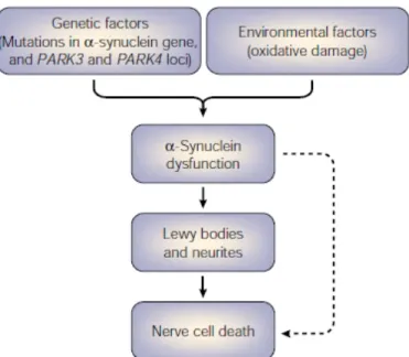
Other evidence for the important role of protein misfolding came from the studies aiming to generate transgenic animal models for protein misfolded diseases (PMDs). Insertion of human genes encoding mutant proteins with a high propensity to misfold and aggregate leads to the emergence of several pathological hallmarks of the different diseases. Human α-synuclein gene expression in transgenic mice induces some of the hallmarks of PD, as dopaminergic cell loss, Lewy-body accumulation and motor dysfunction [Meredith et al., 2008]. In case of prion protein, mice generate spontaneous neurodegeneration accompanied by brain vacuolization as happens in natural transmissible spongiform encephalopathy (TSEs) [DeArmond et al., 1995]. In the case of AD, the most common transgenic models over-express the amyloid precursor protein (APP) and/or the presenilin 1 (PS1), both genes associated to familial forms of AD [Selkoe 1996]. Transgenic mice expressing human mutated APP show amyloid plaques, cognitive impairment, cell death and related inflammatory processes [Duyckaerts et al., 2008]. All these findings suggest that misfolding and aggregation of amyloid proteins play an essential role in the pathology and could be the main cause of Neurodegenerative disease.

[1.1.2] Mechanisms of protein misfolding

Protein misfolding arises from the imperfect folding process that results in the formation of the proteins with different conformations from its native state [Sandal et al., 2008]. Protein misfolding can go on by several reasons [Soto, 2001; Kelly, 1996]. (i) Somatic mutations in the gene sequence leading to the production of a protein unable to adopt the native folding. (ii) Errors on the processes of transcription or translation leading to the production of modified proteins unable to properly fold. (iii) Failure of the folding and chaperone machinery. (iv) Mistakes on the post-translational modifications or trafficking of proteins. (v) Structural modification produced by environmental changes. (vi) Induction of protein misfolding by seeding and cross-seeding mechanisms.

The most common destiny for misfolded proteins is self-aggregation, because the mistaken exposure of fragments to the solvent that are normally buried inside the protein, lead to a high degree of stickiness. The β-sheet structural motif offers the most favorable organization for these intermolecular aggregates and can accommodate an almost unlimited number of polypeptide chains [Kelly, 1996; Nelson et al., 2005]. As a result, misfolded proteins exist as a large and

heterogenous range of polymeric sizes, which are usually classified in very well defined categories, such as oligomers, protofibrils and fibrils [Caughey et al., 2003; Glabe, 2006; Walsh et al., 2007]. Soluble oligomers are small assemblies of misfolded proteins that are present in the buffer soluble fraction of tissue extracts and usually include structures ranging in size from dimers to 24-mers [Glabe, 2006; Walsh et al., 2007]. Recent undeniable facts coming from several autonomous studies of different proteins indicates that oligomers might be the most toxic species in the misfolding and aggregation pathway [Caughey et al., 2003; Glabe, 2006; Walsh et al., 2007]. Protofibrils are larger aggregates that can be seen by using electron microscopy and atomic force microscopy as curvi-linear structures of 4–11 nm diameter and <200 nm long [Caughey et al., 2003; Walsh et al., 1999]. Protofibrils increase in size with increased time and protein concentration, and are lengthened by growth on their ends [Harper et al., 1999]. Annular protofibrils are pore-like assemblies that accumulate in the cell membrane and may contribute to cell death [Srinivasan et al., 2004; Lashuel et al., 2002]. Protofibrils and annular protofibrils have also been shown to be highly toxic in various

in vitro studies [Lashuel et al., 2002; Hartley et al., 1999]. Amyloid fibrils are long, straight and

unbranched structures of around 10 nm diameter and usually several micrometers lengths [Nelson et al., 2005]. They bind the dies Congo red and thioflavin and show a typical “cross-β” X-ray diffraction pattern consisting of two major reflections at 4.7 Å and 10 Å found on orthogonal axes [Nelson et al., 2005]. Fibrils can also elicit toxicity in cultured cells, but usually at much higher concentrations than oligomers and protofibrils [Caughey et al., 2003].

[1.1.3] Protein misfolding in the presence of seeds

The mechanism of protein misfolding and aggregation in the presence of seeds (fragmented mature fibrils) is called as “seeding-nucleation” model [Soto et al., 2006; Jarrett et al., 1993]. In this process, the early steps of misfolding are thermodynamically unfavorable and progress gradually, until the minimum stable oligomeric unit is formed, then grows exponentially at a fast speed. There are two kinetic phases in the seeding-nucleation model of polymerization. Firstly, during the lag phase, a low amount of misfolded and oligomeric structures are produced in a slow process, generating seeds for the next step. Once nuclei are formed, the elongation phase takes place and results in fast growing of the polymers. The addition of pre-formed seeds can reduce the length of the lag phase, accelerating the exponential phase. Fragmented fibrils are considered as the best seeds to propagate the misfolding process in an exponential manner.

[1.1.4] Protein aggregation in neurodegenerative disease

Protein aggregation is the principle phenomena of amyloid like proteins in neurodegenerative diseases such as PD, AD and Prion disease. The rate of morbidity and mortality is higher in the developed world [Hebert et al., 2001; Hebert et al., 2003]. Largely as a result of increased life expectancy and changing population demographics, neurodegenerative dementias and neurodegenerative movement disorders are becoming more common [Brookmeyer et al., 1998; Samii et al., 2004]. Converging lines of investigation have revealed a potential single common pathogenic mechanism underlying many diverse neurodegenerative disorders (i.e., the aggregation and deposition of misfolded proteins). As summarized in Table 1.1, nearly every major neurodegenerative disease is characterized pathologically by the insidious accumulation of insoluble filamentous aggregates of normally soluble proteins in the central nervous system (CNS). Because these filamentous aggregates display the ultrastructural and tinctorial properties of amyloid (i.e., 10 nm wide fibrils with crossed β-sheet structures), these diseases can be grouped together as brain amyloidoses.

From a pathological point of view, neurodegenerative entities are defined by the type and pattern of amyloid deposition in the brain. Unfortunately, the type and pattern of brain amyloidosis does not always correlate well with the observed clinical phenotype. This disconnect has led to a confusing nosology that sometimes requires clinicians to describe phenotypes on the basis of the presumed presence of pathological lesions (e.g., dementia with Lewy bodies) and sometimes requires pathologists to describe lesions using clinical language regardless of the patient’s actual clinical presentation (e.g., progressive supranuclear palsy, PSP). The best way to circumvent this chaos may be the use of chemical analytes of biological fluids and neuroimaging biomarkers that allow clinicians to distinguish between these related brain amyloidoses on the basis of the nature and extent of the brain pathology as well as the specific amyloidogenic protein(s) involved in disease pathogenesis.

Recognizing that all these related neurodegenerative diseases share common mechanisms involving CNS accumulation of misfolded proteins suggests that these disorders may have similar targets for the development of diagnostic and therapeutic agents.

Table 1.1: Common neurodegenerative diseases characterized by deposition of aggregated proteins

Neurodegenerative Disease Related Proteins

Alzheimer’s disease Amyloid-β (Aβ), α-Synuclein, Tau Amyotrophic lateral sclerosis Superoxide dismutase-1 (SOD1)

Cortical basal degeneration/Progressive supranuclear palsy

Tau

Dementia with Lewy Bodies α-Synuclein

Huntington disease Huntingtin (containing polyglutamine repeat expansion)

Multiple system Atrophy α-Synuclein Parkinson’s disease α-Synuclein

Pick’s disease Tau

Prion diseases Protease-resistant prion protein (PrP) Spinocerebellar ataxia Ataxin (containing polyglutamine repeat

expansion)

[1.1.5] General mechanisms of brain amyloid formation

Brain amyloidosis begins with the production of a soluble native protein that is misfolded to yield the precursor for fibril formation (Figure 1.1). The misfolded protein can self-aggregate to form oligomers, protofibrils, or other intermediates that promotes fibril formation [Caughey et al., 2003]. Oligomers of Aβ can be detected in vitro [Huang et al., 2000], in cell culture and transgenic mouse models of Alzheimer’s disease [Walsh et al., 2000; Podlisny et al., 1998; Takahashi et al., 2004], and in postmortem Alzheimer’s disease brain specimens [Kayed et al., 2003].

Figure 1.1: Model for protein misfolding and fibrillization. Soluble native protein is misfolded and

Although, oligomers of α-synuclein have been studied very well, it is obvious that other amyloidogenic proteins such as Aβ or polyglutamine-containing proteins can also form oligomers. Remarkably, oligomers composed of each of these amyloidogenic proteins (which share no primary sequence homology) show a similar conformation-dependent structure [Kayed et al., 2003]. These studies may suggest a common mechanism of amyloid formation that depends upon structural determinants within the oligomers. Further support of this hypothesis, the observation comes from the different forms of amyloid that interact with each other in vitro. For example, α-synuclein can initiate fibrillization of tau, and co-incubation of tau and α-synuclein synergistically promotes fibrillization of both proteins [Giasson et al., 2003].

There are various factors that influence the balance between native protein, misfolded protein, oligomers, and fibrils both in vivo and in vitro. For example, in the disease state, overproduction of the amyloidogenic protein constituent, wrong covalent bond modification, failed degradation, or insufficient molecular chaperone activity may all contribute in shifting the balance towards misfolded protein and oligomer formation. Each of these steps represents a potential target for therapeutic intervention, with therapies being developed currently for different forms of amyloid.

[1.2] Biophysical techniques

There are several techniques that can be used for the study of protein aggregation and its characterization. Eeach techniques have their own advantages and disadvantages. These techniques are summarized in Table 1.2 and in detail [see review in Morris et al., 2009]. Methods indicated in

Table 1.2 is if the physical methods listed there are used as direct or indirect1_{methods for the}

systems at hand, and if they can be used in-situ or involve ex-situ use and sample preparation. In protein aggregation, as with all science, the use of multiple, complimentary, ideally direct, in-situ physical methods are of course preferred.

In this thesis we have used the Atomic Force Microscope (AFM) and Fluorescence polarization (FP) to study the aggregation of α-synuclein. Apart from the AFM and FP we have also used ultrasonic sonicator to prepare seeds from the mature fibrils of α-synuclein.

Table 1.2: Physical methods used in the literature to analyze protein aggregation (In detail See review in Morris et al., 2009)

S.No Method Direct/

Indirect1

In-situ/Ex-situ MeasureKinetics? SelectedReferences 1. _{Atomic force microscopy Direct In-situ Yes Harper et al.,}

1997

2. _{Calorimetry Direct In-situ Yes Bondos et al.,}

2006

3. _{Circular dichroism Direct Concentration}

Dependenta Yes Woody et al.,₁₉₉₆

4. _{Dyes Indirect Concentration}

Dependenta Yes Munishkina et_{al., 2007}

5. _{Electron microscopy Direct Ex-situ No Bondos et al.,}

2006

6. _{Electron paramagnetic}

resonance spectroscopy Indirect ConcentrationDependenta Yes Lundberg et al.,₁₉₉₇

7. _{Flow birefringence Direct In-situ Yes Kasai et al.,}

1972

8. _{Fluorescence spectroscopy}

with an intrinsic fluorophore Direct ConcentrationDependenta Yes Munishkina et_{al., 2007}

9. _{Fluorescence spectroscopy}

with an extrinsic fluorophore Indirect ConcentrationDependenta Yes Munishkina et_{al., 2007}

10. _{Fourier transform infrared}

Spectroscopy Direct ConcentrationDependenta Yes Bondos et al.,₂₀₀₆

11. _{Light scattering Direct In-situ Yes Lomakin et al.,}

1997

12. _{Mass spectrometry Direct Ex-situ No Lashuel et al.,}

2002

13. _{Nuclear magnetic resonance}

Spectroscopy Direct ConcentrationDependenta Yes Fernandez et_{al., 2004}

14. _{Quartz crystal oscillator}

Measurements Direct ConcentrationDependenta Yes Knowles et al.,₂₀₀₇

15. _{Turbidity Direct In-situ Yes Beme et al.,}

1974

16. _{Viscosity Direct In-situ Yes Harding et al.,}

1997

17. _{X-ray diffraction Direct Concentration}

Dependenta No

b _{Sunde et al.,}

1997

1_{We were unable to find a definition for direct vs. indirect physical methods in the literature. Therefore, we will} use the term direct physical method to mean a method that measures a property that is directly affected by the aggregation process, while an indirect method measures a property that is only indirectly affected by the aggregation process

a_{By “concentration dependent” we mean this method can be in-situ if the aggregation conditions are within the} detection limits of the physical method.

[1.2.1] Atomic force microscope

Atomic force microscope (AFM) is a technique to explore the molecular behavior, molecular motions, fluctuations and growth of the molecule (both biological and non-biological) at nano-scale level. AFM is a member of the scanning probe microscopes family; it was developed by Gerd Binnig and Carl Quate in 1986 at IBM research laboratory Zurich and at Stanford, Ca respectively. AFM is derived from the scanning tunneling microscope (STM), where a sharp metal tip is scanned over a conducting surface detecting minute changes in sample topography through the strong distance dependence of the tunneling current. Atomic force microscopy relies on the tip-sample interaction forces for topography contrast. These forces are nonspecific and do not require conductive samples, a major limitation of STM in the study of biomaterials.

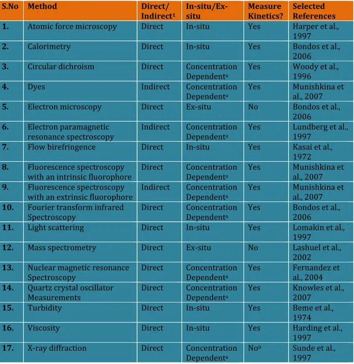
The working principle of AFM is that a small cantilever (typical length ~100 μm) with a sharp tip (1-10 nm end-of-curvature) scans a sample surface. As the tip encounters height differences or experiences changing tip-sample interaction forces, the cantilever bends (Figure

1.2). This deflection is detected and a feedback system moves the probe to keep the deflection at a

set value. In tapping mode AFM, the cantilever is oscillated, and feedback is usually done on either the tapping amplitude or frequency signal. In this way, an AFM maps the nanometer to micrometer scale topography and surface properties of the sample in a less invasive way.

Figure 1.2:Working principle of tapping mode atomic force microscopy. This simplified schematic gives an

overview of the main components of a beam deflection type AFM in amplitude-modulation tapping mode and explains the origins of the signals that will be referred to in the text. Comparing the amplitude signal with a pre-set pre-setpoint value yields the error signal. The feedback electronics uses this signal to adjust the voltage to the z-piezo, changing the height of the cantilever relative to the surface. Meanwhile, the phase detector compares the

phase of the amplitude signal with that of the tapping drive signal to yield the phase signal. [Reproduced from Ph.D. thesis Rajji 2008]

There are several ways to setup an AFM, but the scheme shown in Figure 1.2 is a commonly used one. There are several methods of cantilever deflection detection (optically: with quadrant detectors or interferometry, or mechanically using bimetals, to name a few), and there are several ways of controlling the motion of tip relative to sample (the piezo elements or other actuators can be in the piezo tube attached to the cantilever, or they can be in the sample stage), but the general working principle remains the same.

[1.2.1.1] Atomic force microscopy

The working principles of AFM are very simple. An atomically sharp tip is scanned over a surface with feedback mechanisms that enable the piezo-electric scanners to maintain the tip at a constant force (to obtain height information), or height (to obtain force information) above the sample surface. Tips are typically made up of Si3N4or Si, and extended down from the end of a cantilever.

The nanoscope AFM head employs an optical detection system in which the tip is attached to the underside of a reflective cantilever. A diode laser is focused onto the back of a reflective cantilever. As the tip scans the surface of the sample, moving up and down with the contour of the surface, the laser beam is deflected off the attached cantilever into a dual element photodiode. The photodetector measures the difference in light intensities between the upper and lower photodetectors, and then converts into voltage. Feedback from the photodiode difference signal, through software control from the computer, enables the tip to maintain either a constant force or constant height above the sample. In the constant force mode the piezo-electric transducer monitors real time height deviation. In the constant height mode the deflection force on the sample is recorded. The latter mode of operation requires calibration parameters of the scanning tip to be inserted in the sensitivity of the AFM head during force calibration of the microscope.

[1.2.1.2] Mode of operation

Contact mode

In contact mode atomic force microscopy (CM-AFM), the tip scans the sample in close contact with the surface, and the force between the tip and the surface kept constant during scanning by maintaining a constant deflection. This is the simplest mode used in the force microscope. The repulsive force on the tip is a mean value of 10ˉ⁹N. This force is set by pushing the cantilever

deflection of the cantilever is sensed and compared in a DC feedback amplifier to some desired value of deflection. The tip is effectively ‘dragged along’ the sample while the feedback loop keeps the interaction force constant by maintaining the deflection at a setpoint value. If the measured deflection is different from the desired value the feedback amplifier applies a voltage to the piezo to raise or lower the sample relative to the cantilever to restore the desired value of deflection. The voltage that the feedback amplifier applies to the piezo is a measure of the height of features on the sample surface. It is displayed as a function of the lateral position of the sample. This mode allows for very high lateral resolution on periodic samples with low corrugation, but is typically too damaging for protein aggregates.

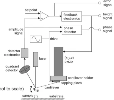
Non-contact mode

In non-contact mode atomic force microscopy (NCM-AFM), the tip of the cantilever does not come in contact with the sample surface. This is an important development in imaging that introduced a system for implementing the non-contact mode which is used in situations where tip contact might alter the sample in delicate ways. In this mode the tip floats 5-15 nm above the sample surface (Figure 1.3). Attractive Van der Waals forces acting between the tip and the sample are detected, and topographic images are constructed by scanning the tip above the surface. The attractive forces from the sample are substantially weaker than the forces used by contact mode. Therefore the tip must be given a small oscillation so that AC detection methods can be used to detect the small forces between the tip and the sample by measuring the change in amplitude, phase, or frequency of the oscillating cantilever in response to force gradients from the sample. For highest resolution, it is necessary to measure force gradients from Van der Waals forces which may extend only a nanometer from the sample surface. Measuring the tip to sample distance at each (x, y) data point allows the scanning software to construct a topographic image of the sample surface.

Figure 1.3:Non-contact mode atomic force microscope.

Figure 1.3 showing the scheme for dynamic mode of operation (both frequency and amplitude) in

non contact mode. In frequency modulation, information about the tip sample interaction can be observed by monitoring the change in oscillation frequency. In amplitude modulation, feedback signal for the image can be observed by the monitoring change in the oscillation amplitude or phase.

Non contact mode is good for the scanning of soft material in both liquid and air surface, whereas contact mode results into the degradation and damage of material by penetrating the surface in liquid medium.

Tapping mode

In tapping mode atomic force microscopy (TM-AFM), the cantilever oscillates at or near its resonance frequency. Feedback can be performed on the measured tapping amplitude or frequency [Garcia and Perez, 2002; Higgins et al., 2005], giving rise to the terms amplitude modulated AFM and frequency modulated AFM respectively. The intermittent tip-sample contact reduces lateral forces being exerted on the sample. The resonance frequency fres is typically in the 100 kHz range

in air, and in the 30 kHz range in liquid, and tapping amplitudes range from several nm in liquid to 100’s of nm in air. The minimum tapping amplitude that is necessary in air depends on the force needed to escape the thin water layer due to air humidity that is present on any surface exposed to air.

TM-AFM enables imaging of soft biological samples with minimal damage. This allows one to measure protein aggregate dimensions and material properties in a state as close as possible to the native state. In liquid, high frequency tapping may lead to apparent stiffening of soft biological samples, reducing tip induced damage even further on cells [Putman et al., 1994b].

TM-AFM mode is the most commonly used for imaging amyloid fibrils, and the amplitude of the tapping is one important factor that determines the extent of tip and sample wear. A second critical parameter is the setpoint ratio (s = Aset/Afree): the ratio of the tapping amplitude setpoint (to

which the feedback loop regulates the measured amplitude, see Figure 1.2), to the tapping amplitude when the cantilever is suspended free in air or water.

Because both attractive and repulsive forces act on the cantilever, and because they depend on the tip-sample separation in a nonlinear way, two stable oscillation states coexist in amplitude modulated AFM [reviewed in Garcia and Perez, 2002]. The equation of motion for the cantilever has two solutions: a high and a low amplitude branch. This means that a given setpoint tapping amplitude can be achieved at two distinct tip-sample separations. If the driving amplitude is large enough, both branches will merge into one, and only one stable solution to the equation of motion will exist [Garcia and Perez, 2002]. For low driving amplitudes however, the AFM operator should be aware that branch hopping (and related height artifacts) may occur. It is useful to qualitatively define tapping regimes. If s is lower than 30 %, we consider the tapping ‘hard’, if s > 70%, tapping is ‘soft’. In tapping mode experiments on TTR105−115 fibrils in air, [Mesquida et al., 2007] found that fibrils were not damaged by setpoint ratios between 10-80 %. This indicates the range of setpoint ratios used in amyloid research: the appropriateness of ‘hard’ or ‘soft’ tapping depends on the sample and the probe utilized.

[1.2.1.3] AFM as an imaging device

The atomic force microscope (AFM) is a representative example of instruments known as scanning probe microscope. Scanning probe microscope works by monitorning the value of a physical variable that depends on the distance between the surface to image and a specific probe. The topography of the surface is then reconstructed in three-dimensional detail. The prototype scanning probe microscope was the scanning tunneling microscope (STM), in which the probe is a microscopic electrode and the physical variable is the current between the electrode and a conductive surface on which the sample is placed. The tunneling current, varying exponentially and very steeply with distance, is a sensible probe of surface topography. AFM instead works using

probe displacement as the variable, being similar conceptually to a miniature phonograph. The probe itself is a solid, sharp microscopic tip located at the end of a flexible cantilever.

The tip and the surface are put in contact or close proximity, and the cantilever deflection due to the tip sample interactions is the variable being monitored. The cantilever, normally, can be modeled as a simple Hookean spring and therefore its response is linear with applied force. In most cases, cantilever deflection is in turn probed and amplified by a laser beam that reflects on the cantilever very end, forming a so-called optical lever system. The laser beam reflected by the tip hits a photodiode, which records the displacement of the laser beam from a reference point. The system in this way achieves a resolution of the order of the nanometer.

A piezoelectric scanner is usually used to move the sample (or the tip) in three dimensions, allowing the tip to scan various portions of the sample. Piezoelectric scanners allow AFMs to reach 1 nm of lateral resolution. Atomic resolution has been reached vertically for hard materials in vacuum conditions. On the other hand, AFM can easily be applied to biological samples because it requires little or no sample preparation and works readily in physiological conditions (liquid buffer, room temperature etc.). Live eukaryotic cells can be extensively analyzed with the AFM [Mathur et al., 2001].

[1.2.1.4] Imaging conditions

AFM on biomaterials can be performed in air or in a liquid, such as an aqueous pH-buffering solution.

Imaging in air

The main advantages of imaging in air are, (i) that sample preparation is easier, sample no need to put in liquid, and (ii) the sample can be used for long time after preparation without degradation. A disadvantage of AFM in air compared to in liquid is that a tapping amplitude in the order of 100 nm is required (with associated high tapping force) to overcome the strong capillary force that is due to a thin water layer that tends to form on the substrate surface.

Imaging in liquid

One undeniable reason for imaging in liquid is that in liquid environment physiological conditions resembles much more close to the proteins and other biological systems. Also, in an aqueous environment it is possible to study biomolecular interactions.

In the case of amyloid fibrils, a disadvantage of imaging in liquid is their higher fragility in liquid than in air. Also, it is sometimes hard to bind the sample to the substrate (although that seems to be more of a problem for DNA than for protein aggregates). Another disadvantage is that the samples cannot be kept for the next use, since the evaporation of the water droplet leads to buffer salt deposition, while continued immersion in a large quantity of buffer would presumably lead to desorption of the aggregates. A major application for AFM imaging in buffer is that aggregations can be monitored in real-time through in situ imaging: when the buffer contains monomers of the protein of interest and the buffer conditions are right, surface templated aggregation may occur [Hoyer et al., 2004]. Also, the directionality of fibril growth becomes accessible [Blackley et al., 2000; Goldsbury et al., 1999; Zhu et al., 2002].

[1.2.1.5] Choice of probe and substrate

An AFM probe consists of a cantilever with a tip, and its properties are critical to the results of the imaging of biomolecular samples. The lateral resolution of AFM images depends on the sharpness of the tip that is used, and the cantilever stiffness and resonance frequency determine the force exerted on the sample, and any resulting damage.

The substrate used for imaging of amyloid fibrils is a relevant factor in in-situ aggregation studies: the fibrils may form a pattern based on the atomic structure of the substrate [Yang et al., 2002]. The properties of the surface on which the sample is deposited also influence the kinetics and morphology of amyloid fibril formation. In an in-situ TM-AFM study in liquid, the morphology of Aβ aggregates was different on hydrophilic mica than on hydrophobic graphite: on mica, particulate aggregates formed, whereas on graphite, linear assemblies similar to protofilaments formed [Kowalewski and Holtzman, 1999]. This dependence of fibril morphology on substrate hydrophobicity implies that fibril formation may be expedited on interfaces between aqueous solutions and lipid surfaces, as would occur at cellular membranes and lipoprotein particles in a living cell. Aβ1−42 early aggregates deposit with a higher yield on hydrophilic mica than on hydrophobic graphite, and the opposite is true for mature fibrils [Arimon et al., 2005]. Finally, hydrophobic surface favor the formation of surface nanobubbles [Yang et al., 2007], which is undesirable when imaging proteins. For AFM imaging of protein fibrils, freshly cleaved mica appears to be the most convenient substrate.

[1.2.1.6] Force spectroscopy

In addition to these topographic measurements, the AFM can also provide much more information about the molecular motion behavior and fluctuation of the single molecule (both biological and non-biological) at nano-scale. The AFM can also record the amount of force felt by the cantilever as the probe tip is brought close to and even indented into a sample surface and then pulled away. This technique can be used to measure the long range attractive or repulsive forces between the probe tip and the sample surface, elucidating local chemical and mechanical properties like adhesion and elasticity, and even thickness of adsorbed molecular layers or bond rupture lengths.

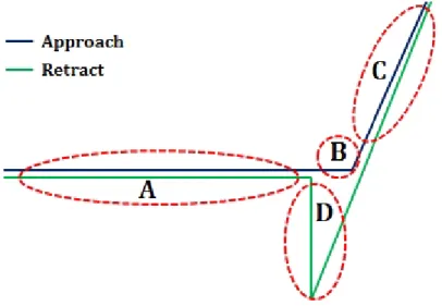
Force curves (force-vs-distance curve) typically show the deflection of the free end of the AFM cantilever as the fixed end of the cantilever is brought vertically towards and then away from the sample surface. Experimentally, this is done by applying a triangle-wave voltage pattern to the electrodes for the z-axis scanner. This causes the scanner to expand and then contract in the vertical direction, generating relative motion between the cantilever and sample. The deflection of the free end of the cantilever is measured and plotted at many points as the z-axis scanner extends the cantilever towards the surface and then retracts it again. By controlling the amplitude and frequency of the triangle-wave voltage pattern, the researcher can vary the distance and speed that the AFM cantilever tip travels during the force measurement.

Similar measurements can be made with oscillating probe systems like Tapping Mode and non-contact AFM. This sort of work is just beginning for oscillating probe systems, but measurements of cantilever amplitude and/or phase versus separation can provide more information about the details of magnetic and electric fields over surfaces and also provide information about viscoelastic properties of sample surfaces.

[1.2.1.7] Anatomy of a force curve

A: In this region cantilever does not touch the surface, if the cantilever feels a long-range attractive

(or repulsive) force it will deflect downwards (or upwards) before making contact with the surface.

B: As the probe tip is brought very close to the surface, it may jump into contact if it feels sufficient

Figure 1.4: Atypical AFM force curve.

C: Once the tip is in contact with the surface, cantilever deflection will increase as the fixed end of

the cantilever is brought closer to the sample. If the cantilever is sufficiently stiff, the probe tip may indent into the surface at this point. In this case, the slope or shape of the contact part of the force curve can provide information about the elasticity of the sample surface.

D: After loading the cantilever to a desired force value, the process is reversed. As the cantilever is

withdrawn, adhesion or bonds formed during contact with the surface may cause the cantilever to adhere to the sample some distance past the initial contact point on the approach curve (B).

A key measurement of the AFM force curve is the point at which the adhesion is broken and the cantilever comes free from the surface. This can be used to measure the rupture force required to break the bond or adhesion.

[1.2.1.8] AFM calibration

The cantilever elastic constant needs to be measured for each experiment: this is due to unavoidable inhomogeneities in the batches of commercial cantilevers. This is usually done day to day by the “thermal tune” method that is by measuring the thermal oscillation spectrum of the free cantilever (not in touch with any surface) and using the equipartition theorem to obtain the actual elastic constant. The cantilever is here treated as a simple oscillator and the Brownian motion of the main fundamental oscillation mode of the cantilever gives the elastic constant by the simple formula:

where the Boltzmann constant, T is is temperature and is the square mean cantilever deflection.

This latter variable is found by fitting the power spectrum of the cantilever thermal noise, with the advantage of avoiding interference from both non-thermal oscillation at other discrete frequencies and white noise.

In practice, it must be noticed that today more complex, empirical equations are used, to correct significant deviations from the ideal oscillator behaviour of the cantilever. The typical error is ±20% [Hutter et al., 1993; Florin et al., 1995]. The other essential parameter to be known is the optical lever sensitivity, i.e. the ratio between cantilever deflection and the photodiod output voltage difference. This depends from the optical properties of the cantilever, the medium (air or water), the eventually present fluid cell etc. and also needs to be measured for each cantilever. This is usually done by pressing the cantilever on a hard surface (i.e. glass or mica) at high forces: assuming that no substrate deformations happen, the cantilever deflection must be theorically equal to the piezo movement and the ratio can be calculated. When this is done, the sample can be put in place under the tip. There are a number of free parameters that the experimenter must decide before starting the experiment (most of them can also be changed during operation): the speed, the length range, the maximum force acting on contact on the surface, the scan rate (number of points recorded per second) are usually the most important.

[1.2.1.9] AFM vs other imaging technique

AFM vs STM

It is an interesting to compare AFM and its precursor Scanning Tunneling Microscope. In some cases, the resolution of STM is better than AFM because of the exponential dependence of the tunneling current on distance. The force-distance dependence in AFM is much more complex when characteristics such as tip shape and contact force are considered. STM is generally applicable only to conducting samples while AFM is applied to both conductors and insulators. In terms of versatility, needless to say, the AFM wins. Furthermore, the AFM offers the advantage that the writing voltage and tip-to-substrate spacing can be controlled independently, whereas with STM the two parameters are integrally linked.

AFM vs SEM

Compared with Scanning Electron Microscope, AFM provides extraordinary topographic contrast direct height measurements and unobscured views of surface features (no coating is necessary).

AFM vs TEM

Compared with Transmission Electron Microscopes, three dimensional AFM images are obtained without expensive sample preparation and yield far more complete information than the two dimensional profiles available from cross-sectioned samples.

AFM vs Optical microscope

Compared with Optical Interferometric Microscope (optical profiles), the AFM provides unambiguous measurement of step heights, independent of reflectivity differences between materials.

[1.2.2] Fluorescence polarization

Fluorescence Polarization (FP) was first described by Perrin in 1926. When a small fluorescent molecule is excited with plane-polarized light, the emitted light is largely depolarized because molecules tumble rapidly in solution during their fluorescence lifetime (the time between excitation and emission). It is a powerful tool to study molecular interactions (protein-protein, protein-DNA and protein-ligands) by monitoring changes in the apparent size of fluorescently-labeled or inherently fluorescent molecules.

Principle behind fluorescence polarization

When a fluorescent molecule is excited with plane polarized light, light is emitted in the same polarized plane, provided that the molecule remains stationary throughout the excited state (which has duration of 4 nanoseconds for fluorescein). If the molecule rotates and tumbles out of this plane during the excited state, light is emitted in a different plane from the excitation light. If vertically polarized light is exciting the fluorophore, the intensity of the emitted light can be monitored in vertical and horizontal planes (degree of movement of emission intensity from vertical to horizontal plane is related to the mobility of the fluorescently labeled molecule (see Figure 1.4)). If a molecule is very large, little movement occurs during excitation and the emitted light remains highly polarized. If a molecule is small, rotation and tumbling is faster and the emitted light is depolarized relative to the excitation plane.

Figure 1.5:Scheme showing polarization of plane polarized light by fluorescent molecule in fluorescent polarization experiment.

Polarization is defined as a function of the observed parallel ( ) and perpendicular intensities ( ): (2.2) If the emission is completely polarized in the parallel direction, i.e., the electric vector of the exciting light is totally maintained, then:

(2.3) If the emitted light is totally polarized in the perpendicular direction then:

(2.4) The limits of polarization are thus +1 to -1

Another term frequently used in the context of polarization is anisotropy (usually designated as either A or r) which is defined as:

(2.5) By analogy to polarization, the limits of anisotropy are +1 to -0.5

(2.6) Or (2.7) For example P r 0.50 0.40 0.30 0.22 0.10 0.069

Clearly, the information content in the polarization function and the anisotropy function is identical and the use of one term or the other is dictated by practical consideration.

Small molecules rotate quickly during the excited state, and upon emission, have low polarization values. Large molecules, caused by binding of a second molecule, rotate little during the excited state, and therefore have high polarization values.

Dependence of fluorescence polarization on molecular mobility

Interpretation of the dependence of the fluorescence polarization on molecular mobility is usually based on a model derived in 1926 from the physical theory of Brownian motion by Perrin:

(2.8) Where is the fundamental polarization of the dye (for fluorescein, rhodamine and BODIPY dyes,

is close to the theoretical maximum of 0.5), r is the excited-state lifetime of the dye and is the rotational correlation time of the dye or dye conjugate. These relationships can be expressed in terms of fluorescence anisotropy in an equivalent and mathematically simpler manner. For a hydrodynamic sphere, can be estimated as follows:

Where η = solvent viscosity, T = temperature, R = gas constant and V = molecular volume of the fluorescent dye or dye conjugate. In turn, V can be estimated from the molecular weight of the dye or dye conjugate with appropriate adjustments for hydration.

Polarizer

The most common polarizers used today are (i) dichroic devices, which operate by effectively absorbing one plane of polarization (e.g. Polaroid type-H sheets based on stretched polyvinyl alcohol impregnated with iodine) and (ii) double refracting calcite (CaCO3) crystal polarizers which differentially disperse the two planes of polarization (examples of this class of polarizers are Nicol polarizers, Wollaston prisms and type polarizers such as the Foucault, Glan-Thompson and Glan-Taylor polarizers).

[1.3] α-Synuclein

[1.3.1] Historical overview

The name ‘Synuclein’ was first derived from the protein that was found in both synapses and in the

nuclear envelope [Maroteaux et al., 1988]. The 143-amino acid (aa) long neurone-specific protein

was isolated from the electric organ of the fish Torpedo californica by expression screening was called synuclein. Independently, NACP, the 140-aa non-Aβ component of AD amyloid precursor [Ueda et al., 1993], and synelfin [George et al., 1995] were cloned in human and in the zebra finch, respectively. They were found to be orthologs of torpedo fish synuclein and rat brain synuclein [Campion et al., 1995; Maroteaux et al., 1991; Jakes et al., 1994]. When Jakes et al. cloned β-synuclein as a second member of the human β-synuclein family, they termed the initially isolated family members ‘α-synuclein.’ All α-synucleins were shown to be extremely well conserved among distantly related species [George et al., 1995; Maroteaux et al., 1991; Jakes et al., 1994]. α-Synuclein was not found in the nucleus in several subsequent studies. It appears therefore to be a purely presynaptic protein [Jakes et al., 1994; Iwai et al., 1995].

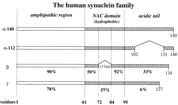
[1.3.2] The Synuclein family

Three members of the human synuclein family have been identified: α-, β-, and γ-synuclein (see

Figure 1.6). The genes are located on chromosome 4q21 [Shibasaki et al., 1995; Spillantini et al.,

1995; campion et al., 1995 and Chen et al., 1995], 5q35 [Spillantini et al., 1995], and 10q23 [Lavedan et al., 1998], respectively.