Contents
0 Introduction 1
1 Interpolation 4
1.1 General problem of finite interpolation . . . 4
1.2 Systems possessing the ”interpolation property” . . . 6
1.3 Representation of the solution of the interpolation problem in linear spaces 12 1.4 Representation of the remainder for polynomial interpolation . . . 19
1.5 Peano’s Theorem and its consequence . . . 21
1.6 General remainder theorem for interpolation in linear spaces . . . 28
2 Appell polynomials 29 2.1 Introduction . . . 29
2.2 A determinantal definition . . . 32
2.3 General properties of Appell polynomials . . . 40
2.4 Fourier series expansion of Appell polynomials . . . 50
2.5 Examples . . . 53
2.5.1 Bernoulli polynomials . . . 53
2.5.2 Generalized Bernoulli polynomials . . . 55
2.5.3 Hermite normalized polynomials . . . 55
2.5.4 Generalized Hermite polynomials . . . 56
2.5.5 Generalized Laguerre polynomials . . . 56
2.5.6 Euler polynomials . . . 56
2.5.7 Generalized Euler polynomials . . . 59
2.6 Numerical examples . . . 59
2.6.1 Bernoulli-Jacobi/Tchebichev polynomials . . . 60
2.6.2 Generalized Laguerre polynomials . . . 61
2.6.3 Generalized Euler polynomials . . . 62
3 Appell interpolation problem 63 3.1 The Appell interpolation problem . . . 63
3.2 The remainder . . . 68
3.3.1 The Taylor interpolation polynomial . . . 71
3.3.2 The Bernoulli interpolation polynomial . . . 74
3.3.3 The Bernoulli generalized interpolation polynomial . . . 76
3.3.4 The Euler interpolation polynomial . . . 77
3.3.5 The Euler generalized interpolation polynomial . . . 79
3.3.6 The Hermite normalized interpolation polynomial . . . 81
3.3.7 The Hermite generalized interpolation polynomial . . . 82
3.3.8 The Laguerre generalized interpolation polynomial . . . 83
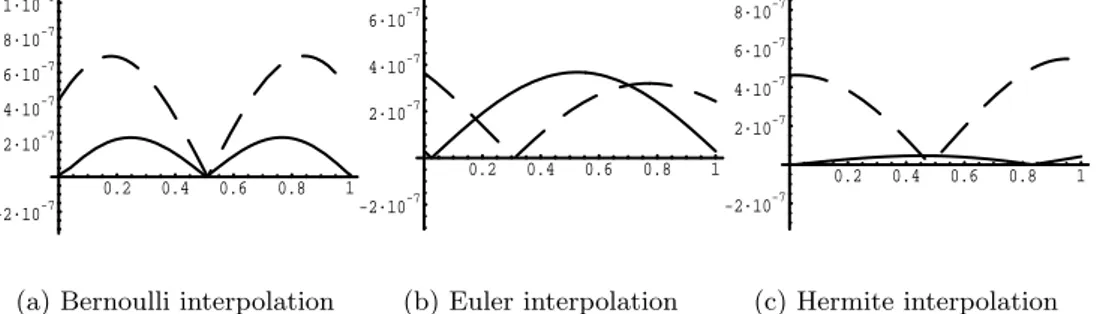
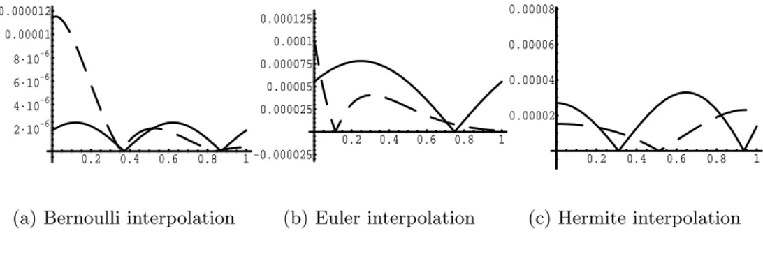
3.4 Numerical examples . . . 83
4 Bernoulli, Lidstone and Fourier series for real entire functions of expo-nential type 87 4.1 Introduction . . . 87
4.2 Preliminary and known results . . . 88
4.3 Equivalence of Bernoulli and Lidstone series with Fourier series . . . 90
5 A Birkhoff interpolation problem 95 5.1 Introduction . . . 95
5.2 The solution . . . 96
5.3 The remainder . . . 101
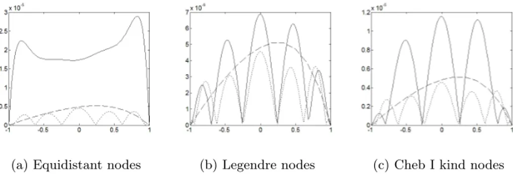
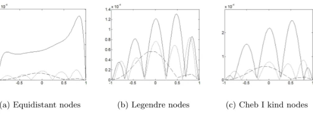
5.4 Examples . . . 104
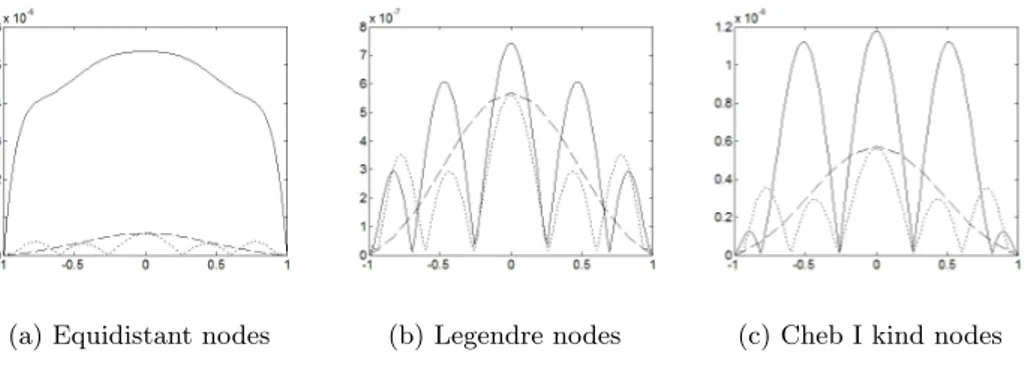
5.4.1 Equidistant nodes . . . 105
5.4.2 Chebyshev of second kind nodes . . . 106
5.5 Quadrature formulae . . . 107
5.5.1 Examples . . . 110
6 A new collocation method for a BVP 112 6.1 The method . . . 112
6.2 Global error . . . 114
6.3 The numerical algorithm and numerical comparison . . . 115 A Mathematica code for computation of polynomials pn,i(x) 120 B Computation of coefficients An,i for equidistant nodes 122 C Computation of coefficients An,i for Chebyshev of second kind nodes 123
Ringraziamenti 125
Chapter 0
Introduction
The study of real phenomenons leads, very often, to the analysis of functions not easily usable, that because of their complicated analytic expressions which are too complex to evaluate efficiently or because of the functions studied are known only in a number of data points. From that the necessity of approximate a function with a simpler mathematical expression taking account of its known values and minimizing the remainder. Interpolation is a method of approximating a given function using data that are available at a distribution of data points. The data can be consist, for example, of the function values or some of its derivatives. The general approach is to construct an interpolating function, the interpolant, which fits the available data perfectly. Among the different classes of functions in which find the interpolants, the polynomial one is the most studied because of its known characteris-tics. In the following, at first we deal with the problem from a general point of view, that is in an arbitrary linear space of finite dimension, then we focus our study on two different polynomial interpolation problems of which we examine some applications. In Chapter 1 we
consider interpolation, remainder theory, convergence theorems for interpolatory processes and some classic problems of finite interpolation. We also present a number of basic defini-tions and elementary properties that will be of use in the later chapters. In Chapter 2 we introduce the sequences of Appell polynomials for which we provides an algebraic approach with the aim of giving a unifying theory for all classis of Appell polynomials and a their very natural generalization. We establish the equivalence of the new approach with the previous characterizations through a circular theorem. Moreover, we give general proper-ties of Appell polynomials by employing basic tools of linear algebra and we consider their expansion in Fourier series. We also propose an efficient and stable Gaussian algorithm for the computation of the coefficients for particular sequences of Appell polynomials and consider classic examples, in particular Bernoulli, Euler, normalized Hermite and Laguerre polynomials and their possible generalizations not studied in the literature so far. Finally, the proposed algebraic approach allows the solution, expressed by a determinantal form us-ing a basis of Appell polynomials, of a remarkable new general linear interpolation problem. In Chapter 3 we examine this interpolation problem related to the Appell polynomials and we provide an explicit solution of it and a study of the remainder. Moreover, we consider classic examples, in particular Taylor, Bernoulli, Euler, normalized Hermite and Laguerre polynomials and their possible generalizations. We also present certain numerical examples to test the method proposed. In Chapter 4 we consider series related to particular inter-polation problems, as Bernoulli and Lidstone, and we prove that, for real entire functions of exponential type, these expansions coincide with the known Fourier series. In Chapter 5 we introduce a new interpolation problem of Birkhoff kind. Birkhoff, or lacunary,
in-terpolation appears whenever observation gives scattered or irregular information about a function and its derivatives. Lacunary interpolation differs radically from the more familiar of Lagrange and Hermite interpolation for which the interpolation polynomial always exists, is unique, and can be given by an explicit formula. In particular our study deals with an interpolation problem in which the data are the function values at boundary points of a given interval [a, b] and its second derivative at n − 1 internal points of the interval [a, b]. We provide an explicit solution of the interpolation problem considered and an estimation error. Moreover, we study the convergence of the method and we give the examples of equidistant interpolation points and Chebyshev points. Finally, as application of this inter-polation problem, we consider a new class of interpolatory type quadrature formulae, called extended Gauss-Birkhoff quadratures with respect to a weight function w.
In Chapter 6 we examine a boundary value problem related to the interpolatory problem proposed in the previous chapter. We provide a general procedure to determine collocation methods for this problem and we give an a-priori estimation error. We also propose a numerical algorithm for the calculation and, finally, present certain numerical examples to compare the method proposed with the Matlab build-in function bvp4c.
Chapter 1
Interpolation
In this chapter we present a number of basic definitions, main theorems and ele-mentary properties from interpolation theory that will be of use in the later chapters.
1.1
General problem of finite interpolation
The general problem of finite interpolation ([21]) is the following:
Let X be a linear space of dimension n and let L1, L2, ..., Ln be n given linear functionals defined on X. For a given set of values ω1, ω2, ..., ωn, find, if it exists, an
element x ∈ X such that
Li(x) = ωi, i = 0, ..., n. (1.1)
For the solution we consider the following
Lemma 1 Let X have dimension n. If x1, x2, ..., xnare independent in X and L1, L2, ..., Ln
are independent in the dual space X∗ then
Conversely, if either x1, x2, ..., xn or L1, L2, ..., Ln are independent and (1.2) holds then the
other set is also independent.
Proof. Suppose that |Li(xj)| = 0. Then also |Lj(xi)| = 0. The linear system a1L1(x1) + a2L2(x1) + ... + anLn(x1) = 0 .. . ... a1L1(xn) + a2L2(xn) + ... + anLn(xn) = 0 would have a nontrivial solution a1, a2, ..., an.
The property of linearity of functional Li implies that
(a1L1+ a2L2+ ... + anLn)(xi) = 0, i = 1, ...., n. Since x1, x2, ..., xn form a basis for X,
(a1L1+ a2L2+ ... + anLn)(x) = 0, x ∈ X, and hence a1L1+ a2L2+ ... + anLn= 0.
Therefore, L1, L2, ..., Ln are dependents contrary to our assumption. To show the converse, we may trace the argument backwards.
Theorem 2 Let a linear space X have dimension n and let L1, L2, ..., Ln be n elements of
X∗. The interpolation problem (1.1) possesses a solution for arbitrary values ω
1, ω2, ..., ωn
if and only if the Li are independent in X∗. The solution will be unique.
Proof. Let x1, x2, ..., xn be a basis for X. If L1, L2, ..., Ln are independent, then, by lemma 1,
|Li(xj)| 6= 0. Hence the system
Li(a1x1+ a2x2+ ... + anxn) = ωi, i = 1, 2, ...n or
a1Li(x1) + a2Li(x2) + ... + anLi(xn) = ωi (1.3) possesses a solution a1, a2, ..., an and the element
a1x1+ a2x2+ ... + anxn solves the interpolation problem (1.1).
Conversely, if the problem has a solution for arbitrary ωi, then the system (1.3) has a solution for arbitrary ωi. By a known theorem of linear algebra, this implies that
|Li(xj)| 6= 0
and hence by 1, the Li are independent.
The determinant |Li(xj)| is a generalized Gram determinant and its nonvanishing is synonymous with the possibility of solution of the interpolation problem.
We may speak of independent systems of functionals as having the ”interpolation property”.
1.2
Systems possessing the ”interpolation property”
We study, now, some spaces and functionals for which the interpolation problem can be solved.
Example 3 (Interpolation at discrete points)
X = Pn. L0(f ) = f (z0), L1(f ) = f (z1), ..., Ln(f ) = f (zn).
We assume that zi6= zj, i 6= j.
Example 4 (Taylor Interpolation)
X = Pn. L0(f ) = f (z0), L1(f ) = f0(z0), ..., Ln(f ) = f(n)(z0).
Example 5 (Abel-Gontscharoff Interpolation)
X = Pn. L0(f ) = f (z0), L1(f ) = f0(z1), ..., Ln(f ) = f(n)(zn). Example 6 (Lidstone Interpolation)
X = P2n+1. L1(f ) = f (z0), L2(f ) = f (z1)
L3(f ) = f00(z0), L4(f ) = f00(z1)
..
. ...
L2n+1(f ) = f(2n)(z0), L2n+2(f ) = f(2n)(z1), (z0 6= z1).
Example 7 (Lidstone of Second Type Interpolation)
X = P2n+1. L1(f ) = f0(z0), L2(f ) = f0(z1)
L3(f ) = f000(z0), L4(f ) = f000(z1)
..
. ...
Example 8 (Simple Hermite or Osculatory Interpolation) X = P2n−1. L1(f ) = f (z1), L2(f ) = f0(z1) L3(f ) = f (z2), L4(f ) = f0(z2) .. . ... L2n−1(f ) = f (zn), L2n(f ) = f0(zn), (zi 6= zj, i 6= j). Example 9 (Full Hermite Interpolation)
X = Pn. To avoid indexing difficulties, we list the functional information employed
without using the symbol L. f (z0), f0(z 0), ..., f(m0)(z0) f (z1), f0(z1), ..., f(m1)(z1) .. . f (zn), f0(z n), ..., f(mn)(zn) (zi6= zj, N = m0+ m1+ ... + mn+ n). Example 10 (Generalized Taylor Interpolation)
X consists of the linear combination of the n + 1 linearly independent functions
ϕ0(z), ϕ1(z), ..., ϕn(z)
that are analytic at z0.
L0(f ) = f (z0), L1(f ) = f0(z0), ...., Ln(f ) = f(n)(z0). ¯ ¯ ¯ϕ(j)i (z0) ¯ ¯ ¯ 6= 0.
A linear combination of 1, cos x, ..., cos nx, sin x, ..., sin nx is known as a trigono-metric polynomial of degree ≤ n. The corresponding linear space will be designate by Tn. It
has dimension 2n + 1.
X = Tn. L0(f ) = f (x0), L1(f ) = f0(x0), ..., L2n(f ) = f(2n)(x0),
−π ≤ x0< x1 < . . . < x2n< π.
Example 12 (Fourier Series)
X = Tn. L2k(f ) = Rπ −πf (x) cos kxdx, k = 0, 1, ..., n. L2k−1(f ) = Rπ −πf (x) sin kxdx, k = 1, ..., n.
Before demonstrating that these functionals are independent over the respective spaces, a few remarks are in order. Ex. 3 is, of course, Theorem 2. Exs. 3, 4, 8 are special cases of Ex. 9 . Ex. 4, is a special case of Ex. 10 if we select ϕk(z) = zk.
To show that the interpolation problem formed from these examples has a solution it suffices to show that det(Li(xj)) does not vanish, or to apply the following
Theorem 13 (Alternative Theorem) Consider the system of n linear equations in n
unknowns x1, x2, ..., xn
n X J=1
aijxj = bi (i = 1, 2, ...n) (1.4)
the homogeneous system
n X J=1
aijxj = 0 (i = 1, 2, ...n) (1.5)
possesses a non-trivial solution if and only if |A| = |aij| = 0. If for a fixed A = (aij) there
are solutions to the non-homogeneous system (1.4) for every selection of the quantities bi,
Solution 14 (Example 4) We show that if p ∈ PN and satisfies p(z0), p0(z0), ..., p(m0)(z0) = 0 p(z1), p0(z 1), ..., p(m1)(z1) = 0 .. . p(zn), p0(zn), ..., p(mn)(zn) = 0 (1.6)
where N = m0+ m1+ ... + mn+ n, then p must vanish identically. By the Factorization
Theorem, if p satisfies all conditions of (1.6) with the exception of the last, i.e., p(mn)(z
n) = 0, then we must have
p(z) = A(z)(z − z0)m0+1(z − z1)m1+1...(z − zn−1)mn−1+1(z − zn)mn,
A(z) = polinomial.
By examining the degree of this product, it appears that A = constant. Since, moreover, p(mn)(z
n) = A(mn)!(zn− z0)m0+1(zn− z1)m1+1...(zn− zn−1)mn−1+1= 0
and zi 6= zj, i 6= j, we have A = 0 and therefore p ≡ 0. The homogeneous interpolation
problem has the zero solution only and hence the nonhomogeneous problem possesses a unique solution.
Solution 15 (Example 5) The generalized Gram determinant is ¯ ¯ ¯ ¯ ¯ ¯ ¯ ¯ ¯ ¯ ¯ ¯ ¯ ¯ ¯ ¯ ¯ ¯ ¯ ¯ 1 z0 z20 · · · z0n 0 1 2z1 · · · nz1n−1 0 0 2 · · · n(n − 1)zn−22 .. . ... 0 0 0 · · · n! ¯ ¯ ¯ ¯ ¯ ¯ ¯ ¯ ¯ ¯ ¯ ¯ ¯ ¯ ¯ ¯ ¯ ¯ ¯ ¯ = 1!2! · · · n! 6= 0.
Solution 16 (Example 6) Let p ∈ P2n+1. If p(2j)(z0) = 0 for j = 0, 1, ..., n, then
p(z) = a1(z − z0) + a3(z − z0)3+ ... + a2n+1(z − z0)2n+1.
If now, p(2n)(z
1) = 0 then a2n+1 = 0 e p(2j)(z1) = 0, j = n − 1, n − 2, ...0 implies, by
recurrence, that the remaining coefficients are 0. The homogeneous interpolation problem has the zero solution only and hence the nonhomogeneous problem has a solution and it is unique.
Solution 17 (Example 7) With the same techniques used for the Ex. 6 we can prove that
the homogeneous interpolation problem has the zero solution only and hence the nonhomo-geneous problem has a solution and it is unique.
Solution 18 (Example 10) No proof is required, for condition (1.2) has been built into
the hypothesis. In this example the crucial determinant reduces to the Wronskian of the functions φ0, ..., φn and we postulate that it does not vanish at z0.
Solution 19 (Example 11) The generalized Gram determinant is
G = ¯ ¯ ¯ ¯ ¯ ¯ ¯ ¯ ¯ ¯ ¯ ¯ ¯ ¯ ¯ ¯
1 cos x0 sin x0 cos 2x0 sin 2x0 · · · cos nx0 sin nx0
1 cos x1 sin x1 cos 2x1 sin 2x1 · · · cos nx1 sin nx1
1 cos x2n sin x2n cos 2x2n sin 2x2n · · · cos nx2n sin nx2n
¯ ¯ ¯ ¯ ¯ ¯ ¯ ¯ ¯ ¯ ¯ ¯ ¯ ¯ ¯ ¯ .
To evaluate G we reduce its element to complex form. Multiply the 3rd, 5th,... columns by ı and add them respectively to the 2nd, 4th,... columns. We obtain
G = ¯ ¯ ¯ ¯ 1 eıxjsin x j e2ıxjsin 2xj · · · enıxjsin nxj ¯ ¯ ¯ ¯ .
Multiply the 3rd, 5th,... columns by −2ı and to them add the 2nd, 4th,... columns respec-tively: (−2ı)(n)G = ¯ ¯ ¯ ¯ 1 eıxj e−ıxj e2ıxj e−2ıxj · · · enıxj e−nıxj ¯ ¯ ¯ ¯ .
Interchange the columns:
(−1)n(n+1)(−2ı)(n)G = ¯ ¯ ¯ ¯ e−nıxj e−(n−1)ıxj · · · 1 · · · e(n−1)ıxj enıxj ¯ ¯ ¯ ¯ .
Multiply the j − th row by enıxj, j = 0, ...., 2n:
enı(x0+x1+···+x2n)(−1)n(n+1)(−2ı)(n)G = ¯ ¯ ¯ ¯ 1 eıxj e2ıxj · · · enıxj ¯ ¯ ¯ ¯ .
The determinant in the last line is a Vandermonde. Hence, enı(x0+x1+···+x2n)(−1)n(n+1)(−2ı)(n)G =
2n
Y j>k
(eıxj− eıxk).
In view of the conditions on the xj, eıxj 6= eıxk, j 6= k and so G 6= 0.
Solution 20 (Example 12) In view of the orthogonality of the sines and cosines, the
crucial determinant has positive quantities on the main diagonal and 0’s elsewhere and hence does not vanish.
1.3
Representation of the solution of the interpolation
prob-lem in linear spaces
Theorem 21 Let X be a linear space of dimension n. Let L1, L2, ...Ln be n
indepen-dent functional in X∗. Then, there are determined uniquely n independent elements of X,
x∗
1, x∗2, ..., x∗n, such that
where with δij we denoted the Kronecker symbol δij = 0 se i 6= j 1 se i = j .
For any x ∈ X we have
x =
n X i=1
Li(x)x∗i. (1.8)
For every choice of ω1, ω2, ..., ωn, the element x =
n X i=1
ωix∗i (1.9)
is the unique solution of the interpolation problem
Li(x) = ωi, i = 1, 2, ..., n. (1.10)
Proof. Let x1, x2, ..., xn be a basis for X. By Lemma 1, |Li(xj)| 6= 0. If we set
x∗
i = aj1x1 + . . . + ajnxn, j = 1, ..., n, then this determinant condition guarantees that the system (1.7) can be solved for aji to produce a set of elements x∗
1, x∗2, ..., x∗n ∈ X. By Theorem 2 the solution to the interpolation problem (1.7) is unique, for each j, and by Lemma 1 the x∗
i are independent. To prove the (1.8) denote
y =
n X i=1
Li(x)x∗i
and for the property of linearity of functionals Lj we have
Lj(y) = n X
i=1
Li(x)Lj(x∗i).
Hence, by (1.7), Lj(y) = Lj(x), j = 1, 2, ..., n. Again, since the interpolation with n condition Liis unique, y=x and this establishes (1.8). Equation (1.9) is established similarly.
We will say that the elements x∗
i ∈ X and the functionals Li are biorthonormal if they satisfy the (1.7). For a given set of independent functional, we can always find a related biorthonormal set of polynomials.
The solution of the interpolation problem (1.10) can be given in determinantal form.
Theorem 22 Let the hypotheses of Theorem 21 hold and let x1, x2, ..., xn be a basis for X.
If ω1, ω2, ..., ωn are arbitrary numbers then the element
x = −1 G ¯ ¯ ¯ ¯ ¯ ¯ ¯ ¯ ¯ ¯ ¯ ¯ ¯ ¯ ¯ ¯ ¯ ¯ ¯ ¯ 0 x1 x2 · · · xn ω1 L1(x1) L1(x2) · · · L1(xn) .. . ... .. . ... ωn Ln(x1) Ln(x2) · · · Ln(xn) ¯ ¯ ¯ ¯ ¯ ¯ ¯ ¯ ¯ ¯ ¯ ¯ ¯ ¯ ¯ ¯ ¯ ¯ ¯ ¯ , (1.11) where G = |Li(xj)|, satisfies Li(x) = ωi, i = 1, 2, ..., n.
Proof. It is clear that x is a linear combination of x1, x2, ..., xn and hence is in
X. Furthermore, we have Li(x) = −G1 ¯ ¯ ¯ ¯ ¯ ¯ ¯ ¯ ¯ ¯ ¯ ¯ ¯ ¯ ¯ ¯ ¯ ¯ ¯ ¯ ¯ ¯ ¯ ¯ ¯ 0 Li(x1) Li(x2) · · · Li(xn) ω1 L1(x1) L1(x2) · · · L1(xn) .. . ... ωi Li(x1) Li(x2) · · · Li(xn) .. . ... ωn Ln(x1) Ln(x2) · · · Ln(xn) ¯ ¯ ¯ ¯ ¯ ¯ ¯ ¯ ¯ ¯ ¯ ¯ ¯ ¯ ¯ ¯ ¯ ¯ ¯ ¯ ¯ ¯ ¯ ¯ ¯ . (1.12)
Expand this determinant by minors of the 1st column. The minor of each nonzero element, with the exception of ωi, is zero, for it contains two identical rows. The cofactor of ωi is
−G. Hence, Li(x) = ωi, i = 1, 2, ..., n.
Example 23 (Taylor Interpolation)
The polynomials zn
n!, n = 0, 1, ..., and the functionals Ln(f ) = f(n)(0), n = 0, 1, ..., are biorthonormal, for Li(
zj
j!) = δij.
Example 24 (Osculatory Interpolation)
Set ω(z) = (z − z1)(z − z2) · · · (z − zn), lk(z) = (z − zω(z) k)ω0(zk). The polynomials · 1 −ω00(zk) ω0(zk)(z − zk) ¸ l2
k(z), (z − zk)lk2(z) of degree 2n − 1 and the
func-tionals
Lk(f ) = f (zk), Mk(f ) = f0(zk), k = 1, 2, ...n
are biorthonormal. The resulting expansion of type (1.9) , is therefore, p2n−1(z) = n X k=1 ωk · 1 −ω00(zk) ω0(z k) (z − zk) ¸ l2k(z) + n X k=1 ω0k(z − zk)l2k(z),
and produces the unique element of P2n−1 which solves the”osculatory” interpolation prob-lem.
p(zk) = ωk
p0(z
k) = ωk0
k = 1, 2, ..., n.
Example 25 (Two Point Taylor Interpolation)
Let a and b be distinct point. The polynomial p2n−1(z) = (z − a)n n−1 X k=0 Bk(z − b)k k! + (z − b) nn−1X k=0 Ak(z − a)k k!
Ak = d k dzk · f (z) (z − b)n ¸ z=a Bk = d k dzk · f (z) (z − a)n ¸ z=b
is the unique solution in P2n−1 of the interpolation problem
p2n−1(a) = f (a), p02n−1(a) = f0(a), ..., p(n−1)2n−1(a) = f(n−1)(a)
p2n−1(b) = f (b), p02n−1(b) = f0(b), ..., p(n−1)2n−1(b) = f(n−1)(b).
Example 26 (General Hermite Interpolation)
Let z1, z2, ..., zn be n distinct points, α1, α2, ..., αn be n integers ≥ 1 and
N = α1+ α2+ ... + αn− 1. Set ωz = n Y i=1 (z − zi)αi and lik(z) = ωz (z − zi)k−αi k! d(αi−k−1) dz(αi−k−1) · (z − zi)αi ω(z) ¸ z=zi pN(z) = n X i=1 rili0(z) + n X i=1 ri0li1(z) + ... + n X i=1 r(αi−1) i liαi−1(z)
is the unique member of Pn for which
pN(z1) = r1, p0N(z1) = r01, ..., p(αNi−1)(z1) = r (αi−1) 1 .. . ... pN(zn) = rn, p0 N(zn) = r0n, ..., pN(αn−1)(zn) = rn(αn−1). Example 27 Given the 2n + 1 points
Construct the functions tj(x) = 2n Y k=0 k6=j sin12(x − xk) 2n Y k=0 k6=j sin1 2(xj− xk) , j = 0, 1, ..., 2n.
If Lj(f ) = f (xj), then tj and Lj are biorthonormal. Each function tj(x) is a linear
combi-nation of 1, cos x, ..., cos nx, sin x, ..., sin nx and hence is an element of Tn.
To show this, observe that the numerator of tj is the product of 2n factors of the
form sin1
2(x − xk) = αe
ıx
2 + βe−
ıx
2 for appropriate constants α and β. The product is therefore of the form
n X k=−n
ckeıkx, and is a combination of the
re-quired form. The function
T (x) =
2n
X k=0
ωktk(x) (1.13)
is therefore an element of Tnand is the unique solution of the interpolation problem
T (xk) = ωk, k = 0, 1, ..., 2n. Formula (1.13) is known as the Gauss formula of trigonometric
interpolation.
Example 28 Given n + 1 distinct points
0 ≤ x0< x1 < · · · < xn< π. Set Cj(x) = n Y k=0 k6=j (cos x − cos xk) n Y k=0 k6=j (cos xj − cos xk) , j = 0, 1, ..., n.
Then Cj is a cosine polynomial of order ≤ n (i.e., a function of the form n X k=0
akcos kx)
for which Cj(xk) = δjk. Given n + 1 distinct values ω0, ω1, ..., ωn there is a unique cosine
polynomial of order ≤ n, C(x), for which C(xk) = ωk, k = 0, 1, ..., n. It is
C(x) =
n X k=0
ωkCk(x).
Example 29 Given n distinct points
0 < x1< · · · < xn< π. Set Sj(x) = sin x n Y k=1 k6=j (cos x − cos xk) n Y k=1 k6=j (cos xj− cos xk) , j = 0, 1, ..., n.
Then Sj is a sine polynomial of order ≤ n for which Sj(xk) = δjk. Given n distinct values ω1, ..., ωn there is a unique sine polynomial of order ≤ n, S(x), for which S(xk) = ωk,
k = 1, ..., n and it is S(x) = n X k=1 ωkSk(x).
Example 30 Let z0, z1, ..., zn, be n + 1 distinct real(or complex) points. Let ω0, ω1, ..., ωm,
be a second such set of m + 1 points. Set
P (z) = (z − z0) · · · (z − zn),
Q(ω) = (ω − ω0) · · · (ω − ωm),
Pj(z) = P (z)/(z − zj),
The (m + 1)(n + 1) polynomials ljk(z, ω) = Pj(z)Qk(ω) Pj(zj)Qk(ωk) satisfy ljk(zr, ωs) = δjrδks. Hence p(z, ω) = n X j=0 m X k=0 µjkljk(z, ω)
is a polynomial of degree ≤ mn which satisfies the (m + 1)(n + 1) interpolation conditions
p(zj, ωk) = µjk
j = 0, 1, ..., n k = 0, 1, ..., m.
1.4
Representation of the remainder for polynomial
interpo-lation
Let x0, ..., xn be n + 1 distinct points. The numbers ω0, ..., ωn are frequently the values of some function f (x) at the points xi : ωi = f (xi).
Definition 31 We shall designate the unique polynomial of class Pn that coincides with f at x0, ..., xn by pn(f ; x).
At the points x ∈ [a, b]\{x0, ..., xn} generally we have
pn(f ; x) 6= f (x).
In order to estimate the difference between the function f (x) and the interpolation polyno-mial pn(f ; x) we introduce the remainder
with x ∈ [a, b]. The following theorem provides an exact approximation of the remainder, from which is possible to obtain a-priori estimates.
Theorem 32 Let f (x) ∈ Cn[a, b] and suppose that f(n+1)(x) exists at each point of (a, b).
If a ≤ x0 < x1< ... < xn≤ b, then
f (x) − pn(f ; x) = (n + 1)!1 ωn(x)f(n+1)(ξ) (1.15)
where min(x, x0, x1, ...xn) < ξ < max(x, x0, x1, ...xn) and ωn(x) = (x − x0)(x − x1) · · · (x −
xn). The point ξ depends upon x, x0, x1, ...xn and f . Proof. Let x be fixed and 6= x0, x1, ...xn. Set
F (t) = Rn(f ; t)ωn(x) − ωn(t)Rn(f ; x)
where Rn(f ; x) is defined by (1.14). We can observe that F vanishes at x, and at the n + 1 points x0, x1, ..., xn, for
Rn(f ; xi) = f (xi) − pn(f ; xi) = 0.
A repeated application of Rolle’s Theorem implies that the function F(n+1)(t) must vanish
at a point ξ with
min(x, x0, x1, ...xn) < ξ < max(x, x0, x1, ...xn). But we have
F(n+1)(t) = R(n+1)n (f ; t)ωn(x) − ωn(n+1)(t)Rn(f ; x) = f(n+1)(t)ωn(x) − (n + 1)!Rn(f ; x) so that
0 = F(n+1)(ξ) = f(n+1)(ξ)ωn(x) − (n + 1)!Rn(f ; x) and therefore
Rn(f ; x) = (n + 1)!1 ωn(x)f(n+1)(ξ).
This theorem provides a qualitative analysis of the remainder for polynomial in-terpolation. Generally the function f is not known and therefore is very complicated to have information about the (n + 1)−th derivative of the function interpolated. Moreover the derivative is calculated in an opportune point in (a, b) of which is guaranteed only the existence. However, by (1.15), is possible, many times, to obtain upper bounds of the remainder.
1.5
Peano’s Theorem and its consequence
If we examine the Cauchy remainder for polynomial interpolation (1.15) we may note the prominent role played by the portion f(n+1)(ξ). If, for instance, f ∈ P
n, then
f(n+1) ≡ 0, and the remainder vanishes identically as it should. For a fixed x, we may
consider the remainder Rn(f ; x) = f (x) − pn(f ; x) as a linear functional which operates on
f and which annihilates all elements of Pn. Peano observed that if a linear functional has this property, then it must also have a simple representation in terms of f(n+1).
Let L : Cn[a, b] → R be a linear functional of the type L(f ) = Z b a h a0(x)f (x) + a1(x)f0(x) + ... + an(x)f(n)(x) i dx+ + j0 X i=1 bi0f (xi0) + j1 X i=1 bi1f0(xi1) + ... + jn X i=1 binf(n)(xin) with ai(x) ∈ C[a, b], i = 0, ..., n and xik ∈ [a, b] ∀i, k.
Theorem 33 (Peano) Let L(p) = 0 ∀p ∈ Pn. Then, ∀f ∈ C(n+1)[a, b]
L(f ) = Z b a f(n+1)(t)K(t)dt (1.16) where K(t) = 1 n!Lx £ (x − t)n+¤, (1.17) and (x − t)n+= (x − t)n se x ≥ t 0 se x ≤ t (1.18) The notation Lx £ (x − t)n + ¤
means that the functional L is applied to (x − t)n, considered as
a function of x.
Proof. Consider the Taylor’s Theorem with the exact remainder
f (x) = f (a) + (x − a)f0(a) + ... +(x − a)n
n! + 1 n! Z x a f(n+1)(t)(x − t)ndt. (1.19) By (1.18) we may evidently write the (1.19) as
f (x) = f (a) + (x − a)f0(a) + ... + (x − a)n
n! + 1 n! Z b a f(n+1)(t)(x − t)n+dt. (1.20) Now apply L to both sides of this expansion and recall that L(p) = 0 when p is a polynomial of degree ≤ n. This yields
L(f ) = 1 n!L ·Z b a f(n+1)(t)(x − t)n+dt ¸
and under hypotheses we may interchange the functional L with the integral. Hence, L(f ) = 1 n! Z b a f(n+1)(t)L£(x − t)n+¤dt.
The function K(t) is called the Peano Kernel associated with the functional L.
Corollary 34 If, in addition to the above hypotheses, the kernel K(t) does not change its
sign on [a, b], then ∀f ∈ C(n+1)[a, b],
L(f ) = f(n+1)(ξ)
(n + 1)! L(x
n+1), a ≤ ξ ≤ b. (1.21)
Proof. From (1.16) and applying the Mean Value Theorem for Integrals, we have
L(f ) = f(n+1)(ξ) Z b
a
K(t)dt, con a ≤ ξ ≤ b. (1.22)
Insert f = xn+1 in (1.22) and obtain
L(xn+1) = (n + 1)! Z b
a
K(t)dt. (1.23)
Combining these yields (1.21).
We provides, now, some examples of error functionals of this type.
Example 35 (Kowalewski’s Exact Remainder for Polynomial Interpolation)
Let x0, x1, ..., xn be fixed in [a, b].
Let L(f ) = Rn(f ; x) = f (x) − n X k=0 f (xk)lk(x) where lk(x) = Qn j=0 j6=k x − xj xk− xj , k = 0, ..., n.
Then, K(t) = 1 n!Lx £ (x − t)n+¤= 1 n! " (x − t)n+− n X k=0 (xk− t)n+lk(x) # = = 1 n! n X k=0 £ (x − t)n+− (xk− t)n+¤lk(x).
The last equality follows since the polinomials lk(x) satisfy n X k=0 lk(x) = 1. Fo fixed k, we have by (1.18) Z b a £ (x − t)n+− (xk− t)n+ ¤ f(n+1)(t)dt = = Z x a [(x − t)n− (xk− t)n] f(n+1)(t)dt+ + Z x xk (xk− t)nf(n+1)(t)dt. Hence, K(t)f(n+1)(t)dt = = 1 n! Z x a f(n+1)(t) n X k=0 [(x − t)n− (xk− t)n] lk(x)dt+ + 1 n! n X k=0 lk(x) Z x xk (xk− t)nf(n+1)(t)dt Since n X k=0 (xk− t)nl k(x) = pn((x − t)n; x) = (x − t)n, we have n X k=0 [(x − t)n− (xk− t)n] lk(x) = (x − t)n− n X k=0 (xk− t)nlk(x) = 0.
Thus, finally, L(f ) = f (x) − pn(f ; x) = n!1 n X k=0 lk(x) Z x xk (xk− t)nf(n+1)(t)dt = (1.24) = − 1 (n + 1)! n X k=0 lk(x)(xk− x)n+1f(n+1)(ξx), f ∈ Cn+1[a, b], ξx ∈ [a, b] . (1.25)
Example 36 (Integral Remainder for Linear Interpolation)
The case n = 1, x0 = a, x1 = b is particularly noteworthy. Then l0(x) = x − ba − b,
l1(x) = x − ab − a. From (1.24), f (x) − x − b a − bf (a) − x − a b − af (b) = = x − b b − a Z x a (t − a)f00(t)dt + x − a b − a Z b x (t − b)f00(t)dt (1.26)
Introduce the following function defined over the square a ≤ x ≤ b, a ≤ t ≤ b
G(x, t) = (t − a)(x − b) b − a t ≤ x (x − a)(t − b) b − a x ≤ t.
Then we may write (1.26) in the form
R1(f ; x) =
Z b a
G(x, t)f00(t)dt.
The function G(x, t) is, for fixed x,the Peano kernel for R1(f ).
Example 37 Let
x1 = x0+ h, x2 = x0+ 2h, x3= x0+ 3h and L(f ) = −f (x0) + 3f (x1) − 3f (x2) + f (x3).
Observe that L(p) = 0 ∀p ∈ P2. Hence, n = 2 and
K(t) = 1
2!L(x − t)
2 +.
If we write this out explicitly we find
2K(t) = (x3− t)2− 3(x 2− t)2+ 3(x1− t)2= (t − x0)2, x0≤ t ≤ x1 (x3− t)2− 3(x2− t)2, x1≤ t ≤ x2 (x3− t)2, x2≤ t ≤ x3
The kernel K(t) consists of 3 parabolic arches and is of the class C1[x 0, x3]. Thus, for f ∈ C3[x 0, x3], L(f ) = Z x3 x0 K(t)f(3)(t)dt.
Note that K(t) ≥ 0. We may apply (1.21) yielding L(f ) = f(3)(ξ)
3! L(x
3) = h3f(3)(ξ) x
0≤ ξ ≤ x3.
Example 38 (Remainder in Trapezoidal Rule) Let
L(f ) =
Z b a
f (x)dx −b − a
2 [f (a) + f (b)]
be the error in estimating the definite integral
Z b a
f (x)dx by the trapezoidal rule b − a
2 [f (a) + f (b)] .
The rule is exact for linear function, and, in particular, for constants. If we select n = 0, we have Lx[(x − t)0+] = Z b a (x − t)0+dx −b − a 2 £ (a − t)0++ (b − t)0+¤= = Z b t dx −b − a 2 [0 + 1] = 1 2(a + b) − t, t > a. Therefore L(f ) = − Z b a (t −1 2(a + b))f 0(t)dt. (1.28)
Consider, next, the extended trapezoidal rule, L(f ) = Z b a f (x)dx − b − a n f (a) 2 + n−1X j=1 f (a + jh) +f (b) 2 , h = b − a n .
An expression analogous to (1.28) is most conveniently obtained by adding expressions of this form for each subinterval
L(f ) = − n−1 X j=0 Z a+(j+1)h a+jh (t − (a + (j +1 2)h))f 0(t)dt. (1.29)
Example 39 (Remainder in Simpson’s Rule) Let
L(f ) = Z +1 −1 f (x)dx −1 3f (−1) − 4 3f (0) − 1 3f (1) (1.30)
be the error in estimating the definite integral
Z 1 −1
f (x)dx by the Simpson’s rule L(p) = 0 ∀p ∈ P3. Applying K(t) = 3!1L(x − t)3+ we find K(t) = 1 3!L(x − t) 3 += = Z +1 −1 (x − t)3+dx − 1 3(−1 − t) 3 +− 4 3(−t) 3 +− 1 3(1 − t) 3 += = 1 3! · (1 − t)4 4 − (1 − t)3 3 ¸ = − 1 72(1 − t) 3(3t + 1), 0 ≤ t ≤ 1 1 3! · (1 − t)4 4 − 4 3(−t) 3−1 3(1 − t) 3 ¸ = − 1 72(1 + t) 3(−3t + 1), −1 ≤ t ≤ 0
Note that K(t) ≤ 0 in [−1, 1], so the Corollary (1.21) is applicable:
L(f ) = f (4)(ξ) 4! L(x 4) =f(4)(ξ) 4! (− 4 15) = − f(4)(ξ) 90 , − 1 ≤ ξ ≤ 1.
This leads to the following error for Simpson’s rule:
Z +1 −1 f (x)dx = 1 3f (−1) + 4 3f (0) + 1 3f (1) − f(4)(ξ) 90 , − 1 ≤ ξ ≤ 1. (1.31)
1.6
General remainder theorem for interpolation in linear
spaces
Given an element x in a linear space X, we interpolate to x by an appropriate linear combination of x1, ..., xn such that Li(a1x1+ ... + anxn) = Li(x), i = 1, ..., n. Let
xR= x − (a1x1+ ... + anxn). (1.32) Then Li(xR) = 0, i = 1, 2, ..., n.
Theorem 40 Under the assumption that |Li(xj)| 6= 0, we have
xR= ¯ ¯ ¯ ¯ ¯ ¯ ¯ ¯ ¯ ¯ ¯ ¯ ¯ ¯ ¯ ¯ ¯ ¯ ¯ ¯ x x1 · · · xn L1(x) L1(x1) · · · L1(xn) .. . ... .. . ... Ln(x) Ln(x1) · · · Ln(xn) ¯ ¯ ¯ ¯ ¯ ¯ ¯ ¯ ¯ ¯ ¯ ¯ ¯ ¯ ¯ ¯ ¯ ¯ ¯ ¯ ÷ ¯ ¯ ¯ ¯ ¯ ¯ ¯ ¯ ¯ ¯ ¯ ¯ ¯ ¯ ¯ ¯ L1(x1) L1(x2) · · · L1(xn) .. . ... .. . ... Ln(x1) Ln(x2) · · · Ln(xn) ¯ ¯ ¯ ¯ ¯ ¯ ¯ ¯ ¯ ¯ ¯ ¯ ¯ ¯ ¯ ¯ (1.33)
Proof. It is clear by expanding the numerator of (1.33) by the minors of its first row that the right hand side of (1.33) is a linear combination of x, x1, ..., xn, and that the coefficients of x is precisely 1. Applying Li to the right hand side, we see that this row is identical with the (i + 1) − th row and hence Li(xR) = 0, i = 1, 2, ..., n. Thus, the expression (1.33) has all the properties the remainder xR should have.
Chapter 2
Appell polynomials
In this chapter we consider a wide class of polynomials introduced by Appell in 1880 ([3]) and we give an algebraic theory by means of determinantal forms. The new definition proposed provides a very natural generalization related to a linear functional. These polynomials will be the basis for the solution of a new interpolation problem that will be introduced in chapter 3.
2.1
Introduction
In 1880 [3] P.E. Appell introduced and widely studied sequences of n-degree poly-nomials
An(x) , n = 0, 1, ... (2.1)
satisfying the recursive relations
dAn(x)
In particular, Appell noticed the one-to-one correspondence of the set of such sequences
{An(x)}n and the set of numerical sequences {αn}n, α0 6= 0 given by the explicit
represen-tation An(x) = αn+ µ n 1 ¶ αn−1x + µ n 2 ¶ αn−2x2+ · · · + α0xn, n = 0, 1, ... (2.3)
Equation (2.3), in particular, shows explicitly that for each n ≥ 1 An(x) is completely determined by An−1(x) and by the choice of the constant of integration αn. Furthermore Appell provided an alternative general method to determine such sequences of polynomials, that satisfy (2.2). In fact, given the power series:
a (h) = α0+ h 1!α1+ h2 2!α2+ · · · + hn n!αn+ · · · , α06= 0 (2.4)
with αi i = 0, 1, ... real coefficients, a sequence of polynomials satisfying (2.2) is determined by the power series expansion of the product a (h) ehx, i.e.:
a (h) ehx = A0(x) + 1!hA1(x) + h 2
2!A2(x) + · · · +
hn
n!An(x) + · · · (2.5)
The function a (h) is said ’generating function’ of the sequence of polynomials
An(x) .
Well known examples of sequences of polynomials verifying (2.2) or, equivalently (2.3) and (2.5), now called Appell Sequences, are:
1. the sequences of growing powers of variable x
1, x, x2, ..., xn, ...,
as already stressed in [3];
3. the Euler sequences En(x) ([23], [34]);
4. the Hermite normalized sequences Hn(x) [6];
5. the Laguerre sequences Ln(x) [6];
Moreover, further generalizations of above polynomials have been considered ([6], [8], [10]).
Sequences of Appell polynomials have been well studied because of their remark-able applications in Mathematical and Numerical Analysis, as well as in Number theory, as both classic literature ([3], [47], [49], [6] ) and more recent one ([22], [30], [20], [9], [32], [10], [8]) testify.
In a recent work [12], a new approach to Bernoulli polynomials was given, based on a determinantal definition. The authors, through basic tools of linear algebra, have recovered the fundamental properties of Bernoulli polynomials; moreover the equivalence, with a triangular theorem, of all previous approaches is given.
Now we want to propose a similar approach for more general Appell polynomials and to establish its equivalence with previous characterizations, through a circular theorem.
2.2
A determinantal definition
Let us consider Pn(x) , n = 0, 1, ... the sequence of polynomials of degree n defined by P0(x) = β10 Pn(x) = (−1) n (β0)n+1 ¯ ¯ ¯ ¯ ¯ ¯ ¯ ¯ ¯ ¯ ¯ ¯ ¯ ¯ ¯ ¯ ¯ ¯ ¯ ¯ ¯ ¯ ¯ ¯ ¯ ¯ ¯ ¯ ¯ 1 x x2 · · · · · · xn−1 xn β0 β1 β2 · · · · · · βn−1 βn 0 β0 ¡2 1 ¢ β1 · · · · · · ¡n−1 1 ¢ βn−2 ¡n 1 ¢ βn−1 0 0 β0 · · · · · · ¡n−1 2 ¢ βn−3 ¡n 2 ¢ βn−2 .. . . .. ... ... .. . . .. ... ... 0 · · · · · · · · · 0 β0 ¡ n n−1 ¢ β1 ¯ ¯ ¯ ¯ ¯ ¯ ¯ ¯ ¯ ¯ ¯ ¯ ¯ ¯ ¯ ¯ ¯ ¯ ¯ ¯ ¯ ¯ ¯ ¯ ¯ ¯ ¯ ¯ ¯ , n = 1, 2, ... (2.6) where β0, β1, ..., βn∈ R, β06= 0. Then we have
Theorem 41 The following relation holds
Pn0 (x) = nPn−1(x) n = 1, 2, ... (2.7)
Proof. Using the properties of linearity we can differentiate the determinant (2.6), expand the resulting determinant with respect to the first column and recognize the factor
Pn−1(x) after multiplication of the i-th row by i − 1 i = 2, ..., n and the j-th column by
1
Theorem 42 With the previous notations we have Pn(x) = αn+ µ n 1 ¶ αn−1x + µ n 2 ¶ αn−2x2+ · · · + α0xn, n = 0, 1, ... (2.8) where α0 = 1 β0 , (2.9) αi = (−1)i (β0)i+1 ¯ ¯ ¯ ¯ ¯ ¯ ¯ ¯ ¯ ¯ ¯ ¯ ¯ ¯ ¯ ¯ ¯ ¯ ¯ ¯ ¯ ¯ ¯ ¯ ¯ β1 β2 · · · · · · βi−1 βi β0 ¡2 1 ¢ β1 · · · · · · ¡i−1 1 ¢ βi−2 ¡i 1 ¢ βi−1 0 β0 · · · · · · ¡i−1 2 ¢ βi−3 ¡i 2 ¢ βi−2 .. . . .. ... ... .. . . .. ... ... 0 · · · · · · 0 β0 ¡ i i−1 ¢ β1 ¯ ¯ ¯ ¯ ¯ ¯ ¯ ¯ ¯ ¯ ¯ ¯ ¯ ¯ ¯ ¯ ¯ ¯ ¯ ¯ ¯ ¯ ¯ ¯ ¯ , i = 1, 2, ..., n (2.10)
Proof. Expanding the determinant Pn(x) with respect to the first row we obtain
Pn(x) = (−1) n (β0)n+1 n X j=0 (−1)jxj ¯ ¯ ¯ ¯ ¯ ¯ ¯ ¯ ¯ ¯ ¯ ¯ ¯ ¯ ¯ ¯ ¯ ¯ ¯ ¯ ¯ ¯ ¯ ¯ ¯ ¡j+1 j ¢ β1 ¡j+2j ¢β2 · · · · · · ¡n−1j ¢βn−j−1 ¡nj¢βn−j β0 ¡j+2 j+1 ¢ β1 · · · · · · ¡n−1 j+1 ¢ βn−j−2 ¡ n j+1 ¢ βn−j−1 0 β0 · · · · · · ¡n−1 j+2 ¢ βn−j−3 ¡ n j+2 ¢ βn−j−2 .. . . .. ... ... .. . . .. ... ... 0 · · · · · · 0 β0 ¡ n n−1 ¢ β1 ¯ ¯ ¯ ¯ ¯ ¯ ¯ ¯ ¯ ¯ ¯ ¯ ¯ ¯ ¯ ¯ ¯ ¯ ¯ ¯ ¯ ¯ ¯ ¯ ¯ .
After multiplication of the i − th column by¡j+ij ¢, i = 1, ..., n − j and k − th row by (j+k−11 j )
k = 2, ..., n we have Pn(x) = n X j=0 (−1)n−j (β0)n−j+1 µ n j ¶ ¯ ¯ ¯ ¯ ¯ ¯ ¯ ¯ ¯ ¯ ¯ ¯ ¯ ¯ ¯ ¯ ¯ ¯ ¯ ¯ ¯ ¯ ¯ ¯ ¯ β1 β2 · · · · · · βi−1 βi β0 ¡2 1 ¢ β1 · · · · · · ¡i−1 1 ¢ βi−2 ¡i 1 ¢ βi−1 0 β0 · · · · · · ¡i−1 2 ¢ βi−3 ¡i 2 ¢ βi−2 .. . . .. ... ... .. . . .. ... ... 0 · · · · · · 0 β0 ¡ i i−1 ¢ β1 ¯ ¯ ¯ ¯ ¯ ¯ ¯ ¯ ¯ ¯ ¯ ¯ ¯ ¯ ¯ ¯ ¯ ¯ ¯ ¯ ¯ ¯ ¯ ¯ ¯ xj.
that proves the thesis.
Corollary 43 For the polynomials Pn(x) we have
Pn(x) = n X j=0 µ n j ¶ Pn−j(0) xj, n = 0, 1, ... (2.11)
Proof. Taking into account
Pi(0) = αi, i = 0, 1, ..., n, (2.12)
relation (2.11) is a consequence of (2.8).
For computation we can observe that αn is a n-order determinant of a particular upper Hessemberg form and it’s known that the algorithm of Gaussian elimination without pivoting for computing the determinant of an upper Hessemberg matrix is stable [31, p. 27].
Theorem 44 For the coefficients αi in (2.8) the following relations hold
α0= β1 0, (2.13) αi= − 1 β0 i−1 X k=0 µ i k ¶ βi−kαk, i = 1, 2, ..., n. (2.14)
Proof. Set αi = (−1)i(β0)i+1αi for i = 1, 2, ..., n. From (2.9) αi is a determinant of an upper Hessemberg matrix of order i and for that ([12]) we have
αi = i−1 X k=0
(−1)i−k−1hk+1,iqk(i) αk, (2.15)
where hl,m= βm for l = 1, ¡m l−1 ¢ βm−l+1 for 1 < l ≤ m + 1, 0 for l > m + 1, l, m = 1, 2, ..., i, (2.16) and qk(i) = i Y j=k+2 hj,j−1= (β0)i−k−1, k = 0, 1, ..., i − 2, (2.17) qi−1(i) = 1. (2.18)
By virtue of the previous setting, (2.15) implies
αi = i−2 X k=0 (−1)i−k−1 µ i k ¶ βi−k(β0)i−k−1αk+ µ i i − 1 ¶ β1αi−1= = (−1)i(β0)i+1 Ã −1 β0 i−1 X k=0 µ i k ¶ βi−k 1 (−1)k(β0)k+1αk ! = = (−1)i(β0)i+1 Ã −1 β0 i−1 X k=0 µ i k ¶ βi−kαk !
and the proof is concluded.
Theorem 45 Let Pn(x) be the sequence of Appell polynomials with generating function
expansion of function a(h)1 we have P0(x) = β1 0 (2.19) Pn(x) = (−1) n (β0)n+1 ¯ ¯ ¯ ¯ ¯ ¯ ¯ ¯ ¯ ¯ ¯ ¯ ¯ ¯ ¯ ¯ ¯ ¯ ¯ ¯ ¯ ¯ ¯ ¯ ¯ ¯ ¯ ¯ ¯ 1 x x2 · · · · · · xn−1 xn β0 β1 β2 · · · · · · βn−1 βn 0 β0 ¡2 1 ¢ β1 · · · · · · ¡n−1 1 ¢ βn−2 ¡n 1 ¢ βn−1 0 0 β0 · · · · · · ¡n−1 2 ¢ βn−3 ¡n 2 ¢ βn−2 .. . . .. ... ... .. . . .. ... ... 0 · · · · · · · · · 0 β0 ¡ n n−1 ¢ β1 ¯ ¯ ¯ ¯ ¯ ¯ ¯ ¯ ¯ ¯ ¯ ¯ ¯ ¯ ¯ ¯ ¯ ¯ ¯ ¯ ¯ ¯ ¯ ¯ ¯ ¯ ¯ ¯ ¯ , n = 1, 2, ... (2.20)
Proof. Let Pn(x) be the sequence of Appell polynomials with generating function
a (h) i.e. a(h) = α0+ h 1!α1+ h2 2!α2+ · · · + hn n!αn+ · · · (2.21) and a(h)ehx = ∞ X n=0 Pn(x)hn n!. (2.22)
Let b (h) be such that a (h) b (h) = 1. We can write b (h) as its Taylor series expansion (in
h) at the origin that is
b (h) = β0+ 1!hβ1+h 2
2!β2+ · · · +
hn
n!βn+ · · · (2.23)
Then, according to the Cauchy-product rules, we find
a (h) b (h) = ∞ X n=0 n X k=0 µ n k ¶ αkβn−khn n!
by which n X k=0 µ n k ¶ αkβn−k = 1 for n = 0, 0 for n > 0. Hence β0 = 1 α0, βn= −α10 µ n P k=1 ¡n k ¢ αkβn−k ¶ , n = 1, 2, ... (2.24)
Let us multiply both hand sides of equation (2.22) for a(h)1 and, in the same equation, replace functions ehx and 1
a (h) by their Taylor series expansion at the origin; then (2.22)
becomes ∞ X n=0 xnhn n! = ∞ X n=0 Pn(x)h n n! ∞ X n=0 hn n!βn. (2.25)
By multiplying the series on the left hand side of (2.25) according to the Cauchy-product rules, previous equality leads to the following system of infinite equations in the unknown
Pn(x) , n = 0, 1, ... P0(x) β0 = 1, P0(x) β1+ P1(x) β0= x, P0(x) β2+¡21¢P1(x) β1+ P2(x) β0 = x2, .. . P0(x) βn+ ¡n 1 ¢ P1(x) βn−1+ ... + Pn(x) β0= xn, .. . (2.26)
un-known Pn(x) operating with the first n + 1 equations, only by applying the Cramer rule: Pn(x) = ¯ ¯ ¯ ¯ ¯ ¯ ¯ ¯ ¯ ¯ ¯ ¯ ¯ ¯ ¯ ¯ ¯ ¯ ¯ ¯ ¯ ¯ ¯ ¯ ¯ β0 0 0 · · · 0 1 β1 β0 0 · · · 0 x β2 ¡2 1 ¢ β1 β0 · · · 0 x2 .. . . .. ... βn−1 ¡n−1 1 ¢ βn−2 · · · · · · β0 xi−1 βn ¡n 1 ¢ βn−1 · · · · · · ¡ n n−1 ¢ β1 xi ¯ ¯ ¯ ¯ ¯ ¯ ¯ ¯ ¯ ¯ ¯ ¯ ¯ ¯ ¯ ¯ ¯ ¯ ¯ ¯ ¯ ¯ ¯ ¯ ¯ ¯ ¯ ¯ ¯ ¯ ¯ ¯ ¯ ¯ ¯ ¯ ¯ ¯ ¯ ¯ ¯ ¯ ¯ ¯ ¯ ¯ ¯ ¯ ¯ ¯ β0 0 0 · · · 0 0 β1 β0 0 · · · 0 0 β2 ¡2 1 ¢ β1 β0 · · · 0 0 .. . . .. ... βn−1 ¡n−1 1 ¢ βn−2 · · · · · · β0 0 βn ¡n 1 ¢ βn−1 · · · · · · ¡ n n−1 ¢ β1 β0 ¯ ¯ ¯ ¯ ¯ ¯ ¯ ¯ ¯ ¯ ¯ ¯ ¯ ¯ ¯ ¯ ¯ ¯ ¯ ¯ ¯ ¯ ¯ ¯ ¯ = = 1 (β0)n+1 ¯ ¯ ¯ ¯ ¯ ¯ ¯ ¯ ¯ ¯ ¯ ¯ ¯ ¯ ¯ ¯ ¯ ¯ ¯ ¯ ¯ ¯ ¯ ¯ ¯ β0 0 0 · · · 0 1 β1 β0 0 · · · 0 x β2 ¡2 1 ¢ β1 β0 · · · 0 x2 .. . . .. ... βn−1 ¡n−11 ¢βn−2 · · · · · · β0 xi−1 βn ¡n 1 ¢ βn−1 · · · · · · ¡ n n−1 ¢ β1 xi ¯ ¯ ¯ ¯ ¯ ¯ ¯ ¯ ¯ ¯ ¯ ¯ ¯ ¯ ¯ ¯ ¯ ¯ ¯ ¯ ¯ ¯ ¯ ¯ ¯ .
By transposition of the previous, we have Pn(x) = 1 (β0)n+1 ¯ ¯ ¯ ¯ ¯ ¯ ¯ ¯ ¯ ¯ ¯ ¯ ¯ ¯ ¯ ¯ ¯ ¯ ¯ ¯ ¯ ¯ ¯ ¯ ¯ β0 β1 β2 · · · βn−1 βn 0 β0 ¡2 1 ¢ β1 · · · ¡n−1 1 ¢ βn−2 ¡n 1 ¢ βn−1 0 0 β0 ... .. . . .. ... 0 0 0 · · · β0 ¡ n n−1 ¢ β1 1 x x2 · · · xn−1 xn ¯ ¯ ¯ ¯ ¯ ¯ ¯ ¯ ¯ ¯ ¯ ¯ ¯ ¯ ¯ ¯ ¯ ¯ ¯ ¯ ¯ ¯ ¯ ¯ ¯ , n = 1, 2, ... (2.27)
that is exactly (2.19) after n circular row exchanges: more precisely, the i-th row moves to the (i + 1)-th position for i = 1, . . . , n − 1, the n-th row goes to the first position.
Theorems 41, 42 and 45 concur to assert the validity of following
Theorem 46 (Circular [16]) For Appell polynomials we have
(2.2 and 2.3) −→ (2.4 and 2.5)
- .
(2.6)
(2.28)
Proof.
(2.2 and 2.3)⇒(2.4 and 2.5): Follows from Appell proof [3].
(2.4 and 2.5)⇒(2.6): Follows from Theorem 45.
(2.6)⇒(2.2 and 2.3): Follows from Theorems 41 and 42.
Definition 47 The Appell polynomial of degree n, denoted by An(x), is defined by A0(x) = β1 0 (2.29) An(x) = (−1) n (β0)n+1 ¯ ¯ ¯ ¯ ¯ ¯ ¯ ¯ ¯ ¯ ¯ ¯ ¯ ¯ ¯ ¯ ¯ ¯ ¯ ¯ ¯ ¯ ¯ ¯ ¯ ¯ ¯ ¯ ¯ 1 x x2 · · · · · · xn−1 xn β0 β1 β2 · · · · · · βn−1 βn 0 β0 ¡21¢β1 · · · · · · ¡n−11 ¢βn−2 ¡n1¢βn−1 0 0 β0 · · · · · · ¡n−1 2 ¢ βn−3 ¡n 2 ¢ βn−2 .. . . .. ... ... .. . . .. ... ... 0 · · · · · · · · · 0 β0 ¡ n n−1 ¢ β1 ¯ ¯ ¯ ¯ ¯ ¯ ¯ ¯ ¯ ¯ ¯ ¯ ¯ ¯ ¯ ¯ ¯ ¯ ¯ ¯ ¯ ¯ ¯ ¯ ¯ ¯ ¯ ¯ ¯ , n = 1, 2, ... (2.30) where β0, β1, ..., βn∈ R, β0 6= 0.
2.3
General properties of Appell polynomials
By tools of elementary algebra we can prove the general properties of Appell polynomials.
Theorem 48 (Recurrence) For Appell sequence An(x) we have
An(x) = 1 β0 Ã xn− n−1 X k=0 µ n k ¶ βn−kAk(x) ! , n = 1, 2, ... (2.31)
Proof. Set A−1(x) = 1 and An(x) = (−1)n(β0)n+1An(x) for each n ≥ 0. From (2.30) An(x) is a determinant of an upper Hessemberg matrix of order n + 1 and for that
([12]) we have An(x) = n X k=0 (−1)n−kqk(n + 1)hk+1,n+1Ak−1(x), (2.32) where hi,j = xj−1 se i = 1, µ j − 1 i − 2 ¶ βj−i+1 se 1 < i ≤ j + 1, 0 se i > j + 1, i, j = 1, 2, ..., n + 1, (2.33) and qk(n + 1) = n+1Y j=k+2 hj,j−1= (β0)n−k, k = 0, 1, ..., n − 1, qn(n + 1) = 1.
By virtue of previous setting, (2.32) implies
An(x) = (−1)n(β0)nxn+ n X k=1 (−1)n−k(β0)n−k µ n k − 1 ¶ βn−k+1Ak−1(x) = = (−1)n(β0)nxn+ n−1 X k=0 (−1)n−k−1(β0)n−k−1 µ n k ¶ βn−kAk(x) = = (−1)n(β0)n+1 Ã xn β0 − 1 β0 n−1 X k=0 µ n k ¶ βn−k (−1) k (β0)k+1 Ak(x) ! = = (−1)n(β0)n+1 Ã xn β0 − 1 β0 n−1 X k=0 µ n k ¶ βn−kAk(x) !
and the proof is concluded.
Corollary 49 If An(x) is an Appell polynomial then
xn= n X k=0 µ n k ¶ βn−kAk(x) , n = 0, 1, ... (2.34)
Proof. The result follows from (2.31).
Let’s consider two sequences of Appell polynomials
An(x) , Bn(x) n = 0, 1, ...
and indicate with (AB)n(x) the polynomial that is obtained replacing in An(x) powers
x0, x1, ..., xn, respectively, with the polynomials B
0(x) , B1(x) , ..., Bn(x) . The following theorem can be proven.
Theorem 50 The sequences
i) λAn(x) + µBn(x) , λ, µ ∈ R,
ii) (AB)n(x)
are sequences of Appell polynomials again.
Proof.
i) follow from the property of linearity of determinant. ii) by definition we have
(AB)n(x) = (−1) n (β0)n+1 ¯ ¯ ¯ ¯ ¯ ¯ ¯ ¯ ¯ ¯ ¯ ¯ ¯ ¯ ¯ ¯ ¯ ¯ ¯ ¯ ¯ ¯ ¯ ¯ ¯ ¯ ¯ ¯ ¯ B0(x) B1(x) B2(x) · · · · · · Bn−1(x) Bn(x) β0 β1 β2 · · · · · · βn−1 βn 0 β0 ¡2 1 ¢ β1 · · · · · · ¡n−1 1 ¢ βn−2 ¡n 1 ¢ βn−1 0 0 β0 · · · · · · ¡n−1 2 ¢ βn−3 ¡n 2 ¢ βn−2 .. . . .. ... ... .. . . .. ... ... 0 · · · · · · · · · 0 β0 ¡ n n−1 ¢ β1 ¯ ¯ ¯ ¯ ¯ ¯ ¯ ¯ ¯ ¯ ¯ ¯ ¯ ¯ ¯ ¯ ¯ ¯ ¯ ¯ ¯ ¯ ¯ ¯ ¯ ¯ ¯ ¯ ¯ .
Expanding the determinant (AB)n(x) with respect to the first row we obtain (AB)n(x) = (−1) n (β0)n+1 n X j=0 (−1)j(β0)j µ n j ¶ αn−jBj(x) = n X j=0 (−1)n−j (β0)n−j+1 µ n j ¶ αn−jBj(x) , (2.35) where α0 = 1, αi = ¯ ¯ ¯ ¯ ¯ ¯ ¯ ¯ ¯ ¯ ¯ ¯ ¯ ¯ ¯ ¯ ¯ ¯ ¯ ¯ ¯ ¯ ¯ ¯ ¯ β1 β2 · · · · · · βi−1 βi
β0 ¡21¢β1 · · · · · · ¡i−11 ¢βi−2 ¡1i¢βi−1
0 β0 · · · · · · ¡i−1 2 ¢ βi−3 ¡i 2 ¢ βi−2 .. . . .. ... ... .. . . .. ... ... 0 · · · · · · 0 β0 ¡ i i−1 ¢ β1 ¯ ¯ ¯ ¯ ¯ ¯ ¯ ¯ ¯ ¯ ¯ ¯ ¯ ¯ ¯ ¯ ¯ ¯ ¯ ¯ ¯ ¯ ¯ ¯ ¯ , i = 1, 2, ..., n. We observe that Ai(0) = (−1) i (β0)i+1 αi, i = 1, 2, ..., n and hence (2.35) becomes
(AB)n(x) = n X j=0 µ n j ¶ An−j(0) Bj(x) . (2.36)
polynomials, we deduce ((AB)n(x))0 = n X j=0 µ n j ¶ An−j(0) Bj0 (x) = = n X j=1 j µ n j ¶ An−j(0) Bj−1(x) = n n X j=1 µ n − 1 j − 1 ¶ An−j(0) Bj−1(x) = = n n−1X j=0 µ n − 1 j ¶ An−1−j(0) Bj(x) = = n (AB)n−1(x) .
Theorem 51 [45, p. 27] For Appell polynomials An(x) we have
An(x + y) = n X i=0 µ n i ¶ Ai(x) yn−i, n = 0, 1, ... (2.37)
Proof. Starting by the definition in (2.30) and using the identity
(x + y)i = i X k=0 µ i k ¶ ykxi−k, (2.38)