SCUOLA DI INGEGNERIA E ARCHITETTURA
DIPARTIMENTO DICAM
CORSO DI LAUREA IN CIVIL ENGINEERING LM – INFRASTRUCTURE DESIGN IN RIVER BASINS
TESI DI LAUREA
in
Sustainable Design of Water Resources Systems
CANDIDATO RELATORE:
NICOLÒ GRINI Prof. ALBERTO MONTANARI
Anno Accademico 2017/2018
Sessione III
Real time flood forecasting for the Reno River (Italy)
through the TOPKAPI rainfall-runoff model
1. INTRODUCTION ... 1
2. FLOOD FORECASTING ... 3
2.1 DEFINITIONS IN FORECASTING ... 5
2.2 FLOODINGS IN THE RENO CATCHMENT ... 7
3. RAINFALL-RUNOFF MODELS ... 9
3.1 HISTORY OF RAIFALL-RUNOFF MODELS ... 9
3.2 HOW RAINFALL-RUNOFF MODELS WORK ... 10
3.3 RAINFALL-RUNOFF MODELS CLASSIFICATION ... 12
4. TOPKAPI MODEL ... 14
4.1 STRUCTURE AND METHODOLOGY ... 14
4.2 MODEL ASSUMPTIONS ... 15
4.3 MODEL EQUATIONS ... 16
4.4 EVAPOTRANSPIRATION COMPONENT ... 21
4.5 SNOWMELT COMPONENT ... 23
4.6 PERCOLATION COMPONENT ... 27
5. CASE STUDY: CATCHMENT DESCRIPTION ... 28
5.1 RENO CATCHMENT ... 28
5.2 HYDROGRAPHY OF THE CATHCMENT ... 29
5.3 RIVER CLASSIFICATION ... 30
5.4 GEOMORPHOLOGICAL ASSET ... 31
5.5 HYDROLOGIC ASSET ... 33
6.1 PARAMETER REQUIREMENTS ... 35
6.2 DATA REQUIREMENTS ... 37
6.3 MODEL CALIBRATION ... 40
6.3.1 Definition of the simulation period ... 40
6.3.2 Parameters calibration ... 41
6.3.3 Results of the calibration ... 45
6.4 MODEL VALIDATION ... 51
7. CASE STUDY: MODEL IMPLEMENTATION ... 52
7.1 ANALYSIS OF SPATIAL VARIABILITY ... 52
7.2 EMPIRICAL APPROACHES FOR RAINFALL FORECASTING ... 56
7.3 REAL TIME FORECASTING ... 61
8. CONCLUSIONS ... 67
1. INTRODUCTION
The occurrence of extreme floods events all around the world makes us pay more attention to their life-threatening, environmental and economic impacts (Guzzetti, Stark, & Salvati, 2005). Consequently, the need emerges to improve the knowledge on flood forecasting techniques as well. To this end, it is necessary to couple the forecasting weather information coming from meteorological models with a rainfall-runoff model which aims to simulate the watershed behaviour within a given catchment.
Traditional physically-based distributed models usually work at a small size and require a large amount of data and lengthy computation times which limit their application in a real-time forecasting scenario. TOPKAPI rainfall-runoff model is an exception as it can be applied at increasing spatial scales without losing model and parameter physical interpretation. Hence, the model represents at the basin scale the soil, surface and drainage network behaviours, following the topography and morphology of the catchment, with parameters values which can be estimated from the small scale. The TOPKAPI model has already been successfully implemented as a research and operational hydrological model in several catchments in the world (Italy, Spain, France, Ukraine, China) (e.g. see Liu and Todini, 2002; Bartholomes and Todini, 2005; Liu et al.,2005; Martina et al., 2006). The study presents the case of the TOPKAPI application on the Reno catchment (northern Italy) in the period between 2005-2013, with the purpose of discuss the reliability of using the model in real-time forecasting configuration and evaluate if it can be considered a possible mean for a more effective torrential watershed management.
The first part of the thesis introduces the problem of flood forecasting in a global prospective and then focuses on the Reno study case. A further introduction of rainfall-runoff models shifts the attention to the general illustration of how the TOPKAPI model works, explaining the main physical principles and assumptions to describe the hydrological and hydraulic processes within the catchment.
2
The second part of the thesis concerns the Reno case study, describing how its hydraulic, morphologic, topographic, anthropologic and climatic characteristics are implemented in the model and which parameters are calibrated in order to set up correctly the model on the chosen simulation period.
Finally, the last part of the study is dedicated to model implementation on three specific cases. The first test is an analysis of spatial variability aimed at inspecting the effect of rain gauges density; the second consists in empirical approaches trials which define the possibility of predict future rainfall scenario just on the basis of observed measurements. The last test refers to the real-time forecasting application of the model on past events and compare the results obtained with the observed ones in order to evaluate the reliability of the method for flood forecasting. In particular, the second and the third tests are applied to the ten most significant events within the period 2005-2013 (to ensure validity of the results).
2. FLOOD FORECASTING
The global impact of floods is something that cannot be overlooked. Different studies depict the same state of fact: half of the water-related disaster are given by floods. For instance, this is the result of a study conducted by UNESCO among all the types of water-related natural disasters between 1990 and 2001. Sigma World Insurance Database showed the same percentage just regarding 2013 (Sigma, 2013). Even the International Centre for Water Hazards and Risk Management (ICHARM) demonstrated that in the period 1900-2006 the global water-related disasters are the most frequent and threatening among natural hazards. The research, conducted in 2009, pointed out that floods account for the 30% of whole recorded natural disasters and claim the 19% of all the related deaths (ICHARM, 2009). Almost the same tragic percentage (15%) is also reported by UNESCO. An interesting analysis in this study reported that the number of people dead because of flood disasters between 1987 and 1997, in Asia, represents the 93% of all flood related deaths worldwide. If we think that Asian floods are something too far from us to be worried about, we should just take a quick look to the European continent. UNESCO states that also in Europe flash floods have caused many deaths in addition to the more usual ones due to river flooding. The consequences of this type of event get worse especially in mountainous areas.
Flooding is also an economic issue. According to ICHARM the 26% of the natural disasters generating economic losses are floods. For example, the United Kingdom, only in the year 2007, collected an amount of £238 billion losses caused by flood events (United Kingdom Environmental Agency, 2010). Sigma declares that just the 2011 Thailand flood caused $48 billion in losses. For the Bangladesh Water Development Board (Bangladesh Water Development Board, 2009) the cost of flood damages in 2009 was around $750 million in the water sector alone.
Floods, as well as flash floods, can occur anywhere due to a heavy storm or also after a drought period. Indeed, in the latest case, the ground may become so dry
4
and hard that water cannot penetrate. (World Meteorological Organization). But floods may take place also in other forms. Dikes may flood because of a huge amount of water melted from the snow. In coastal areas floods may be caused by tropical cyclones, tsunamis, tornadoes or thunderstorms. So, everyone is exposed to potentially dangerous flood events and the consequences are worse than we expect.
The increasing awareness of flooding impact has improved in the last decades the practice of flood forecasting and warning.
In particular, Flood Forecasting (FF) is the practice by which is possible to predict, with a high degree of accuracy, when and where local flooding will most likely take place. In this way it is possible to warn the authorities and the generic public about the impellent danger as much in advance, and with as much reliability, as possible. This is done using forecasting data, like precipitation and streamflow, processed within models that represent the hydraulic and hydrologic characteristics of the basin. The purpose is to forecast flow rates and water levels for future scenarios, in a range period that goes from a few hours to some days ahead depending on the size of the basin watershed.
Since the 1980s this practice has moved on and evolved from a primacy tendency to control floods with a structural intervention towards a more non-structural approach. In fact, although structural protection measures (e.g. dams and embankments) reduce flood risk modifying flood’s characteristics (reducing the peak elevations and the spatial extends), they cannot completely eliminate it. Moreover, these traditional flood management approaches are not feasible for all areas and cause huge environmental impacts. Furthermore, a lot of these infrastructures are old and this means high cost of maintenance and lower level of protection with respect to the one they were designed for. In addition, structural measures are projected according to specific characteristic of the catchment that might change during years: just think about urbanization and climate changes. The result is a higher uncertainty to properly withstand future flood events.
On the contrary, non-structural measures like forecasting provide more reversible and less-expensive mechanisms to reduce flood risk than structural actions (Di Francesco, 2014). This transition is given by the huge technological improvements of instrumentation and remote sensing in the recent years, which are able to monitor the atmosphere and the earth surface. Thanks to this network system it is possible to get real time flood forecasting at regional level: it gives its predictions just few seconds after the meteorological forecasting. The warning procedures start consequently.
Given this importance of flood forecasting in flood warning, it is relevant to specify the difference between the two. Flood forecasting is the ensemble of activities aimed for predicting future discharge and level of the water body. In particular, discharge is generally applied in FF when the maximum discharge that can safely pass through a cross section is known or when dealing with drought forecasting. Water levels instead are required for purposes of evaluating the likelihood of bank failure or to deal with flood detention areas. To the other hand, the concept of flood warning defines all those tasks where forecasts are used in order to decide the best way to advice authorities and people about the incoming flood.
2.1 DEFINITIONS IN FORECASTING
One of the most important issues in forecasting is the Forecasting Lead Time (FLT), which can be defined as the minimum required time to successfully implement the actions aimed for reducing risk or appropriately manage the water resources.
Another important issue is the System Response Time (SRT), which can be defined as the time required by the system involved (the catchment, the river reach) to produce significant downstream effects following an upstream input (inflow, rainfall).
Warning time (WT) can be defined as the advance in time with which the warning system is capable of issuing forecasts. It descends from the combination of FLT and SRT and makes it possible to configure the forecasting chain.
6
In order to understand it, the following examples show two different cases. Firstly, consider a case in which SRT > FLT. This is a common situation faced in large rivers (like Danube or Sava) where the System Response Time is usually high (e.g. 36h) and bigger than the flood forecasting (e.g. 12h) obtained, for instance, just on the basis of a hydraulic model, in which the input is just the measured discharge at the upstream gauge. Therefore WT = SRT, this means that the hydraulic model is just sufficient to give forecast results in time to implement appropriate warning measures.
On the contrary, if we consider a medium\small river (like Reno) the response time of the system decreases drastically (e.g. 8h), ending up with SRT < FLT. In this case forecasting time is no more sufficient to implement flood warning and risk reducing actions. Therefore, there is the need to extend the lead time available. A way to do it is making use of precipitation forecasts within the flood forecasting. This is done by hydrologic models. In fact, these types of models contain all the necessary information to physically represent the catchment. With an additional input of precipitation (which comes initially from observation networks like rain gauges and radar), they can forecast the behavior of water inside the catchment before it reaches the upstream gauge of the river. Adding the new response time of the upstream catchment (e.g. 6h) to the previous river basin, we end up with a total SRT=6h+8h=14h, enough to restore the condition SRT > FLT.
Moreover, in case of flood, warning is required in order to evacuate a large water detention area to be inundated; to do that it is possible to increase even more the SRT with meteorological prediction such as Quantitative Precipitation Forecast (QPF). By the way it is widely recognized that obtaining a reliable QPF is not an easy task, due to the difficulty to forecast rainfall more than other elements of the hydrological cycle. A future interesting perspective is represented by Numerical Weather Predictions (NWP) models. Especially research flood forecasting systems around the world are increasingly moving towards using ensembles of NWPs, called Ensemble Prediction System (EPS). However even if in the literature there are case studies which give encouraging indications that such activity brings added value to medium range flood forecasting, the evidence
supporting this is still weak (Cloke, 2009). Moreover, EPS does not seem able to provide accurate rainfall forecasts at the temporal and spatial resolution required by many hydrological applications (Brath, On the role of numerical weather prediction models in real-time flood forecasting, 1999).
2.2 FLOODINGS IN THE RENO CATCHMENT
The study is focused on the Italian scenario of flood forecasting with regard to the Reno catchment in between the northern regions of Tuscany and Emilia-Romagna. Indeed, the mountainous morphology of the Apennines creates the ideal conditions to originate flood events in the lower urbanized plain areas of Emilia-Romagna. In this region the importance of those events was especially recognized in the last decade, in particular from 2010 when the Legislative Decree 49/2010 started a new phase of the national politic approach on the flood risk management, introducing a new and detailed coordination plan with the purpose of reducing the negative health consequences of flood events. Moreover, the frequency that characterized flood events over recent years, has led to an increasing interest and awareness not only for the authorities, but also for mass media and population.
In order to understand the extension and harmfulness of such floods, regional authorities for Po and Reno basin developed maps of flood danger (L. Zamboni, 2015) underling the for each area, within the catchment, the correspondent class of danger: P1 for rare events, P2 for not so frequent events and P3 for frequent events.
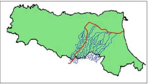
By overlapping the map of flood danger (L. Zamboni, 2015) with the Reno catchment boundaries (Fig.1) it is possible to recognize the responsibility of the Reno river in the occurrence of the most frequent flood events in the plain regions. Considering the typical characteristics of torrential rivers such as the Reno one (narrow river bad and steep slopes given by the mountain morphology of Apennines, high difference in elevation (almost 1900m) between the origin and the outlet just 60 km distant from each other), the result is that in case of heavy rain event over mountainous areas, the water flows forcefully and rapidly toward the plan fields in a quantity that may be so large to become a real danger
8
for activities and people living in those areas. The response time of the torrent system is so short that it may happen that hazardous discharges arrive on lowlands even before the precipitation that originates them in the mountains. In this scenario, it becomes extremely relevant to find methods that allow an extension of the lead-time of the river flow forecast, such as QPFs, which may enable a more timely implementation of warning systems to face the torrential events is safe conditions.
Fig.1 - Map of flood danger in Emili-Romagna. The Reno catchment and the Reno river are highlighted
3. RAINFALL-RUNOFF MODELS
Rainfall-Runoff (RR) model is a mathematical model which can simulate the relationship between the rainfall event over a catchment and the consequent river discharge. In simply words the model calculates the conversion of rainfall into runoff. The purpose is to get the river flow hydrograph given by an observed (or forecasted) rainfall event.
3.1 HISTORY OF RAIFALL-RUNOFF MODELS
Just to give a brief historic overview about the RR models development: the 1932 is widely recognized as the date in which the first rainfall runoff model was born. It was the so-called Unit Hydrograph: a technique providing a practical and relatively easy-to-apply tool to quantify the watershed response (in terms of runoff volume and timing) to a unit input (e.g. one cm) of rainfall. This is done through two strong hypotheses: rainfall event is uniformly distributed over the watershed and runoff response is linear and time-independent. Someone may argue that Rational Method was formulated firstly, in 1850, but considering the fact that it is not able to estimate the flow volume but just its peak value, we think that it based on too simple assumptions to be considered as a RR model. The Linear Reservoir Model represents a step forward. Indeed, it considers the energy balance conservation to establish the relationship between the storage and the runoff of a catchment. By the way, in order to solve the system of equations, the hypothesis of linearity is necessary: a too strong assumption for the purpose of representing the physical behaviour of the catchment.
Therefore, all these models are based on strong hypotheses and are reliable just for small and impervious catchments. In order to achieve a better physical interpretation of catchment response, the 1960s saw the development of Conceptual Models in which the basin is treated as an only entity with parameters that characterize its global behaviour. Moreover, the hydrologic cycle is represented by individual components that simulate the response of a particular subsystem. However, considering that those parameters were physically meaningless, there was the need to go ahead.
10
At the end of 1970s a new type of lumped model was introduced, based on the idea that rainfall-runoff process is mainly dominated by the dynamics of saturated areas. This is represented by a two-parameter distribution function curve representing the relation between the total volume of water stored in the soil and the extension of the saturated area (e.g. HYMOD model). Other processes represented in the model (drainage, percolation, groundwater flow, etc.) are based on empirical parameters that have to be estimated from data. The need to directly relate parameters with measurable quantities brought Beven and Kirkby in 1979 to elaborate a more physically meaningful distribution function model, the so called TOPMODEL. But the physically based hypothesis proved to be true only for very small hill-slope catchments (Franchini M., 1996). Therefore, Freeze and Harlan proposed a mathematical model based on distributed physical knowledge of surface and subsurface phenomena. In fact, by a numerical integration of the coupled sub-systems (surface flow, unsaturated and saturated subsurface flow) and by matching the solutions of each sub-system with the boundary conditions of another, a catchment scale prediction could be produced. But the cost to pay was the calibration of too many parameters. More recently, the wider availability of distributed information (radar rainfall, soil types, land cover, etc.) has facilitated the production of simplified physically meaningful distributed hydrological models (like TOPKAPI). These models, based on simplified assumptions (coupling conceptual and physical approaches) can be applied successfully to flood forecasting. In conclusion since the majority of models were developed after ‘90s, we can consider RR model application as a young science and therefore as a very active field of research.
3.2 HOW RAINFALL-RUNOFF MODELS WORK
The following sub-chapter is aimed to explain the basic concepts behind the functioning of rainfall-runoff model. By understanding these principles, we will realize how complex hydrological RR models as TOPKAPI work.
The mathematical model is nothing else than a system of equations in a number which is proportional to the number of variables that we want to simulate
(constitutive equations). Therefore, we need a minimum number of equations which is equal to the number of unknowns. Usually in this type of model variables are functions of time, since we want to simulate the behaviour of the catchment evolving in time. Hence, the final river flow output is not only a function of rainfall but also a function of time, therefore we consider it as a dynamic model. Otherwise in order to simulate the variables we are interested in, we may need to consider the state of the system. The latter one considers the hydrologic condition of the catchment at the time of the rain event (like drought and saturated conditions) and the variable which describe this is the storage. This relationship among variables: rainfall P(t) (input), river flow Q(t) (output) and storage W(t) (state of the system), can be conceptually associate with a bucket model (Fig. 2)
Fig.2 – conceptual association between the catchment and the bucket model
The amount of storage quantifies the state of the catchment: if W(t)=0 the catchment is dry, on the contrary if it reaches its maximum potential value the basin is completely saturated. Therefore, storage is a state variable and the introduction of it is necessary if we want to take into account the state of the catchment, thus two equations are needed for this specific case. Of course, the concept can be extended and the complexity of the model increases taking into account other states of the catchment, introducing additional state variables and equations.
Given that the purpose of this model is to describe the movement of water within the water cycle, equations are explicitly or implicitly based on physic laws. Examples of these equations are the conservation of energy, conservation of
12
mass and conservation of momentum. Moreover, by adding laws of chemistry, ecology, social science and so forth, it is possible to increase the complexity of the model taking into account other factors to better describe the dynamics of the catchment (changes in land-use/landcover, inclusion/removal of infrastructure, etc.)
Beside variables, constitutive equations may include parameters. They are numeric factors within the equations used in the model, which can assume different values in order to give flexibility to the model itself. To find the best value, for each parameter, that better describes the catchment it is necessary to calibrate the model. Nevertheless, in some models, parameters do not have a single fixed value, but they may change during the simulation depending on time or state of the system.
3.3 RAINFALL-RUNOFF MODELS CLASSIFICATION
The RR models used for flood forecasting may be classified in different categories. They can be distinguished basing on the way catchment processes are represented:
- Deterministic model: compute several equations representing the different watershed processes that produce a single model output for a given set of parameters;
- Stochastic model: provide the capability to simulate the random and probabilistic nature of inputs and responses that govern river flows. Deterministic model may be subdivided also according to the representation of the hydrological process within the catchment:
- Physically based model: the process of transformation of rainfall into runoff is time dependent and is function of the physical characteristics of the catchment.
- Conceptual model: describe the rainfall-runoff process in a more abstract and general way with respect to the physically based approach. In this way it has a simpler structure and more linearity in variables and parameters changes.
- Synthetic (or empirical or black-box) model: its purpose is not aimed to mathematically represent hydrologic and physical phenomena in the catchment. It considers the system as a closed box (black-box) on which there are specific hypothesis. Therefore, the model searches the mathematical operator that links rainfall to runoff in the best way possible.
An additional subdivision regards the spatial distribution of inputs and parameters:
- Lumped model: conceptualizes the catchment as a set of various storage tanks which represent different water storages within the catchment (superficial, unsaturated and groundwater zones). The model describes how the water moves through these tanks with a set of expressions; - Distributed model: the catchment is divided in cells. For each one of
them the basin properties are represented with specific parameters for that particular cell. In this way distributed model generally reproduces the hydrological processes within the catchment in a spatially-varied way.
Further classification account for the estimation of the rainfall for the lead time: - Updating model: involves the use of real-time data as input of the model.
In this way the model is more accurate and more reliable.
- Non-updating model: uses the rainfall input just on the basis of observed data.
It is important to state that the above classifications are not rigid and it is difficult to assign unequivocally a model just to a category.
14
4. TOPKAPI MODEL
TOPKAPI is an acronym which stands for TOPographic Kinematic APproximation and Integration. It is a fully distributed model in the sense that it considers the catchment with a grid cell discretisation for each of which the structure of the model is applied. The term physically based is used because of the capability of the model to represent on the catchment the hydrological processes described by the fluid mechanics and soil physics. The input parameters required are relatively few (15), only three or four of which typically require calibration (Liu & Todini, 2002). The chapter presents the main aspects of the model concerning its principles and physical concepts.
4.1 STRUCTURE AND METHODOLOGY
The model is based on the idea of combining the kinematic approach with the topography of the catchment. The Digital Elevation Model (DEM) subdivides the basin domain in squared cells, whose size generally increases with the overall dimension of the basin (pixel size is generally between 100 and 1000m). Therefore, the drainage network is evaluated according to the principle of minimal energy cost (Band, 1986) comparing the elevation of each cell with the ones of its neighbourhood cells. In particular, according to the TOPKAPI eight direction scheme, the links between the active cell and the eight surrounding is evaluated: the active cell is assumed to be connected downstream with a sole cell, while it can receive upstream contributions up to seven cells. In this way flow paths and slopes are evaluated. Moreover, for every grid cell of the DEM is assigned a value for each of the physical characteristics (parameters) represented in the model. Therefore, the spatial distribution of parameters, the precipitation input and the hydrological response are described in the horizontal direction by the grid scheme just obtained and in vertical by a column of soil for each grid square.
TOPKAPI proposes a single layer soil model in which the soil is considered with a limit thickness (usually 1 or 2 meters) and high hydraulic conductivity (because of the macro pores structure of the top layer soil). It contributes to the horizontal
flow (surface runoff) if its soil moisture content exceeds its saturation level (Todini E. , 1995), otherwise if its moisture content exceeds its field capacity, it loses water by percolation toward the deeper soil. The model does not consider the mechanism of infiltration at that depth and the consequently recharge to aquifers, the reason is that typically deep groundwater flows are long time events and their contribution to surface discharge of the catchment is observable only in a long-time scale (years). Therefore, since this study considers the discharge behaviour of the catchment on a shorter temporal window, it is reasonable to consider the water which exits from the soil cell (percolation) as lost from the model. The following conceptual scheme depicts the main structure of the model (Fig.3) regarding the interactions among three main reservoirs. The components of evapotranspiration, snowmelt and percolation will be discussed further. TOPKAPI is constructed around seven components: surface flow, groundwater flow, channel flow, evapotranspiration, snowmelt, percolation as well as lake/reservoir routing (this one is not considered in the present study). All the components may be considered for each grid cell of the DEM. The model is based on the hypothesis that sub-surface flow, overland flow and channel flow can be approximated using a Kinematic Wave Approach. The integration in space of the consequently non-linear Kinematic Wave equations, representing the three horizontal flow components (sub-surface, overland and channel), results in three “structurally-similar” non-linear reservoir differential equations (Liu Z. , 2002).
4.2 MODEL ASSUMPTIONS
The TOPKAPI model is based on 6 fundamental assumptions:
1. Precipitation is constant over the single grid cell, by means of area-distribution techniques (Thiessen polygons and Black Kriging) 2. All the precipitation falling on the soil infiltrates into it, unless the
soil in a particular zone (intended as cell) is already saturated: the saturation runoff mechanism, often called Dunne Mechanism (T.Dunne, 1978).
16
3. The slope of the water table coincides with the slope of the ground. This is the fundamental assumption of the Kinematic wave approximation in the Saint-Venant equation. Indeed, the model adopts the Kinematic wave propagation equation to describe the behaviour of horizontal flow in the unsaturated areas.
4. Local transmissivity, like horizontal subsurface flow in a cell, depends on the integral of the total water content of the soil in the vertical direction.
5. In the soil surface layer, the saturated hydraulic conductivity is constant with depth and, because of macro-porosity, is much larger than that of deeper layers.
6. During the transition phase, the variation of water content in time is constant in space.
4.3 MODEL EQUATIONS
The equations that for each cell define the interactions among the three main reservoir (soil, overland and channel reservoirs) are obtained by combining the physically-based and mass continuity equations under the approximation of the kinematic wave approach. The achieved differential equations are then analytically integrated in space to the finite dimension of the grid cell. For a fully detailed description of the theory which stands behind the resolution of these equations, it is suggested the analysis of the papers written by Liu and Todini (Liu & Todini, 2002). Just an overview aimed to understand the main relationship between equations is discussed below.
For each of the three reservoirs, the equation of mass continuity (of which a generic cell i is composed) can be written as a classical differential equation of continuity: 𝑑𝑉𝑖 𝑑𝑡 = 𝑄𝑖 𝐼𝑁− 𝑄 𝑖𝑂𝑈𝑇 (1) where:
- 𝑉𝑖 : total volume stored in the reservoir - 𝑑𝑉𝑖
- 𝑄𝑖𝐼𝑁 : total inflow contribution to the reservoir - 𝑄𝑖𝑂𝑈𝑇: total outflow contribution to the reservoir
The assumption of kinematic wave approximation leads to neglect the acceleration terms in the Saint-Venant energy equation and therefore it is possible to resolve the continuity and mass balance equations by assuming a non-linear relationship between 𝑄𝑖𝑂𝑈𝑇 and 𝑉𝑖 transforming Eq. (1) into an Ordinary
Differential Equation (ODE):
𝑑𝑉𝑖
𝑑𝑡 = 𝑄𝑖 𝐼𝑁− 𝑏
𝑖𝑉𝑖𝛼 (2)
where:
- 𝑄𝑖𝐼𝑁 : combination of the forcing variables which are depending on the reservoir type (soil, overland, channel). Represents the interconnecting flows between the element storage reservoir (cell) with upstream connected cells, including rainfall and evapotranspiration.
- 𝑏𝑖 : function of geometrical and physical characteristics of the reservoir - 𝛼 : function of geometrical and physical characteristics of the reservoir For each cell, at each time-step 𝑡 of the simulation, the 𝑄𝑖𝐼𝑁 inflow rate is computed, assuming that it is constant over the whole interval ∆𝑡, then the Eq. (2) is solved by numerical integration. The method used by TOPKAPI to solve the ODE equation is a hybrid approach between the Runge-Kutta-Fehlberg (RKF) method and the quasi-analytical solution (QAS). The RKF is used because of its adaptive time step algorithm that is widely recognised as one of the most numerically stable algorithms to solve ODEs equations in forward difference mode (Weatley, 1994). Moreover, its additional function, with respect to the original Runge-Kutta algorithm, allows to estimate the error at each computational step. To the other hand the QAS method is proposed by Liu and Todini (2002) because of its quicker computational time with respect to RKF. Therefore, the hybrid method is based on the QAS method as default procedure, and switches to the RKF algorithm when the mass continuity equations (Eq.(1)) are not satisfied. In this way it is possible to reduce the computation time of more than 50% compared with a RKF application used on its own. Table 1 shows for
18
each reservoir all the variables that are computed from the ODE. In order to better understand the connections among reservoir inflows and outflows, the Fig.3 illustrates the scheme of a typical modelled cell (note that for sake of clarity the figure neglects the evapotranspiration processes).
Drainage coefficient
In situations where a grid cell is described by a slope (𝑡𝑎𝑛𝛽1) in direction 𝑥 and a different slope (𝑡𝑎𝑛𝛽2) in direction 𝑦 (Fig.3), the local
conductivity coefficient 𝐶 (which defines the value of b factor in the Eq.(2)) is multiplied by a drainage coefficient 𝜎:
𝜎𝑆 = 1 +𝑡𝑎𝑛𝛽2
𝑡𝑎𝑛𝛽1 Soil Drainage Coefficient
𝜎𝑂 = 1 + (𝑡𝑎𝑛𝛽2
𝑡𝑎𝑛𝛽1) 1 2
Overland Drainage Coefficient
The coefficient is automatically computed by TOPKAPI on the basis of pixel elevation. The use of drainage coefficients increases the amount of water moving either in the sub-surface soil layer and on the surface; as a consequence, the amount of water that gets into the drainage network increases too.
Flow partition coefficient (FP)
The total outflow from the soil and from the overland (𝑄𝑆𝑂𝑈𝑇+ 𝑄𝑂𝑂𝑈𝑇) is partitioned between the downstream cell and the channel network according to the flow partition coefficient (𝐹𝑃). It represents the
percentage of soil and overland flow flowing toward the channel, namely in the direction that is perpendicular to that of the channel and parallel to that of the outflow pixel. In the study it has been decided to assign the value of 0.5 to the flow partition coefficient in order to split in half the outflow of either soil and overland reservoirs.
20 Fig .3 – Wa ter bal anc e a m ong t hr ee r es er v oi rs
4.4 EVAPOTRANSPIRATION COMPONENT
The most physically realistic model for estimating actual evapotranspiration is the Penman-Monteith equation, which has been widely used in many distributed models. However, due to the difficulty to get real-time data for Penman-Monteith estimations in operative flood forecasting applications, a simplified approach is generally necessary. Indeed, evapotranspiration plays a major role not in terms of its instantaneous impact, but in terms of its cumulative temporal effect on the soil moisture volume depletion; this reduces the need for an extremely accurate expression, provided that its integral effect is well preserved. Therefore, a simplified empirical equation such as the Thornthwaite method is used to get the reference potential evapotranspiration ET0, computed on a monthly basis: 𝐸𝑇0(𝑚) = 16 𝑎(𝑚) [10 𝑇(𝑚) 𝑏(𝑚)] 𝑐 (3) with: 𝑎𝑀 = 𝑛𝑀 30 𝑁𝑀 12 𝑏𝑀 = ∑ [ 𝑇𝑀 5] 1.514 12 𝑀=1 𝑐 = 0.49239 + 1792 ∙ 10−5𝑏 − 771 ∙ 10−7𝑏2+ 675 ∙ 10−9𝑏3 where:
- 𝐸𝑇0(𝑚) : reference potential evapotranspiration in the month 𝑚 - 𝑇(𝑚) : average air temperature in the month 𝑚
- 𝑁(𝑚) : maximum number of sunshine hours in the month 𝑚 - 𝑛(𝑚) : number of days in the month 𝑚
- 𝑚 = 1,2, … , 12 [months]
The developed relationship is linear in temperature and permits the desegregations of the monthly results on a daily or even on an hourly basis.
22
Once 𝐸𝑇0 has been computed on a monthly basis, the following empirical
equation is used to relate it to the compensation factor 𝑊𝑡𝑎, the average temperature (recorded) of the month 𝑇 and the maximum number of hours of sunshine 𝑁 of the month.
𝐸𝑇0(𝑚) = 𝛽(𝑚) 𝑁(𝑚) 𝑊𝑡𝑎𝑇(𝑚) (4)
where:
- 𝑇(𝑚) : monthly-average ait temperature in the month 𝑚 - 𝑊𝑡𝑎 : weighting factor for the radiation effects
- 𝑁(𝑚) : maximum number of sunshine hours in the month 𝑚 - 𝑚 = 1,2, … , 12 [months]
- 𝛽(𝑚) : regression coefficient for the month 𝑚
Once the values of coefficient 𝛽 is obtained for each month 𝑚, the values of 𝑇, 𝑊𝑡𝑎, 𝑁 and 𝛽 itself can be now used to estimate 𝐸𝑇0, instead of Thorntwaite formula. In particular 𝛽 is used to obtain the potential evapotranspiration values (ETP) by a simplified equation derived from the radiation method (Doorenbos J. P., 1984).
𝐸𝑇𝑃 = 𝐸𝑇0 ∙ 𝐾𝐶𝑐𝑟𝑜𝑝 (5) In particular since we are interested to obtain the 𝐸𝑇𝑃 value for each cell, for
each month of the year, for any crop at any time step ∆𝑡, Eq.(5) becomes 𝐸𝑇𝑃 = [𝛽 𝑁 𝑊𝑡𝑎𝑇∆𝑡] ∙ 𝐾𝐶𝑐𝑟𝑜𝑝 ∙ ∆𝑡 30 ∙ 24 ∙ 3600 (6) where: - ∆𝑡 : time interval [s] - 𝐾𝐶𝑐𝑟𝑜𝑝 : crop factor
- 𝑇∆𝑡 : average air temperature over the cell 𝑖 in ∆𝑡 [°C]
For different types of land use, monthly crop coefficients are given, reflecting the state of the plants in annual growth cycle (Doorenbos & Pruitt, 1992).
In fact, different evapotranspiration capacities of land uses are affected by the transpiration and evaporation from the water intercepted by the given vegetation. Finally, the potential evapotranspiration value is corrected as a function of the actual soil moisture content to obtain the actual evapotranspiration (EPA).
𝐸𝑇𝐴 = {
𝐸𝑇𝑃 𝑉
𝛽𝑉𝑠𝑎𝑡 𝑓𝑜𝑟 𝑉 ≤ 𝛽𝑉𝑠𝑎𝑡
𝐸𝑇𝑃 𝑒𝑙𝑠𝑒𝑤ℎ𝑒𝑟𝑒 (7) where:
- 𝑉 : actual volume of water stored into the soil [m3]
- 𝑉𝑠𝑎𝑡: local saturation volume [m3]
- 𝛽 : percentage of the saturation volume
The evapotranspiration losses are taken in account by the model by subtracting them both from the channel outflow rate, and from the soil or overland outflow depending on saturation conditions: if the cell is fully saturated evapotranspiration is taken off from the overland outflow rate, on the other hand evapotranspiration is extracted from the soil store alone. In particular:
𝐸𝑇𝐴 = {𝐸𝑇𝑃 𝑉
𝛽𝑉𝑠𝑎𝑡 𝑓𝑜𝑟 𝑠𝑜𝑖𝑙 𝑜𝑣𝑒𝑟𝑙𝑎𝑛𝑑 𝑟𝑎𝑡𝑖𝑜⁄ 𝐸𝑇𝑃 𝑓𝑜𝑟 𝑐ℎ𝑎𝑛𝑛𝑒𝑙 𝑟𝑎𝑡𝑖𝑜
4.5 SNOWMELT COMPONENT
For reasons of limited data availability, the snowmelt module within TOPKAPI is driven by a radiation estimate based upon the air temperature measurements; in practice, inputs to the snow module are precipitation, air temperature, and the same radiation approximation which was used in the evapotranspiration module. The principle is that as precipitation falls on the catchment, the snow accumulation and melting component identify the amount of water that actually reaches the soil surface.
At each model pixel snowmelt is computed by following five steps, on the basis of a snow pack energy and mass balance.
24 1. Net solar radiation estimation
The estimation of the radiation for each DEM grid (Eq.(8))is performed by re-converting the latent heat (which has already been computed previously as the reference evapotranspiration 𝐸𝑇0) to radiation (Eq.(9)).
𝑅𝑎𝑑 = 𝜆𝐸𝑇 + 𝐻 (8) where:
- 𝑅𝑎𝑑 : net solar radiation - 𝜆𝐸𝑇 : latent heat flux - 𝐻 : sensible heat
𝜆𝐸𝑇 = 𝐶𝑒𝑟 ∙ 𝐸𝑇0 (9) with:
𝐶𝑒𝑟 = [606.5 − 0.695(𝑇 − 𝑇0)] where:
- 𝐶𝑒𝑟 : conversion factor [Kcal/Kg]
- 𝑇0 : fusion temperature of ice [273 °K] - 𝑇 : air temperature [°K]
- 𝐸𝑇0: potential reference evapotranspiration
According to empirical tests applied within the TOPKAPI approximations, it is possible to compute the sensible heat as:
𝐻 = 𝜆𝐸𝑇 (10) Therefore:
𝑅𝑎𝑑 = 2 ∙ [606.5 − 0.695(𝑇 − 𝑇0)]𝐸𝑇0 (11)
In addition it is necessary to account for another factor which plays an extremely important role in snowmelt: Albedo. It is taken into account by which an efficiency factor (a function of Albedo).
Albedo (or reflection coefficient) is the diffuse reflectivity, or reflecting power, of a surface. It is the ratio of reflected radiation from the surface to incident radiation upon it. It is dimensionless and it is measured on a scale from zero (for no reflection of a perfectly black surface) to 1 (for perfect reflection of a white surface). In TOPKAPI model an average Albedo value is used to compute the efficiency factor for clear sky and overcast conditions according to the following empirical equations:
𝜂𝑐𝑙𝑒𝑎𝑟 = 1 − 𝐴𝑙𝑏𝑒𝑑𝑜
𝜂𝑜𝑣𝑒𝑟𝑐𝑎𝑠𝑡= (1 − 𝐴𝑙𝑏𝑒𝑑𝑜) ∙ 1.33
Default value is Albedo=0.4, which brings =0.6 for clear sky (when not raining or snowing) and =0.8 for overcast conditions (when raining or snowing).
2. Estimation of solid and liquid precipitation amount
On the basis of air temperature, TOPKAPI estimates the percentage of liquid precipitation using the following function:
𝑅𝑎𝑖𝑛%(𝑇) = 1
1+𝑒𝑇𝐴𝐼𝑅−𝑇𝑆0.6
(13)
where:
- 𝑇𝑆 : threshold temperature, fixed to 0°C
- 𝑇𝐴𝐼𝑅 : air temperature
3. Estimation of the water mass and energy budgets based on the hypothesis of zero snowmelt
A tentative value for mass and energy of the snowpack is computed at time 𝑡 + ∆𝑡 (with the hypotesis of zero snowmelt):
Tentative mass balance : 𝑍𝑡+∆𝑡∗ = 𝑍𝑡+ 𝑃 (14) Tentative energy balance:
26
Rain: 𝐸𝑡+∆𝑡∗ = 𝐸𝑡+ 𝑅𝑎𝑑 + [𝐶𝑠𝑖𝑇0 + 𝐶𝑙𝑓+ 𝐶𝑠𝑎(𝑇 − 𝑇0)]𝑃 (16)
where:
- 𝑍𝑡 : water equivalent mass at time 𝑡 [mm] - 𝑃 : precipitation [mm]
- 𝐸𝑡 : energy at time 𝑡 [mm] - 𝑅𝑎𝑑 : net solar radiation
- 𝐶𝑠𝑖 : specific heat of ice [= 0.5 𝐾𝑐𝑎𝑙 °𝐾 ∙ 𝐾𝑔⁄ ]
- 𝐶𝑙𝑓 : latent heat of fusion of water [= 79.6 𝐾𝑐𝑎𝑙 𝐾𝑔⁄ ]
- 𝐶𝑠𝑎 : specific heat of water [= 1 𝐾𝑐𝑎𝑙 °𝐾 ∙ 𝐾𝑔⁄ ] - 𝑇 : air temperature
- 𝑇0 : temperature of snowmelt [=0 °C]
4. Comparison between the tentative snow energy and the total available one
The tentative energy balance for the snow, computed at 273 °K considering the total available mass, is compared with the total available energy in order to decide if the snowpack is going to melt or not.
𝐸𝑡+∆𝑡∗ { ≤ 𝐶𝑠𝑖𝑍𝑡+∆𝑡∗ 𝑇0 𝑡ℎ𝑒 𝑡𝑜𝑡𝑎𝑙 𝑒𝑛𝑒𝑟𝑔𝑦 𝑖𝑠 𝑛𝑜𝑡 𝑒𝑛𝑜𝑢𝑔ℎ 𝑓𝑜𝑟 𝑚𝑒𝑙𝑡𝑖𝑛𝑔 𝑡ℎ𝑒 𝑠𝑛𝑜𝑤𝑝𝑎𝑐𝑘 > 𝐶𝑠𝑖𝑍𝑡+∆𝑡∗ 𝑇0 𝑡ℎ𝑒 𝑡𝑜𝑡𝑎𝑙 𝑒𝑛𝑒𝑟𝑔𝑦 𝑖𝑠 𝑒𝑛𝑜𝑢𝑔ℎ 𝑓𝑜𝑟 𝑚𝑒𝑙𝑡𝑖𝑛𝑔 𝑡ℎ𝑒 𝑠𝑛𝑜𝑤𝑝𝑎𝑐𝑘
5. Computation of the snowmelt produced by the excess energy
When the total energy is not enough to melt the snowpack, the water mass and energy budget are updated:
𝑅𝑠𝑚 = 0 𝑍𝑡+∆𝑡 = 𝑍𝑡+∆𝑡∗ 𝐸𝑡+∆𝑡 = 𝐸𝑡+∆𝑡∗
To the other hand, if the energy is sufficient to melt the snowpack, the amount of snow that is transformed into water (𝑅𝑠𝑚) is computed:
𝑅𝑠𝑚 =𝐸𝑡+∆𝑡∗ −𝐶𝑠𝑖𝑍𝑡+∆𝑡∗ 𝑇0
𝐶𝑙𝑓 (17)
𝑍𝑡+∆𝑡 = 𝑍𝑡+∆𝑡∗ − 𝑅𝑠𝑚
𝐸𝑡+∆𝑡= 𝐸𝑡+∆𝑡∗ − (𝐶𝑠𝑖𝑇0+ 𝐶𝑙𝑓)𝑅𝑠𝑚
4.6 PERCOLATION COMPONENT
For the deep aquifer flow the response time, caused by the vertical transport of water through the thick soil above this aquifer, is so large that horizontal flow in the aquifer can be assumed to be almost constant with no significant response on one specific storm event in a catchment (Todini E. , 1995). Nevertheless, the TOPKAPI model accounts for water percolation towards the deeper subsoil layers even though it does not contribute to the discharge, but simply as a lost outflow from the soil cell.
The percolation rate from the upper soil layer is assumed to increase as a function of the soil water content according to an experimentally determined power law (Clapp & Hornberger, 1978) but not to exceed the saturated soil hydraulic conductivity in the underlying deeper layer.
𝑃𝑟 = 𝑘𝑠𝑣( 𝑣 𝑣𝑠𝑎𝑡) 𝛼𝑃 (18) 𝑣𝑠𝑎𝑡(𝜗𝑠− 𝜗𝑟)𝐿𝑋 (19) where: - 𝑃𝑟 : percolation [mm]
- 𝑘𝑠𝑣 : vertical soil saturated conductivity [m3/s] - 𝑣 : volume [m3]
- 𝑣𝑠𝑎𝑡 : local saturation volume [m3]
- 𝛼𝑃 : vertical non-linear reservoir exponent
𝛼𝑃 depending on the type of soil: may varies between 11, typical value for a
28
5. CASE STUDY: CATCHMENT DESCRIPTION
The chapter aims to describe the catchment physical characteristics looking for each component of the basin. A general overview of the geography, lithology and morphology, coupled with the meteorological considerations, is aimed to understand the hydrological behaviour of the catchment in order to better represent it with a mathematical model.
5.1 RENO CATCHMENT
Reno river is the tenth Italian river in terms of length (212 km) and basin extension (5040 km2). These characteristics make him the major river, considering also the average discharge at the outlet, among those flowing into the Adriatic Sea on the south of the Po river. The majority of the basin is included in the Emilia-Romagna region (4467 km2 hence the 88,4% of the whole Reno catchment). In Emilia-Romagna are incorporated the towns of Bologna (68,5%), Ravenna (17,7%), Modena (1,3%) and Ferrara (0.9%). Despite its huge dispersion in Emilia-Romagna, the Reno river originates in the Tuscany region: conventionally at the junction of two rivers (Reno di Prunetta and Reno di Campolungo) at 745 m a.s.l. The Tuscan territory within the catchment is 573 km2 (11.6% of the whole basin) and are interested the towns of Florence (7.7%), Pistoia (3.1%) and Prato (0.8%) (Distretto Idrografico Appennino Settentrionale, 2010).
It is inhabited by nearly 2 million of peoples and includes areas with high concentration of industries (e.g. the metropolitan area of Bologna) and agricultural fields (e.g. area surrounding Lugo-Massa Lombarda for the production of fruit) (Fig.4 - source (Distretto Idrografico Appennino Settentrionale, 2010)).
The mountainous basin is extended for 2540 km2, in this territory rainfall water flows on the mountain slopes converging into streams for all the drainage basin until the main river is shaped. Considering just this mountainous part of the catchment it measures 1061 km2 with a maximum elevation of 1945 m a.s.l. and a minimum one of 60.35 m a.s.l. (at the gauge station at Casalecchio di Reno).
The mountain part of Reno catchment is composed by 8 principal rivers; 12 secondary rivers and 600 minor rivers.
Fig.4 – hydrographic network and main urban settlements in the Reno catchment
As far as concerned the plain territories, the actual drainage basin of the Reno river is the result of different anthropogenic transformations, created for the purposes of hydraulic defence and reclaim of swamp areas in order to urbanize this plain part of the region. This historical evolution has determined among centuries a radical change in the territories between Bologna, Ferrara and Ravenna: the water streams which come from the Apennines and pass Via Emilia, flow within artificial embankment toward the Adriatic Sea for 124 km.
5.2 HYDROGRAPHY OF THE CATHCMENT
The catchment of the Apennines in the Bologna’s area is mostly made of rivers originated in the Apennines’ crest region, flowing until the end of the mountainous relief. They maintain an opposite direction with respect to the Apennines’ one and being mostly parallel among themselves (Fig.5 - source (Wikipedia, 2019)).
30
Fig. 5 – Hydrography of the Reno catchment
The rivers in this area are characterized by a torrential stream with peak flows in the period between late Autumn, Winter and early Spring (in particular December, February and March). This discharge value is much higher, even double, compared with the summer months. The reason is the type of alimentation which is almost entirely given by rainfall; just a minor part is composed by the superficial water equivalent made by the snow melt. Nevertheless, the dominant impermeable nature of soils is the reason of the balance between outflows and inflows, but there are some exceptions. For instance, in September is measured the minimum runoff coefficient value (0.16) because of the water losses given by dry soils presence, which are typical of the autumnal dry weather and the hot one in summer. Therefore, the discharge peak value is not measured in correspondence of the maximum outflow (in November) but later, in March, because of the water contribution from the snow melt.
5.3 RIVER CLASSIFICATION
All Reno’s tributaries are characterized by a recognisable catchment individuality. Is possible to identify a main catchment, 5 other sub-basins and other smaller rivers, all part of the Reno’s catchment (Fig.6 - source (Barbieri, s.d.)). Rivers are classified on the basis of the sub-basin extension, indeed to this
size is related the average maximum discharge value. The classification can be summarized as follow:
- Principal rivers: the ones with a catchment grater or equal to 40 km2 - Secondary rivers: the ones with a catchment in between 40 and 13 km2. - Minor rivers: all those streams which are not included in the previous classification, showed in the Technical Regional Cartography with a scale of 1:5000.
Fig.6 – sub-basin identification within the Reno catchment
5.4 GEOMORPHOLOGICAL ASSET
According to lithological, stratigraphic, structural and morphological characteristics, it is possible to subdivide the Reno catchment in 5 sectors:
- Apennine Ridge: in correspondence of the Tyrrhenian-Adriatic watershed is made by turbidite sedimentary deposits, arenaceous-pelitic rocks characterized by a quartzous-feldspathic composition, with schistic-clayey-marly base and interposition of sandstones and limestones. The landscape is characterized by deep torrential furrows and
32
rocky outcrops coming out from the cliffs. Here are localized the upper part of the principal drainage basins.
- Apennine of Emilia: the is the mid-west portion of the Reno catchment. Is the area mostly interested by deformations which cause high slope instability (because of the low mechanical properties of the outcrop rocks). Is characterized by sedimentary rocks composed by a chaotic structure of clay and limestones with inclusions of sandstone. Hence, landslides are caused by mud flows which may interrupt river paths causing their deviation and the erosion of embankments. There are also others rock formations like the so-called “Ligurian Flish” (a turbidite sequence of marly-limestone rocks and arenaceous-pelitic formations) and “Epiligure Sequence” (marlstones of different colours and
quartzous-feldspathic sandstones). The poor mechanic characteristics of these rocks interest both the superficial layer and the substrate giving to the slopes a characteristic corrugated shape with concavities and convexities.
- Lower Apennine: defines the northern mountainous part of the catchment arriving until the lowland. Is characterized by modest heights and high geomorphological dynamicity (due to the low resistance of outcropping rocks). In correspondence of the main rivers there are large terraced surfaces typical of the landscapes like Badlands (Calanchi) and karst regions.
- Apennine of Romagna: the east-side part of the catchment, defined by arenaceous-pelitic deposits originating in the Alpes. In general, this sector is less tectonically deformed with respect the previous ones and landslides are made mostly by rocks (rarely by mud) in correspondence of the principal tectonic structures.
- Lowland: from the Apennines boundary until the Adriatic Sea, it is part of the Pianura Padana. The actual conformation of the latter is given by climate changes caused by the last ice age of roughly 10.000 years ago and the consequent sea level fall shaping the current coast line. At the
basis of its origins there was two different lithological processes: the alluvial plain and the river delta plain.
Therefore, an overall panoramic of the morphology depicts the upstream part of the catchment (a third of the whole basin) made of resistant limestones and sandstones. This relatively easy erodible part represents the sub-Ligurian folded rock units (nappes), that have been exposed by erosion and removal of the Ligurian cover-rock. Surface mechanisms in this area consist of debris flow and mass wasting of Pleistocene glacial deposits. On the contrary the downstream two-thirds of the catchment consist on relatively thin Pliocene-aged sandstones acting like a caprock for the wide spread marls, mudstones, siltstones and silty sandstones typical of the Ligurian and Epiligurian units. Because of the impermeable and erodible characteristics of these rocks, in addition to the heavy rainfall periods on which this area is subjected, this part of the catchment is marked by Badlands (Calanchi), originated from runoff processes, causing soil erosion and landslides. In conclusion the morphology of this areas differs among steep slopes covered by woods and low hills with grasslands.
5.5 HYDROLOGIC ASSET
Given the impermeable characteristics of the lithological structure of the catchment, all the rivers in the mountainous area are defined by a torrential stream. As a consequence, the trend of discharges in the basin reflects the one of precipitations, with some exceptions in winter and spring due to snow melt. The average annual discharge for the Reno varies between 15 to 26 L/sec (Reno, 2002). At the gate station of Casalecchio di Reno the average annual discharge is 26 m3/s, instead at the outlet of Casalborsetti is 95 m3/s. The average measured value for flooding events is just barely above 1000 m3/s, usually registered in March. Minimum values are 4 m3/s at Casalecchio and 0.6 m3/s at Casalborsetti, even if less than a century ago the minimum discharge was never less than 5 or 6 m3/s. The latter datum depicts that the river, especially in mountainous areas, is strongly exploited among years for human purposes (domestic and irrigation). The hydrography of the catchment was altered by the construction, on the
34
tributaries of the main stream of the Reno river, of five large hydroelectric dams (Suviana, Brasimone, Pavana, Santa Maria and Molino del Pallone) with a total capacity of 52x106 m3. Almost all the reservoirs are linked together by underground channels.
5.6 LAND USE
Land cover of the catchment is dominated by woods. This is the result of the reforestation operations started in the 1950s and proceeding nowadays as a consequence of mountain areas abandonment. The result is that the wood percentage has increased from 24% to 60% in between 500 m to 900 m a.s.l. and from 70% to 98% above 900 m a.s.l. The upper part of the catchment is mainly covered by chestnuts, oaks and beeches, while hillsides are characterized by coppices, pastures (especially at higher altitudes), shrubs and crops. Regarding the agricultural landscape the post-war scenario defines the abandonment on mountainous areas. In fact, the technological agricultural improvements lead to prefer flat fields (Pianura Padana) with respect to mountainous cultivated areas, which face a reduction from almost 40% to 5% (D.Pavelli, 2013). The valley is covered by crops, vineyards, orchards and urban areas.
5.7 CLIMATIC CLASSIFICATION
Falling within the Apennine climatic zone, the Reno catchment is characterized by two periods of high precipitations (autumn and spring) and one period of low precipitations (summer) when, between June and August, a long dry season persists. The average annual precipitation measured on a date set of 81 years (D.Pavelli, 2013) from 1926 to 2006, is 1307 mm/year. Regarding the seasonal values, the mean precipitation is 355 mm in winter (December, January and February), 322.2 mm in spring (March, April and May), 194.0 mm in summer (June, July, and August) and 434.4 mm in autumn (September, October and November). From November to March, in the higher catchment areas, some snowfalls may occur.
6. CASE STUDY: MODEL CALIBRATION
The study defines the reliability of the model working with forecasting data in different scenarios: firstly, under some assumptions of predicted rainfall based on the observed one, then using forecasting data of precipitation in a real-time configuration. In order to do that, it is necessary to estimate the reliability of the spatial distribution of the rainfall with an analysis of spatial variability. Most importantly, the model needs to be calibrated and validated on a chosen period. As the Reno river has a torrential character at Casalecchio cross section, the simulations described here below consider only the upper part of the basin, which for sake of simplicity, from now on, will be called “Upper Reno catchment”.
6.1 PARAMETER REQUIREMENTS
The methodology to derive parameters for the TOPKAPI model from the Reno catchment information is based essentially on two main procedures:
- Determination of the catchment geometrical characteristics: the grid cell size, the cells composing the river network and how the cells are connected.
- Assignment of the parameter values that better represent the physical behaviour of the catchment.
Determination of geometrical information
As already stated in the previous chapter, the model requires the definition of a grid that divides the catchment space into squared cells that must be connected in order to model the surface and subsurface flows within the catchment. Therefore, the grid lateral dimension (X value in the model equations) is imposed with a resolution of 500m and the drainage network is defined by choosing the 8-direction scheme. At this point, using the DEM (Digital Elevation Model) file of the catchment it is possible to determine the outflow direction of each cell, and thus the direction of the steepest outflow path from an active cell to the neighbouring downstream cells. In particular, the method identifies the steepest
36
downslope flow path among each cell of a raster DEM and its eight neighbors, and defines this path as the only flow path leaving the raster cell. The final step to define the drainage network is selecting a threshold catchment area at the bottom of which a source channel originates; all cells with a catchment area greater than this threshold are classified as part of the drainage network. The threshold value chosen for the area is fixed at 0.25 km2. In reality, the extension of the drainage network changes within the season and depending on the flow intensities, but this value is considered to be an acceptable compromise. In fact, the value of 0.25 km2 is in accordance with Todini’s recommendation that the ratio between the number of channel cells and the total cells number should be a value ranging between 5% and 15% of the total catchment area (Todini, 1996). The drainage network is finally defined.
Physical model parameters
One of the advantages of the TOPKAPI model is its physical basis that allows the link between model parameters and catchment characteristics. All the parameters values, or range of values, used in this study are reported in the Table 2 as well as the references from where the values are taken.
The constant parameters (𝑋,Athreshold) are assigned, as already noted in the
previous section, as well as the 0.5 value fixed for the flow partition coefficient (𝐹𝑃) to split the overall cell outflow (overland + soil) into the channel contribution and the next downstrem soil contribution.
The slopes of the ground tan (𝛽) (𝛽1and 𝛽2 for the drainage coefficient) are
directly computed from the cell elevation of the DEM, as well as the values for the angle riverbed tan (𝛾) and the slopes used to transfer the flow in the channel drainage network tan (𝛽𝐶).
For the soil cell-specific parameters the soil map is mainly used to derive the values for the residual and saturated soil moisture content (𝜃𝑟, 𝜃𝑠), the soil depth
of the cell (𝐿), the horizontal and vertical permeability (𝐾𝑠, 𝐾𝑠𝑣) and the vertical non-linear reservoir exponent for percolation (𝛼𝑃). The pore-size distribution parameter for the horizontal flow in the soil cell is uniformly set to the value 2.5
(Liu & Todini, 2002). The ordering method of Strahler (1957) is used to infer the values of channel roughness Manning’s coefficients (𝑛𝐶). In Liu and Todini
(2002), channel orders of 1,2,3 and 4 are assigned with the respectively values 0.045, 0.04, 0.035 and 0.035 for the same Reno catchment. The overland roughness Manning’s coefficient (𝑛𝑜) is derived from the land use map as well as the value for the crop factor 𝐾𝐶.
6.2 DATA REQUIREMENTS
In order to define the morphological, physical and hydraulic characteristics of the basin, Tab.3 defines the maps used in the study and their references. Data concerning rain, temperature and discharge are given by regional agency ARPAE of Bologna and cover entirely the period from the beginning of 2005 to the end of 2013. A summary of gauges information is following given in Tab.4.
Precipitation Temperature Discharge
So
u
rce ARPAE Emilia-Romagna ARPAE Emilia-Romagna ARPAE Emilia-Romagna
Per io d 01/01/2005 – 31/07/2013 01/01/2005 – 31/07/2013 01/01/2005 – 29/01/2014 T im e
Step 1 hour 1 hour 1 hour
Statio n s n u m b er 109 56 18 Statio n s sp ac ial d is tr ib u tio n
38
Tab.2 – Value of TOPKAPI model parameters
Parameters Values Origin and References C o n stan t v alu es 𝑋
Lateral dimension of the cell
grid [m] 500
Athreshold Threshold catchment area
[km2] 0.25
𝐹𝑃 Flow Partition Coefficient 0.5 [0.0 – 1.0]
So
il
𝜃𝑟 Residual soil moisture content 0.004 – 0.1005 Soil Map
𝜃𝑠 Saturated soil moisture
content 0.3791 – 0.4973 Soil Map
𝐿 Soil depth [m] 0.3 – 2.72 Soil Map
𝛼𝑆 Horizontal non-linear
reservoir exponent 2.5 Liu and Todini (2002)
𝐾𝑆 Horizontal Permeability at
Saturation [m/s] 9.9E-007 – 1.32E-003 Soil Map
Overland 𝑛𝑜 Manning’s overland
roughness coeff. [m-1/3s-1] 0.03 – 0.28 Landuse Map
Channel 𝑛𝐶 Manning’s channel roughness
coeff. [m-1/3s-1] 0.02 – 0.075 Strahler’s order method
ET 𝐾𝐶 Crop Factor 0.2 – 1.25 Landuse Map
Sn
o
wm
elt 𝑇𝑆 threshold Temperature for snowfall / rainfall 0°C
Albedo Albedo or reflection
coefficient 0.4 [0.0 – 1.0]
Per
co
latio
n 𝐾𝑆𝑉 Vertical Pemeability at
Saturation [m/s] 9.9E-10 – 1E-07 Soil Map
𝛼𝑃 Vertical non-linear reservoir
T ab .4 – i npu t m aps f or t he T O P K A PI m odel