Comparison between different configurations of piezoelectric energy harvester from galloping instability

(1)

POLITECNICO DI MILANO

School of Industrial and Information Engineering

Master of Science in Mechanical Engineering

Comparison between different configurations of piezoelectric energy

harvesting from galloping instability

Supervisor: Prof. Gisella TOMASINI Co-Supervisor: Ing. Stefano GIAPPINO

Master’s Thesis of:

Giancarlo MARIANI Id. Number 863526

(2)

(3)

CONTENTS i

FIGURES

Figure 1.1 Example of micro-turbine. ...7

Figure 1.2 A prototype of micro-turbine proposed by Pray. ...7

Figure 1.3 Representation of the vortex shedding phenomenon...8

Figure 1.4 (a) the scheme of the prototype provides by Pobering [5] and (b) the prototype of Akaydin [6] ...10

Figure 1.5 Wind tunnel experiment of the flutter energy harvesting prototype provide by Chawdhury and Morgental [11] ...10

Figure 1.6 Schematic of wake galloping phenomenon [12] ...11

Figure 1.7 Scheme of galloping piezoelectric energy harvesting ...12

Figure 1.8GPEH prototypes. (a) transversal model [15], (b) 2DOF system [29] and (c) longitudinal model [14] ...14

Figure 1.9 GPEH configurations scheme. (a) transversal one beam, (b) transversal two beams and (c) longitudinal ...16

Figure 2.1 GPEH layout for a longitudinal configuration ...17

Figure 2.2GPEH layout for a transversal configuration with two cantilever beams ...17

Figure 2.3 Convention for the positive direction of stress, strain and bending moment for a beam with two PZT attached to a metal beam ...19

Figure 2.4 Representation of aerodynamic forces per unit length acting on a square-section bluff body ...20

Figure 2.5 Transversal Model ...25

Figure 2.6 Longitudinal Model ...25

Figure 2.7 Angle Attack ...39

Figure 2.8 Angle α transversal Model ...40

Figure 2.9 Example of decay ...43

Figure 2.10 Exact Vs Approximate Formulation ...44

Figure 3.1 Reference case CAD...51

Figure 3.2 Modal shape reference case ...52

Figure 3.3 Modal shape variation second region ...55

Figure 3.4 Effect of variation length second region...56

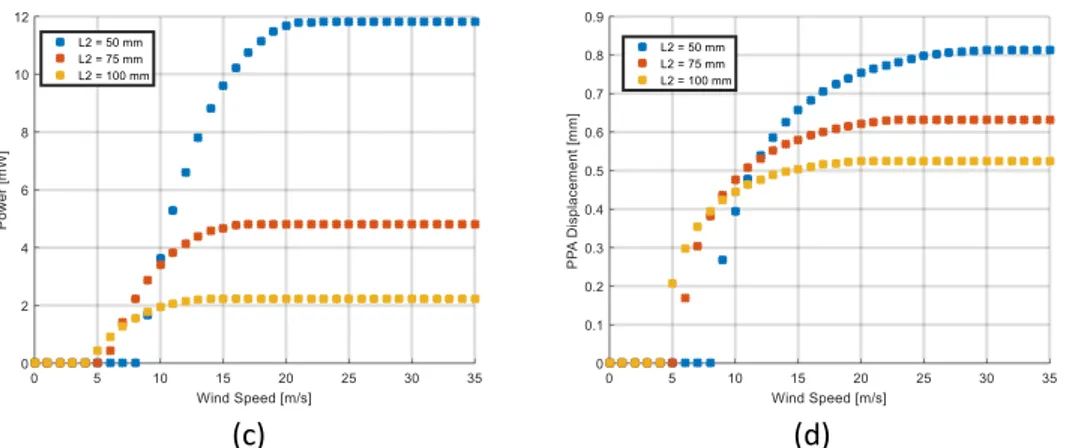
Figure 3.5 Time response variation second region. (a) Voltage Vs wind, (b) tip displacement Vs wind, (c) power Vs wind and (d) PPA displacement Vs wind ...57

Figure 3.6 Modal shape width beam variation ...58

Figure 3.7 Effect of variation width beam ...59

Figure 3.8 Time response variation width beam. (a) Voltage Vs wind, (b) tip displacement Vs wind, (c) power Vs wind and (d) PPA displacement Vs wind ...60

(7)

FIGURES

v Figure 3.9 Modal shape thickness beam variation ...61 Figure 3.10 Effect of thickness beam variation ...61 Figure 3.11 Time response thickness beam variation. (a) Voltage Vs wind, (b) tip displacement Vs wind, (c) power Vs wind and (d) PPA displacement Vs wind ...62 Figure 3.12 Modal shape material beam variation ...63 Figure 3.13 Time response material beam variation. (a) Voltage Vs wind, (b) tip

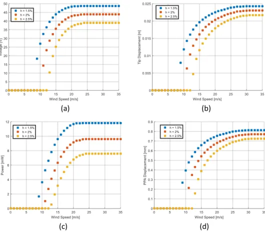
displacement Vs wind, (c) power Vs wind and (d) PPA displacement Vs wind ...64 Figure 3.14 Modal shape damping ratio variation ...66 Figure 3.15 Effect of damping ratio variation ...66 Figure 3.16 Time response material beam variation. (a) Voltage Vs wind, (b) tip

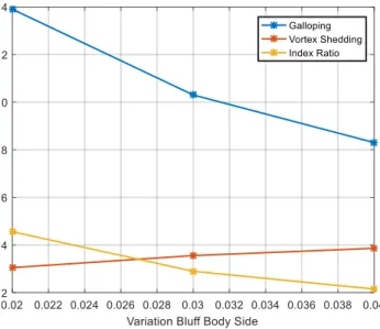
displacement Vs wind, (c) power Vs wind and (d) PPA displacement Vs wind ...67 Figure 3.17 Modal shape bluff body density variation ...68 Figure 3.18 Effect of bluff body density variation ...69 Figure 3.19 Time response bluff body density variation. (a) Voltage Vs wind, (b) tip displacement Vs wind, (c) power Vs wind and (d) PPA displacement Vs wind ...70 Figure 3.20 Modal shape bluff body length variation ...71 Figure 3.21 Effect of bluff body length variation ...71 Figure 3.22 Time response bluff body length variation. (a) Voltage Vs wind, (b) tip displacement Vs wind, (c) power Vs wind and (d) PPA displacement Vs wind ...72 Figure 3.23 Modal shape bluff body side variation ...73 Figure 3.24 Effect of bluff body side variation ...74 Figure 3.25 Time response bluff body side variation. (a) Voltage Vs wind, (b) tip

displacement Vs wind, (c) power Vs wind and (d) PPA displacement Vs wind ...75 Figure 3.26 Modal shape piezo patch variation ...76 Figure 3.27 Time response piezo patch variation. (a) Voltage Vs wind, (b) tip

displacement Vs wind, (c) power Vs wind and (d) PPA displacement Vs wind ...77 Figure 3.28 Modal shape number of beam variation ...78 Figure 3.29 Time response number of beam variation. (a) Voltage Vs wind, (b) tip displacement Vs wind, (c) power Vs wind and (d) PPA displacement Vs wind ...79 Figure 3.30 Modal shape resistance variation...80 Figure 3.31 Effect resistance variation ...80 Figure 3.32 Time response number of beam variation. (a) Voltage Vs wind, (b) tip displacement Vs wind, (c) power Vs wind and (d) PPA displacement Vs wind ...81 Figure 3.33 Time response number of beam variation. (a) tip displacement Vs

resistance, (b) power Vs resistance ...82 Figure 3.34 Modal shape different prototype ...83 Figure 3.35 Dimension of piezo patch PPA1011 ...85 Figure 3.36 Different longitudinal prototypes. (a) A40, (b) A30, (c) A20, (d) B20, (e) B30 and (f) B40...87 Figure 3.37 Different transversal prototypes. (a) C5 and (b) D9 ...88 Figure 4.1 (a) experimental setup scheme of a shaker and (b) shaker setup for

(8)

FIGURES

vi Figure 4.2 Experimental devices. (a) c-DAQ module and (b) electromechanical shaker ...92 Figure 4.3 (a) wind tunnel with prototype, (b) instrumentation used in wind tunnel ...94 Figure 4.4 Scheme of measurement acquisition points for longitudinal prototype ...96 Figure 4.5 Prototype scheme and shaker force ...97 Figure 4.6 Comparison between laser-accelerometer sensors for prototype A30 ...99 Figure 4.7 Motion-imposed tests: comparison between experimental and numerical results in term of FRF prototype A20 with R = 100 kΩ. (a) A Tip/A Constraint, (b) V PPA/A Constraint and (c) V PPA/L Tip ...101 Figure 4.8 Motion-imposed tests: comparison between experimental and numerical results in term of FRF prototype A20 with R = 10 kΩ. (a) A Tip/A Constraint, (b) V PPA/A Constraint and (c) V PPA/L Tip ...101 Figure 4.9 Motion-imposed tests: comparison between experimental and numerical results in term of FRF prototype A20 with R = 1 MΩ. (a) A Tip/A Constraint, (b) V PPA/A Constraint and (c) V PPA/L Tip ...102 Figure 4.10 Motion-imposed tests: comparison between experimental and numerical results in term of FRF prototype C5 with R = 100 kΩ. (a) A Tip/A Constraint, (b) V PPA/A Constraint and (c) V PPA/L Tip ...102 Figure 4.11 Motion-imposed tests: comparison between experimental and numerical results in term of FRF prototype D9 with R = 100 kΩ. (a) A Tip/A Constraint, (b) V PPA/A Constraint and (c) V PPA/L Tip ...103 Figure 4.12 Example of concentrated mass for (a) prototype A20 and (b) prototype A40 ...106 Figure 4.13 Analytical modal shape prototype A30 ...107 Figure 4.14 Piezo patch deformation for models B ...108 Figure 4.15 Modal shape comparison between analytical and experimental results for (a) A20, ...110 Figure 4.16 Example of decay on prototype A30 ...111 Figure 4.17 Interpolation for damping ratio (a) A20, (b) B30, (c) A40, (d) B40, (e) C5 and (f) D9 ...112 Figure 4.18 Numerical simulation to show the effect of the resistance load on the power ...113 Figure 4.19 Power response prototype A20 ...114 Figure 4.20 Wind tunnel tests: comparison between analytical and experimental results for prototype A40 (a) tip displacement vs wind, (b) PPA displacement vs wind and (c) power vs wind ...116 Figure 4.21 Wind tunnel tests: comparison between analytical and experimental results for prototype A30 (a) tip displacement vs wind, (b) PPA displacement vs wind and (c) power vs wind ...117 Figure 4.22 Wind tunnel tests: comparison between analytical and experimental results for prototype A20 (a) tip displacement vs wind, (b) PPA displacement vs wind and (c) power vs wind ...117

(9)

FIGURES

vii Figure 4.23 Wind tunnel tests: comparison between analytical and experimental results for prototype B40 (a) tip displacement vs wind, (b) PPA displacement vs wind and (c) power vs wind ...118 Figure 4.24 Wind tunnel tests: comparison between analytical and experimental results for prototype B30 (a) tip displacement vs wind, (b) PPA displacement vs wind and (c) power vs wind ...119 Figure 4.25 Wind tunnel tests: comparison between analytical and experimental results for prototype B20 (a) tip displacement vs wind, (b) PPA displacement vs wind and (c) power vs wind ...119 Figure 4.26 Different transient velocities for prototype B30 ...120 Figure 4.27 Wind tunnel tests: comparison between analytical and experimental results for prototype C5 (a) tip displacement vs wind, (b) PPA displacement vs wind and (c) power vs wind ...122 Figure 4.28 Wind tunnel tests: comparison between analytical and experimental results for prototype C5 (a) tip displacement vs wind, (b) PPA displacement vs wind and (c) power vs wind ...123 Figure 4.29 Wind tunnel tests: comparison between analytical and experimental results for prototype D9 (a) tip displacement vs wind, (b) PPA displacement vs wind and (c) power vs wind ...123 Figure 4.30 Moment study on prototype D9 ...125 Figure 4.31 Comparison between prototypes A40, D9 and B40 in terms of power recovered in function of wind speed ...127 Figure 4.32 Focused on PZT patch deformation from analytical modal shape for

prototypes C5 and D5 ...127 Figure 5.0.1 A non-perfect interaction between galloping and vortex shedding for prototype B40 in term of power in function of the wind speed...130

(10)

TABLES

viii

TABLES

Table 1.1 Summary of different small-scale windmills ...8

Table 1.2 Effect of the shape section on Strouhal number ...9

Table 1.3 Comparison between different energy harvesting technology from aerodynamic instabilities ...12

Table 1.4 Cross sections of Yang's work [16] ...13

Table 1.5 Comparison of GPEH prototypes ...15

Table 2.1 List of variables used in the modal approach ...18

Table 2.2 Aerodynamic coefficients for different bluff body shape ...23

Table 3.1 Parameters Reference Case ...50

Table 3.2 Natural frequency reference case ...51

Table 3.3 Modal mass reference case ...51

Table 3.4 Aerodynamic result reference case ...52

Table 3.5 Results variation second region ...55

Table 3.6 Results variation width beam ...58

Table 3.7 Results thickness beam variation ...61

Table 3.8 Results material beam variation ...63

Table 3.9 Results damping ratio variation ...66

Table 3.10 Results bluff body density variation ...69

Table 3.11 Results bluff body length variation ...71

Table 3.12 Results bluff body side variation...74

Table 3.13 Results piezo patch variation ...76

Table 3.14 Results number of beam variation ...78

Table 3.15 Results resistance variation ...80

Table 3.16 Results different prototype ...82

Table 3.17 Constant parameters ...84

Table 3.18 Parameters piezo patch PPA1011 ...85

Table 4.1 Characteristics of lasers ...91

Table 4.2 Characteristics of accelerometer ...92

Table 4.3 List of channels used during the experimental tests ...92

Table 4.4 Properties of wind tunnel ...93

Table 4.5 Characteristics of the prototypes used ...95

Table 4.6 Comparison between numerical and experimental natural frequency ...104

Table 4.7 Comparison between numerical and experimental modal mass ...106

Table 4.8 Experimental piezo patch deformation ratio longitudinal prototypes ...110

Table 4.9 Damping ratio value for prototypes at 0.5 mm displacement of PPA ...113

(11)

TABLES

ix Table 4.11 Analytical velocities and speed ratio for longitudinal prototypes...115 Table 4.12 Analytical velocities and speed ratio for transversal prototypes ...121 Table 4.13 Natural frequency variation due to wind contribution for prototype D9 ..124 Table 4.14 Comparison between experimental results for prototypes with the same bluff body volume in both configurations ...126 Table 5.0.1 Efficiency for prototypes with the same bluff body volume and density .130 Table 5.0.2 Power recovered for prototypes with the same bluff body volume and density ...131 Table 5.0.3 cut-in speed for prototypes with the same bluff body volume ...131

(12)

LIST OF SYMBOLS

x

LIST OF SYMBOLS

𝑋𝑖,𝑗

For the quantity named “X” the first subscript indicates the material used (“p”: piezoelectric layer, “s”: supporting beam, “b”: bluff body, “e”: extension for the bluff body). The second

subscript, if present, indicates the region in which the quantity “X” is considered

𝜙𝑗(𝑖) i-th mode of vibration for the region j

𝑉𝑖,𝑗 Volume of the material I for the region j

𝑤𝑖 Width of layer i

𝜌𝑖 Density of layer i

𝑡𝑖 Thickness of layer i

𝑚𝑖 Mass per unit length of layer i

𝐸𝑖 Young modulus of layer i

𝑆𝑖 Strain of layer i

𝐿𝑗 Length of layer i

𝑑𝑖 Distance of the layer i from the neutral axis of the region j

𝐷 Side with of the bluff body

𝑓𝑛 Natural frequency of the system in Hz

𝜔𝑛 Natural frequency of the system in rad/s

h Non-dimensional damping of the system

(13)

LIST OF SYMBOLS

xi 𝑟𝑚𝑒𝑐ℎ Structural damping

𝑛𝑠 Strouhal number

𝑑𝑖 Distance of the layer I from the neutral axis of the region j

𝜌𝑏𝑙𝑢𝑓𝑓 Bluff body density

𝜌𝑎𝑖𝑟 Air density

𝑈𝑔 Galloping speed

𝑈𝑣 Vortex shedding speed

U Wind speed

𝑉𝑠 Voltage output

𝐶𝑠 Capacitance of the PZT patch

(14)

(15)

ABSTRACT

2

ABSTRACT

The purpose of this thesis is to compare two different configurations (longitudinal and transversal) of energy harvesting systems using piezoelectric patches, based on the vibrations induced by galloping aerodynamic instability. Through the piezoelectric effect, the prototype is studied to convert the electric energy from mechanical energy of the vibrations induced by galloping aerodynamic instability.

Both energy harvesting configurations systems were designed using a numerical model and experimentally tested with wind tunnel tests.

The first part of the work is focused on the development of a non-linear one degree of freedom model, which describes the electromechanical system, consisting of the deformable beam, where the piezoelectric patch is mounted, connected to the bluff body, and its interaction with the aerodynamic force. The model is able to calculate the amplitude of oscillation reached by the bluff body and the power recovered, in function of the wind speed and to the load resistance.

In the second part of the research, the developed model is used to perform a sensitivity analysis to the main parameters of the system and for the design of the prototypes to be tested.

The last part of the work shows the experimental results obtained, useful to validate the numerical model and to evaluate the obtainable performance, in term of the power recovered, for each prototype studied in function of wind speed.

For longitudinal model the maximum power obtained at the velocity 6.14 m/s is 1.69 mW, with an efficiency, compared to the ideal power introduced by the wind, of 0.07%. Transversal model, with the same volume, recovers 7.1 mW at V = 7.92 m/s which it corresponds to an efficiency of 0.15%.

(16)

SOMMARIO

3

SOMMARIO

L’obiettivo di questo lavoro di tesi è il confronto tra due configurazioni diverse (longitudinale e trasversale) di sistemi a recupero di energia mediante lamine

piezoelettriche, basati sulle vibrazioni indotte dall’instabilità aerodinamica da galoppo. Tramite l’effetto piezoelettrico, il prototipo è studiato per convertire in energia elettrica l’energia meccanica delle vibrazioni indotte dall’instabilità aerodinamica del galoppo.

Le due configurazioni di sistemi energy harvesting sono state progettate mediante un modello numerico e testate sperimentalmente con prove in galleria del vento. La prima parte del lavoro è focalizzata sullo sviluppo di un modello non lineare a un grado di libertà, che descrive il sistema elettromeccanico, costituito dalla trave deformabile collegata al corpo tozzo sulla quale è montata la lamina piezoelettrica, e la sua interazione con la forza aerodinamica. Il modello è in grado di calcolare l’ampiezza di oscillazione raggiunta dal corpo tozzo e la potenza recuperata, in funzione della velocità del vento e della resistenza elettrica applicata.

Nella seconda parte della ricerca, il modello sviluppato è utilizzato al fine di eseguire un’analisi di sensibilità ai principali parametri del sistema e per la progettazione dei prototipi da testare.

L’ultima parte del lavoro mostra i risultati sperimentali ottenuti, utili sia per validare il modello numerico sia per valutare le prestazioni effettivamente ottenibili, in termini di potenza recuperata, dai diversi prototipi studiati al variare della velocità.

Con il modello longitudinale, la massima potenza introdotta alla velocità di 6.14 m/s è 1.69 mW, corrispondente ad un’efficienza, rispetto alla potenza ideale introdotta dal vento, pari a 0.07%. Il modello in configurazione trasversale, a parità di volume, recupera invece 7.1 mW a V = 7.92 m/s che corrisponde al un’efficienza di 0.15%.

(17)

INTRODUCTION

4

INTRODUCTION

The research on energy harvesters from different energy sources is becoming more and more important during these last years thanks to the possibility to power miniaturised devices, as wireless sensor nodes, able to measure, elaborate and

wirelessly communicate data for diagnostic/monitoring purposes in a variety of fields. Sensor nodes, according to the different applications, can work continuously but with very low consumption. The target of this work is to study an energy harvesting system able to provide energy for a long time, without interruption to a sensor node.

In particular, within the different energy sources adopted for energy harvester (mechanical energy, solar energy, etc.) the purpose of this work is to recover energy from the wind.

There are two main research fields that explore energy conversion method from wind: • centimetre-scale wind turbine: this solution has high efficiency and power

density for a relatively high range of flow speeds.;

• aerodynamic instabilities: in this case the instabilities due to the wind action induce vibrations on a bluff body and allow to recover energy mainly by the piezoelectric effect. This solution allows to recover lower energy with respect to the cm-scale turbines, but it is possible to use these devices starting from a lower set of wind speeds. Instabilities used for this purpose are: flutter instability, galloping and vortex shedding.

In particular, this work will focus only on the aerodynamic instabilities generated by galloping.

Studies about galloping instability started many years ago to understand the unstable motion of the transmission lines, due to the presence of ice on cables.

In recent years some researches have highlighted the possibility to use this instability to generate vibrations on a structure.

In this work we are interested in comparing two different types of Galloping Piezo Electrical Harvesters (GPEH) prototypes, with longitudinal and transversal

configurations.

The goal of this work is to study which is the best configuration in terms of generated power, starting galloping velocity and maximum displacement of the bluff body. A numerical model of both the configurations was developed and used to design different prototypes. The sensitivity analysis performed by the numerical model is

(18)

INTRODUCTION

5 then verified, for the most important parameters, by means of wind tunnel

experimental tests. Moreover, the interaction between vortex shedding and galloping phenomena was analysed and the parameters influencing the coupling between them are highlighted.

In detail, the present work is divided into four chapters and a conclusive section. Chapter 1 is the state of the art about harvesting systems using wind energy source. We focus our attention on energy harvesting from galloping instability, where an overview is proposed about experimental results and mathematical models used in literature.

In Chapter 2 the mathematical model is presented. It is composed by an

electromechanical system forced by the aerodynamic force, . The electro-mechanical model is represented by a distributed parameter model and a modal approach while the aerodynamic force is modelled by using the quasi-steady theory.

Once described the mathematical model, the sensitivity analysis is presented in Chapter 3. This chapter is an explanation about all effects we have to consider and at the end we provide different solutions to use in the experimental tests.

All prototypes designed are tested in wind tunnel and the results are provided in the chapter 4.

The experimental setup of the different tests carried out as well as the results are presented. A comparison between the experimental and numerical results is performed.

The last section is about the conclusions that we can draw from the studies and experimental results obtained. Here it is possible to establish if there are real advantages to use one configuration respect than the other. Furthermore it is provided a comparison between our results with literature results. We can also consider the accuracy of the mathematical model.

(19)

STATE OF THE ART

6

1 STATE OF THE ART

In this chapter we want to provide all information about energy harvesting from wind, in particular harvesting systems from galloping aerodynamic instability.

At the start we want to give some information on different type of methods exist for wind energy harvesting, with micro turbines and aerodynamic instability.

At the end we analyse the existing research, to study which type of configurations exist and what we can do to increase knowledge about this phenomenon, in particular analysing two different configurations of GPEH.

1.1 Wind energy harvesting

In this paragraph it is our interest to see which the two main fields for wind energy harvesting are:

• Wind micro-turbines;

• Vibration provide aerodynamic instability.

1.1.1 Wind micro-turbine

The concept of this device it is to create a rotational motion of a fan, that is connected to an electrical motor, in order to convert mechanical energy, the rotation induced by the wind, to electrical energy, that it is possible to restore on a battery.

A microturbine works in the same way to a turbine, the same concept for wind or water application, but the big different is the dimension of the device, because in this case we work with a little device, for sensor node.

This application it is the most famous for wind energy harvesting, because we can reach high value of density power, respect than others possible applications.

The maximum power generated from a micro-turbine can be expressed using the Betz formula:

𝑃 = 1

2𝜌𝑎𝑖𝑟𝐴𝐶𝐵𝑈

3 _(1.1)

Where A is the sectional turbine area, U the wind speed and 𝐶𝐵 is equal to 0.59.

We can find two disadvantages for this application. The first is the high cut-in velocity. In fact, respect than aerodynamic instabilities, the start velocity is higher, and this is a problem if we want to adopt this solution for all cases where we want to work with low velocities.

(20)

STATE OF THE ART

7 The second problem is about the critical velocity, in fact if we reach high velocity, there is the possibility to have some mechanical damages on the structure of the turbine, with the risk of the break after some cycles.

We also have to consider that, like for turbine, also for micro-scale device we need to provide a good maintenance, like lubrification, and this can be a problem if we want to adopt this solution for autonomous system.

Of course, we can also find some advantages for this application. The first is the maximum power, as we just said before, and the second is about the dimension of the device, because we can obtain a really compact design, that is require for micro system sensorial node.

Figure 1.1 Example of micro-turbine.

In recent years some researches proposed some solution in order to reduce the cut-in wind speed. One example was the work conducted by Pray [1], that proposed a piezoelectric windmill to harvest energy from low speed wind velocity.

With his second work [2], he obtained a prototype with a cut-in wind speed of 2.1 m/s and a cut-off wind speed of 5.4 m/s. It is possible to see that in this case the cut-in velocity is really low, but there is a big limitation on the range velocities, because the device can work only until 5.4 m/s, after this we can have damages.

(21)

STATE OF THE ART

8

Author Transduction Wind speed at

max power (m/s)

Power density per volume (𝐦𝐖

𝐜𝐦𝟐)

Howey [3] Electromagnetic 10 0.535

Priya [2] Piezoelectric 4.5 0.0663

Chen [4] Piezoelectric 5.4 0.0134

Table 1.1 Summary of different small-scale windmills

1.1.2 Aerodynamic instability

The second method to harvester energy from wind is to use the instabilities create from aerodynamic force. These phenomena are studied in precedent for them destructive effect on the structure, but in the last years some research studied the possibility to use them to obtain available energy.

To extract energy it is possible to use different method: • Magnetostrictive conversion;

• Electrostatic conversion; • Electromagnetic conversion; • Piezoelectric conversion.

In our work we’re going to use the piezoelectric technology in order to harvester energy from vibrations.

1.1.2.1 Vortex shedding based energy harvesters

Vortex shedding is created to an alternative separation of the boundary layer from opposite parts of the body that generate a force, whit an alternate positive and negative pressure. Typically, this phenomenon is present in the smooth flow.

Figure 1.3 Representation of the vortex shedding phenomenon

The frequency of vortex shedding is given by: 𝑓𝑠 = 𝑆𝑡

𝑈

(22)

STATE OF THE ART

9 Where 𝑆𝑡 is the Strouhal number and it depend from the geometrical characteristics of

the body, U is the mean flow speed and D is the body dimension. In Table 1.2 it is possible to see the effect of the shape section on the Strouhal number.

Table 1.2 Effect of the shape section on Strouhal number

The importance of the phenomenon of vortex shedding is the lock-in effect. In fact exist a certain flow speed where shedding frequency becomes equal to natural frequency of the body. In this case the system is forced in resonant and we can observe an increment of oscillation of the body.

The vibration oscillation of the system can reach value near the dimension of the body and is limited by the natural damping of the system itself.

The flow speed at which this happen is: 𝑈𝑣= 𝑓𝑛

𝐷 𝑛𝑠

(1.3) Where 𝑓𝑛 is the natural frequency of the structure. The lock-n condition doesn’t occur

only at that velocity, but in a range of speeds, called lock-in range. For this reason it is possible to see why the vortex shedding instability can be used only in a small range of velocity in order to obtain energy.

Exist two different strategies in literature:

• A bluff body go in instability by the effect of vortex shedding, near to the natural frequency of the body itself, and this creates vibration, VIV (Vortex Induced Vibration);

• The instability is generated from a body to a first body that is clamp to a second system, and so this is forced to oscillate. It is clear that in this case the vibration is created from the first body, and this effect is called WIV (Wake Induced Vibration).

First researches were addressed for water flow application instead air flow. With the work of Pobering and Schwesinger [5] there was the first prototype tested in both flow, wind and water. This prototype was a VIV model, so it was composed with a bluff body fixed on a piezoelectric bimorph cantilever.

A second example of VIV model was proposed by Akaydin et al. [6], and the interesting part of them works was the study on the mutual coupling behaviors between

(23)

STATE OF THE ART

10 (a) (b)

Figure 1.4 (a) the scheme of the prototype provides by Pobering [5] and (b) the prototype of Akaydin [6]

1.1.2.2 Flutter based energy harvesters

Flutter instability is found in two degree of freedom system, when the natural frequency of translational mode and rotational natural frequency become equal and so we have a coupling of motions. This instability depends from the system stiffness and in order to study the stability of the system we have to determine the sign of the extra-diagonal terms of the stiffness matrix.

It is possible to observe this instability also on some bridges, an example of destructive case is the Takoma Bridge, in Tacoma.

In literature there are a lot of works about flutter instability, with different possible solutions of design:

• The first case is the prototype where the flutter is obtained from an axial flow conditions, as the prototype proposed by Dunnmon [7] and Doarè [8]; • A prototype designed in cross-flow conditions, an example is the work of De

Marqui Jr [9];

• With flapping airfoil designs, like the model of Erturk [10].

Figure 1.5 Wind tunnel experiment of the flutter energy harvesting prototype provide by Chawdhury and Morgental [11]

(24)

STATE OF THE ART

11 1.1.2.3 Wake galloping based energy harvesters

In this case the instability in the result of the interaction between two structures, in fact the motion on the one can create an instability on the others. For example, in parallel cylinders the wake galloping instability occur depends on the position of the first cylinder and it is related with the distance between the two bodies.

Figure 1.6 Schematic of wake galloping phenomenon [12]

Jung and Lee [12] studied this effect in order to extract power from this instability. They developed a system with two paralleled cylinders, where the power is extracted from the leeward cylinder, that it oscillates thanks to the wake generate from the wind ward cylinder. In order to generate power, they used an electromagnetic transduction, but also a piezoelectric energy harvesting could be use. They concluded that exist a proper distance to optimize the generation of wake galloping.

A second prototype was presented by Abdelkefi et al. [13]. They studied the effect to use a device with a circular cylinder in the windward and a square galloping cylinder leeward. They found that besides the dimension and the distance between the two bodies, also resistance load should be taken in account to design a wake galloping energy harvesting device.

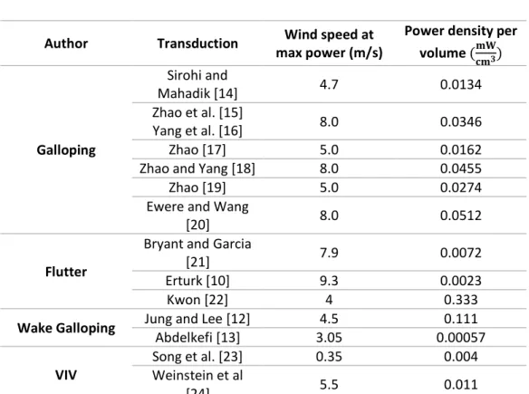
1.1.2.4 Galloping based energy harvesters

Galloping is a single degree of freedom instability in which the fluid-flow force generates an oscillation of the structure, in the perpendicular direction respect to the flow. Often this instability is the cause of the transmission line break, in presence of ice on the cable, because in normal case, with a cylindrical shape, galloping doesn’t occur. This instability happens after a certain velocity, onset speed, and it depends from the stiffness component of the system. Above the onset velocity, the system starts to increase the amplitude of the oscillation, with the same frequency of the structure. Generally, these prototypes are composed by a cantilever beam with a transducer, for example a piezoelectric patch, and a bluff body, and of course at the galloping velocity the bluff body starts to oscillate and this create a deformation on the beam, with the consequent generation of power from the transducer.

(25)

STATE OF THE ART

12

Figure 1.7 Scheme of galloping piezoelectric energy harvesting

Author Transduction Wind speed at

max power (m/s)

Power density per volume (𝐦𝐖_𝐜𝐦𝟑) Galloping Sirohi and Mahadik [14] 4.7 0.0134 Zhao et al. [15] Yang et al. [16] 8.0 0.0346 Zhao [17] 5.0 0.0162

Zhao and Yang [18] 8.0 0.0455

Zhao [19] 5.0 0.0274

Ewere and Wang

[20] 8.0 0.0512

Flutter

Bryant and Garcia

[21] 7.9 0.0072

Erturk [10] 9.3 0.0023

Kwon [22] 4 0.333

Wake Galloping Jung and Lee [12] 4.5 0.111

Abdelkefi [13] 3.05 0.00057

VIV

Song et al. [23] 0.35 0.004

Weinstein et al

[24] 5.5 0.011

Table 1.3 Comparison between different energy harvesting technology from aerodynamic instabilities

1.2 Galloping piezoelectric energy harvester

In literature it is possible to find researches about the galloping energy harvesting because, respect than vortex shedding, this source presents interesting advantages due to the self-excited and self-limiting characteristics. A first important aspect of this instability is the work range, in fact we can obtain a large wind speeds range.

A first research about galloping, using for energy harvesting, was provided by Barrero-Gil [25] modelling the system, a 1DOF model, as a simple mass-spring-damper system. In this work only a numerical solution was given, without a real design for a prototype. In order to represent the aerodynamic force, it was used a cube polynomial in

(26)

STATE OF THE ART

13 A continuum of the work was given by Sorribes-Palmer and Sanz-Andreas [26]. They obtained the aerodynamic coefficient curve directly from experimental, avoid using coefficients by literature. In this way It is possible to avoid some problems with the fitting curve, and also to obtain a correct value of the curve 𝐶𝑧 for a specific prototype.

The first study on the structure was provide by Sirohi and Mahadik. In fact in them work we can find a study on:

• A first use of two cantilever beams, instead only one, with a bluff body at the end, free to move. For this system was adopted the Rayleigh-Ritz method in order to model the coupled electromechanical effect [27];

• A piezoelectric composite beam with a bluff body, D-shape cross section, connected in parallel with the beam. In this case we can see two articular things, the first is the configuration of the prototype, because a longitudinal model, and the second is the new shape of the bluff body. An interesting result obtained in this research was that the natural frequency of the

oscillation was equal to the natural frequency of the cantilever, with a second observation about the power, because it was observed that it increased with the wind speed [14].

The influence of the bluff body shape was studied by Zhao et al [15] and Yang et al [16]. In particular they studied different type of shape, comparing experimental results for all prototypes. They studied also the effect of the aspect ratio for the rectangular shape. In Table 1.4 it is possible to see all shapes.

Section Shape Dimension h x d (mm)

40 x 40 40 x 60 40 x 26.7 40 (side) 40 (dia.)

Table 1.4 Cross sections of Yang's work [16]

From these researches was established that the best solution, in term of power, was the square section.

Using a 1DOF model it was possible to predict the power response of the system, where the aerodynamic force was modelled with a seventh order polynomial.

Another study about different bluff body shape was conducted by Abdelkefi et al. [28]. They used different shape including square, two isosceles triangles (with different base angle) and a D-section and they concluded that D-section was recommended for high wind speeds and isosceles triangle for small wind speed. They also discovered that aerodynamic coefficients are sensitive to the flow condition, laminar or turbulent.

(27)

STATE OF THE ART

14 In order to optimize a galloping energy harvesting device, Zhao et al. [29] provided a comparison of different modelling methods, trying to find advantages and

disadvantages for all.

In particular they studied a 1 DOF model, a single mode Euler-Bernoulli distributed parameter model and a multimode Euler-Bernoulli distributed parameter.

At the end they concluded that the best way in order to represent the aerodynamic force is the parameter model, instead in order to give a prediction of the cut.in wind speed, it was better to a 1 DOF model.

A problem about energy harvesting based on galloping instability is that the amplitude of oscillation can increase too much during the operational wind speeds range, with the risk of failure of the device.

In order to avoid this problem Zhao et al. [17] tried a new model that it combined an electromechanical system with a magnetic effect. This is a 2DOF model and using the electricity It is possible to change the intensity of the magnetic field, with a reduction of the amplitude oscillation at high speed.

A second method for this problem was provided by Ewere et al. [30]. They introduced a bump stop on the system in order to reduce the fatigue problem and also to reduce the amplitude oscillation with the galloping instability.

(a) (b)

(c)

Figure 1.8GPEH prototypes. (a) transversal model [15], (b) 2DOF system [29] and (c) longitudinal model [14]

(28)

STATE OF THE ART 15 Author Configuration Bluff body shape Cut-in wind speed [m/s] Bluff body dimensions [cm] Cantilever dimensions [cm] Sorohi and Mahadik [14] Longitudinal D-shape 2.5 3 in dia., 23.5 in length 9 x 3.8 x 0.0635 Zhao et al. [15] Yang et al. [16] Transversal Square 2.5 4 x 4 x 15 15 x 3.8 x 0.06 Zhao et al. [17] Transversal Square 1.0 4 x 4 x 15 17.2 x 6.6 x 0.06 Zhao and

Yang [18] Transversal Square 2.0 4 x 4 x 15 8 x 4.5 x 0.5 Zhao et al.

[19] Transversal Square 5.0 2 x 2 x 10

8.5 x 2 x 0.03 Ewere and

Wang [20] Transversal Square 8.0 5 x 5 x10

22.8 x 4 x 0.04

Table 1.5 Comparison of GPEH prototypes

1.2.1 GPEH configurations

As we just said in the previous paragraph, a galloping energy harvesting is composed by three main elements: a structure of support that is the beam, and it possible to have different material for this element, a bluff body, with a precise dimension and shape, and at the end a transducer, in our case we are interested only in piezoelectric patch.

Of course, the prototype is also composed by a clamp mechanism and an electrical circuity, and both these parameters can change the response of the system. The PZT patches are mounted on the cantilever beam, one per side, in this way we have two patches per each beam. These two patches can be connected in parallel or in series. In our case we use the series connection. The output voltage is dissipated on the resistive load, another parameter that can influence the result in term of power.

(29)

STATE OF THE ART

16 We just saw that exist two different configurations for galloping energy harvesting in literature:

• The first configuration is the transversal model, called also T-shape design. In this case the bluff body is mounted on the tip of the beam orthogonally to the beam. In this configuration we can divide in two cases, with one or two support beams. In both these models all parameters remain the same but using two beams we can avoid the moment acting on bluff body axis. Another possible advantage is that using this second model we use four PZT patches, and for this reason It is reasonable to think that the power is higher than with one beam;

• The second configuration is the longitudinal model. Here the bluff body is mounted following the beam direction. In this configuration there is only one beam and there is the possibility to reduce the length of the beam, the region without piezoelectric patch, in order to reduce the dimension of the total prototype.

(a) (b)

(c)

Figure 1.9 GPEH configurations scheme. (a) transversal one beam, (b) transversal two beams and (c) longitudinal

(30)

MATHEMATICAL MODEL

17

2 MATHEMATICAL MODEL

In this second our aim is to provide a complete mathematical model for both porotypes we want to compare at the end of this work.

We start from models we just described in the first chapter, using a general dimension for the system, because correct values we’re going to be obtain in the third chapter, after the sensitivity analysis.

Before the modelling of prototypes, we want to provide a little explanation of quasi-steady theory and assumptions of distributed parameter model, because they need for continuation.

2.1 GPEH reference layout

For application we want to study, we need to consider both configurations of energy harvester, longitudinal one and transversal. In literature there isn’t a comparison between longitudinal and transversal prototypes and with this research our purpose is to provide this comparison.

Figure 2.1 GPEH layout for a longitudinal configuration

(31)

MATHEMATICAL MODEL

18 Longitudinal layout is composed by a supporting beam structured with two

piezoelectric patches attached at each side of the beam ad a bluff body attached at the end of the beam. Bluff body can be designed with different material, in order to modify the weight, and also different dimensions, to modify the aerodynamic forces. The origin of the structure is placed on the clamped end, with the X is along the longitudinal direction and Y axis is in the oscillation direction. In Table 2.1 it is possible to find every variable used in the modal approach.

For transversal prototype we have to consider two supporting beams, instead one, with four piezoelectric patches attached. In this second configuration the bluff body is attached perpendicular to the end of both beams.

𝑋𝑖,𝑗

For the quantity named “X” the first subscript indicates the material used (“p”: piezoelectric layer, “s”: supporting beam, “b”: bluff body, “e”: extension for the bluff body). The second

subscript, if present, indicates the region in which the quantity “X” is considered

𝜙𝑗(𝑖) i-th mode of vibration for the region j

𝑉𝑖,𝑗 Volume of the material I for the region j

𝑤𝑖 Width of layer i

𝜌𝑖 Density of layer i

𝑡𝑖 Thickness of layer i

𝑚𝑖 Mass per unit length of layer i

𝐸𝑖 Young modulus of layer i

𝐿𝑗 Length of layer i

𝑑𝑖 Distance of the layer i from the neutral axis of the region j

𝐷 Side with of the bluff body

(32)

MATHEMATICAL MODEL

19

2.2 Piezoelectric beam characteristics equations

For our layout we consider a unimorph piezoelectric patch. This patch consists of a single piezoelectric layer and it is combined with different substrate able to guarantee suitable elastic properties for the patch. As we just said before, at the final prototype we use one PZT patch per each side of the beam, or beams in the transversal

configuration. In our configuration we consider the piezo patch attached at the middle of the beam.

When the beam considered is subjected to deformation, In Y direction, stress and strain for each layer vary according to the bending moment direction.

Figure 2.3 Convention for the positive direction of stress, strain and bending moment for a beam with two PZT attached to a metal beam

Piezoelectric layer produces a charge when mechanically strained. This effect is used to convert mechanical energy to electrical energy. In our case we use this effect to convert the energy introduce by aerodynamic forces, galloping instability, to electrical power. It is possible to describe this process with the constitutive equations for piezoelectric materials:

𝑆𝑖𝑗= 𝑆𝐸𝑖𝑗𝑘𝑙𝑇𝑘𝑙+ 𝑑𝑘𝑖𝑗𝐸𝑘 (2.4)

𝐷𝑗= 𝑑𝑖𝑘𝑙𝑇𝑘𝑙+ 𝜀𝑇𝑖𝑘𝐸𝑘 (2.5)

Where the mechanical strain S and stress T tensors are introduced, as well as the electric displacement D and the electric field E (the spatial directions are represented with the subscripts i, j, k, l). The other coefficients are the mechanical compliance at constant electric field 𝑆𝐸𝑖𝑗𝑘𝑙, the permittivity at constant stress 𝜀𝑇𝑖𝑘 and the coupling

matrix 𝑑𝑘𝑖𝑗. These equations compose a 3x6 matrix, made up with all piezoelectric

coefficients along different directions.

For our application the PZT patch operates only in the 3-1 mode, bending mode, meaning that the deformation in applied only at the direction 1, while the voltage is harvested along direction 3. Formulas (2.4) and (2.5) can be simply as follow:

(33)

MATHEMATICAL MODEL

20

𝑆1= 𝑆𝐸11𝑇1+ 𝑑31𝐸3 (2.6)

𝐷1= 𝑑31𝑇1+ 𝜀𝑇33𝐸3 (2.7)

And we can rearrange (2.6) and (2.7) in matrix form: [_𝐷𝑆1 3] = [ 𝑆𝐸 11 𝑑31 𝑑13 𝜀𝑇33 ] [_𝐸𝑇1 3] (2.8)

2.3 Galloping force method

The GPEH system can be seen as a single degree of freedom body, where the whole body is modelled as a concentrated mass, a spring and a damper, that represent the structural stiffness and damping capability. The aerodynamic force can be modelled as a constant flow, that hits the body surface in a normal direction. In Figure 2.4 is showed a square section bluff body subjected to aerodynamic forces. We need to consider relative velocity that is generated by the interaction between wind velocity and bluff body velocity in vertical direction.

Figure 2.4 Representation of aerodynamic forces per unit length acting on a square-section bluff body

The total aerodynamic load results along vertical direction is equal to:

𝐹𝑦= 𝐹𝐿cos 𝛼 − 𝐹𝐷sin 𝛼 (2.9)

where 𝛼 = tan−1(𝑦̇

𝑈) .

For small displacements of the angle of attack 𝛼, around the zero value and under the quasi-steady aerodynamic hypothesis, we can adopt the following simplifications:

• The relative fluid speed can be approximated as 𝑉𝑟 = √𝑈2+ 𝑦̇2≈ 𝑈2

• The angle of attack may be simplified as 𝛼 ≈ (𝑦̇ 𝑈)

(34)

MATHEMATICAL MODEL

21 • It is possible to use a first-degree Maclaurin approximation for sine and cosine:

sin 𝛼 ≈ 𝛼 and cos 𝛼 = 1

• Aerodynamic coefficients depend upon the angle of attack, so it is possible to us the Taylor’s formula as:

𝐶𝐿= 𝐶𝐿|𝛼=0+ 𝜕𝐶𝐿 𝜕𝛼|𝛼=0 𝛼 (2.10) 𝐶𝐷= 𝐶𝐷|𝛼=0+ 𝜕𝐶𝐷 𝜕𝛼|𝛼=0 𝛼 (2.11)

It can be observed that for a bluff body we have: • 𝐶𝐿|𝛼=0= 0;

• 𝜕𝐶𝐷

𝜕𝛼|_𝛼=0= 0.

Aerodynamic force along y direction can be rewrite as: 𝐹𝑦=

1 2𝜌𝐷𝐿𝑈

2_(𝐶

𝐿cos 𝛼 − 𝐶𝐷sin 𝛼) (2.12)

Considering the previous simplifications, it is possible to rewrite the force as follow: 𝐹𝑦= 1 2𝜌𝐷𝐿𝑈 2₍𝜕𝐶𝐿 𝜕𝛼|𝛼=0 − 𝐶𝐷|𝛼=0) 𝑦̇ 𝑈 (2.13)

In this linearized expression for the aerodynamic force, it is possible to express this value as an equivalent aerodynamic damping action. It can be expressed as:

𝑟𝑎𝑒𝑟𝑜 = − 1 2𝜌𝐷𝐿𝑈 ( 𝜕𝐶𝐿 𝜕𝛼|𝛼=0− 𝐶𝐷 |𝛼=0) (2.14)

Note that this contribution term can also assume a negative value and in this case if the pair of complex conjugate poles, that represent the solution of the motion

equation, are moved on the right-hand side of the imaginary plane, the equilibrium of the system will become unstable and the system will start to increase the oscillation amplitude.

In order to evaluate the condition of galloping instability acting on the system, we can observe when the total damping is negative:

(35)

MATHEMATICAL MODEL

22 If we introduce (2.14) inside the formula (2.15) it is possible to obtaing the galloping velocity: 𝑈𝑔> 𝑟𝑚𝑒𝑐ℎ −1₂𝜌𝐷𝐿𝑈 (𝜕𝐶_𝜕𝛼𝐿| 𝛼=0 − 𝐶𝐷|𝛼=0) (2.16)

At the end it is possible to show another way to express the aerodynamic force acting on the vertical direction. In fact we can interpolate the aerodynamic coefficient with a higher order polynomial in tan (α):

𝐶𝑦= ∑ 𝛼𝑖( 𝑦̇ 𝑈) 𝑖 𝑁 𝑖=1 (2.17)

Where coefficients 𝛼𝑖 are estimated from experiments, and 𝐶𝑦 takes in account drag

and lift effects. Replacing (2.17) inside (2.13) we obtain:

𝐹𝑦= 1 2𝜌𝐷𝐿𝑈 2_(𝑎 1 𝑦̇ 𝑈+ 𝑎3( 𝑦̇ 𝑈) 3 ) (2.18)

This final expression is really important for us because we will use it inside our mathematical model, whit aerodynamic coefficients from literature.

2.3.1 Influence of bluff body shape

As we have just seen, aerodynamic coefficients 𝑎1 and 𝑎3 are obtained from

experimental tests. In literature it is possible to find different values of coefficients, depending from the cross-section geometry of the bluff body.

It is important to remember that these values are valid only for small angle of attack, and them won’t still valid in big angles range. Reynolds number influences these coefficients, and for this reason in literature it is possible to find different value for different conditions. In Table 2.2 are showed different aerodynamic coefficients.

Cross-section 𝒂𝟏 𝒂𝟑 Re Source

Square 2.3 -18 33000 - 66000 Parkinson and Smith [31] Isosceles triangle (delta = 30°) 2.9 -6.2 10 5 Alonso and Meseguer [32] Isosceles triangle

(36)

MATHEMATICAL MODEL

23

D-section 1.9 6.7 104 Novak and Tanak

[34]

Table 2.2 Aerodynamic coefficients for different bluff body shape

2.4 Distributed parameter model of a GPEH

Distributed parameter model is derived by the Hamilton’s principle using Eulero-Lagrange formulation, which starts with the definition of various energy forms. The formulation is the same as the one presented in the works by Du Toit [35] and Preumont [36] and is given by the following integral:

∫ [𝛿(𝐸𝑘− 𝐸𝑝+ 𝑊𝑒) + 𝛿𝐿𝑎𝑒𝑟𝑜+ 𝛿𝐿𝑒𝑙]𝑑𝑡 = 0 𝑡2

𝑡1

(2.19) where 𝑡1 and 𝑡2 are the initial and final times, 𝐸𝑘 is the kinetic energy, 𝐸𝑝 the elastic

energy, 𝑊𝑒 is the electrical energy, 𝛿𝐿𝑎𝑒𝑟𝑜 is the work done by aerodynamic force and

𝛿𝐿𝑒𝑙 is the work done by the electric charge.

2.4.1 Assumptions

We can describe the dynamic of the GPEH using the bending vibrations of beam of continuous systems.

This model is valid under the following assumptions: 1) Small displacements;

2) Linear elastic constitutive law. Under this assumption we can consider isotropic relationship between strain and stress. This is valid in particular for metallic materials and we can consider true until the plastic yield limit is achieved;

3) Constant section and homogeneous material. For this reason, if we have different sections, we can split all of them in different regions and use the beam theory for each section. Another important concept is that all the physical properties don’t depend from the position or orientation inside the beam;

4) Damping effects are neglected;

5) No forces are applied, except at the boundaries; 6) The beam isn’t subject to tension/compression;

7) The centre of gravity of the beam is on the principal axis, for this reason the bending motion is decoupled from torsional vibrations;

8) Plane bending of the beam is studied, assuming that the plane where the bending motion occurs contains one of the principal axes of the beam section. It is easy to verify that, under this assumption, the plane bending motion

(37)

MATHEMATICAL MODEL

24 studied is totally de-coupled from a second component of bending, occurring in an orthogonal plane which contains the other principal axis of the beam section;

9) The beam is thin, the ratio between the height and length is really small, less than 1:

10) If h is the high of the section and l is the length, we must have: ℎ

𝑙 ≪ 1 (2.20)

2.4.2 Boundary conditions and stationary solutions

It is possible to define the modal equation, for every j-mode, as a combination of time and displacement. The equation is defined for each i-region of the structure:

𝑦𝑖(𝑥, 𝑡) = 𝛼𝑖𝑗(𝑥)𝛽𝑗(𝑡) (2.21)

t is referred to the time and x is referred to the distance along the structure direction,

as it is possible to see in Figure 2.5 and Figure 2.6. Instead α and β are two coefficients that we can define as:

𝛼𝑖𝑗(𝑥) = 𝐴𝑖𝑗cos 𝛾𝑥 + 𝐵𝑖𝑗sin 𝛾𝑥 + 𝐶𝑖𝑗cosh 𝛾𝑥 + 𝐷𝑖𝑗sinh 𝛾𝑥 (2.22)

𝛽𝑗(𝑡) = 𝐸𝑗cos 𝜔𝑗𝑡 + 𝐹𝑗sin 𝜔𝑗𝑡 (2.23)

Total displacement is calculated using every single displacement for each mode, so It is necessary to sum every contribute:

𝑦𝑖(𝑥, 𝑡) = ∑ 𝛼𝑖𝑗(𝑥)𝛽𝑗(𝑡) ∞

𝑗=1

(2.24)

For the present problem it is reasonable to accept an approximation and limit the summation of infinite modes to the first n modes. Depending on the range of

frequencies of interest for the problem, the model may be reduced to a three-modes or even single-mode model. For a galloping energy harvester, many authors have reported experimentally that the only significant mode is the first one [29] [27] [18]. Each domain can be considered, according to its properties, as deformable or rigid elements. For deformable sections we can use the following expression:

(38)

MATHEMATICAL MODEL

25 Instead rigid sections can be described as:

𝑦𝑖(𝑥, 𝑡) = (𝐴𝑖𝑥 + 𝐵𝑖)𝑒𝑖𝜔𝑛𝑡 (2.26)

In this project we are going to study two different layouts of prototype and for both of them we’re going to define the mathematical model. In Figure 2.5 and Figure 2.6 are showed both scheme configurations.

Figure 2.5 Transversal Model

Figure 2.6 Longitudinal Model

For longitudinal model the third region is composed by bluff body and cantilever beam, because this is the part where the bluff body attaches on the beam.

In both of models there are regions whit more the one layer, with different stiffness and density, I can use an approximation in order to compute an equivalent inertia of that region:

(39)

MATHEMATICAL MODEL 26 𝐽𝑒𝑞 = 1 𝐸𝑝 ∑ 𝐸𝑖( 𝑤𝑖𝑡𝑖3 12 + 𝑤𝑖𝑡𝑖𝑑𝑖 2₎ 𝑛 𝑖=1 (2.27)

Where 𝐸𝑝 is the Young’s modulus of the equivalent material used for the inertia

computation. In our case 𝐸𝑝 is referred to beam elastic modulus.

2.4.2.1 Transversal Model

Now It is possible to define all the formulas for each region, in order to obtain the displacement associate to the first natural mode.

𝑦1(𝑥, 𝑡) = (𝐴1cos 𝛾𝑥 + 𝐵1sin 𝛾𝑥 + 𝐶1cosh 𝛾𝑥 + 𝐷1sinh 𝛾𝑥)𝑒𝑖𝜔1𝑡 (2.28)

𝑦3(𝑥, 𝑡) = (𝐴3𝑥 + 𝐵3)𝑒𝑖𝜔1𝑡 (2.30)

From this system of equations, I can define a vector of all coefficient:

𝑥 = [ 𝐴1 𝐵1 𝐶1 𝐷1 𝐴2 𝐵2 𝐶2 𝐷2 𝐴3 𝐵3] (2.31)

It is possible to compute these coefficients using the boundary conditions. To compute these coefficients I need to obtain all the natural frequencies that I want to analyse, in our case only the first.

We have a linear system, compose by ten equations, to solve:

[𝐻]𝑥 = 0 (2.32)

Matrix H is composed by all the boundary conditions on the equilibria of

displacements and speed continuities, momentum and shear force balances between each region and considering that the first region is clamped, while the tip is a free end:

(40)

MATHEMATICAL MODEL 27 𝑦1(0, 𝑡) = 0 (2.33) 𝛿𝑦1(0, 𝑡) 𝛿𝑥 = 0 (2.34) 𝑦1(𝐿1, 𝑡) = 𝑦2(0, 𝑡) (2.35) 𝛿𝑦1(𝐿1, 𝑡) 𝛿𝑥 = 𝛿𝑦2(0, 𝑡) 𝛿𝑥 (2.36) 𝐸1𝐽1 𝛿2_𝑦 1(𝐿1, 𝑡) 𝛿𝑥2 = 𝐸2𝐽2 𝛿2_𝑦 2(0, 𝑡) 𝛿𝑥2 (2.37) 𝐸1𝐽1 𝛿3_𝑦 1(𝐿1, 𝑡) 𝛿𝑥3 = 𝐸2𝐽2 𝛿3_𝑦 2(0, 𝑡) 𝛿𝑥3 (2.38) 𝑦2(𝐿2, 𝑡) = 𝑦3(0, 𝑡) (2.39) 𝛿𝑦2(𝐿2, 𝑡) 𝛿𝑥 = 𝛿𝑦3(0, 𝑡) 𝛿𝑥 (2.40) 𝐸2𝐽2 𝛿2𝑦2(𝐿2, 𝑡) 𝛿𝑥2 + 𝑀3 𝛿2_𝑦 3(𝐿₂3, 𝑡) 𝛿𝑥2 + 𝐽3 𝛿3_𝑦 3(𝐿₂3, 𝑡) 𝛿𝑡2_𝛿𝑥 = 0 (2.41) 𝐸2𝐽2 𝛿3_𝑦 2(𝐿2, 𝑡) 𝛿𝑥23 − 𝑀3 𝛿3_𝑦 3(𝐿₂3, 𝑡) 𝛿𝑡2_𝛿𝑥 = 0 (2.42)

Now if I substitute equations (2.28), (2.29) and (2.30):

𝐴1+ 𝐶1= 0 (2.43)

𝐵1𝛾1+ 𝐷1𝛾1= 0 (2.44)

𝐴1cos(𝛾1𝐿1) + 𝐵1sin(𝛾1𝐿1) + 𝐶1cosh(𝛾1𝐿1) + 𝐷1sinh(𝛾1𝐿1)

= 𝐴2+ 𝐶2 (2.45)

−𝐴1𝛾1sin(𝛾1𝐿1) + 𝐵1𝛾1cos(𝛾1𝐿1) + 𝐶1𝛾1sinh(𝛾1𝐿1)

(41)

MATHEMATICAL MODEL 28 𝐸1𝐽1(−𝐴1𝛾12cos(𝛾1𝐿1) − 𝐵1𝛾12sin(𝛾1𝐿1) + 𝐶1𝛾12cosh(𝛾1𝐿1) + 𝐷1𝛾12sinh(𝛾1𝐿1)) = 𝐸2𝐽2(−𝐴2𝛾22+ 𝐶2𝛾22) (2.47)

𝐸1𝐽1(𝐴1𝛾13sin(𝛾1𝐿1) − 𝐵1𝛾13cos(𝛾1𝐿1) + 𝐶1𝛾13sinh(𝛾1𝐿1)

+ 𝐷1𝛾13cosh(𝛾1𝐿1)) = 𝐸2𝐽2(−𝐵2𝛾23+ 𝐷2𝛾23) (2.48)

𝐴2cos(𝛾2𝐿2) + 𝐵2sin(𝛾2𝐿2) + 𝐶2cosh(𝛾2𝐿2) + 𝐷2sinh(𝛾2𝐿2)

= 𝐵3 (2.49)

−𝐴2𝛾2sin(𝛾2𝐿2) + 𝐵2𝛾2cos(𝛾2𝐿2) + 𝐶2𝛾2sinh(𝛾2𝐿2)

+ 𝐷2𝛾2 cosh(𝛾2𝐿2) = 𝐴3 (2.50) 𝐸2𝐽2(−𝐴2𝛾22cos(𝛾2𝐿2) − 𝐵2𝛾22sin(𝛾2𝐿2) + 𝐶2 𝛾22cosh(𝛾2𝐿2) + 𝐷2 𝛾22sinh(𝛾2𝐿2)) + 𝑀3[−𝜔𝑛2 𝐿3 2 (𝐴3 𝐿3 2 + 𝐵3)] − 𝐽3𝜔𝑛2𝐴3= 0 (2.51)

𝐸2𝐽2(𝐴2𝛾23sin(𝛾2𝐿2) − 𝐵2𝛾23cos(𝛾2𝐿2) + 𝐶2𝛾23sinh(𝛾2𝐿2)

+ 𝐷2𝛾23cosh(𝛾2𝐿2)) + 𝑀3𝜔𝑛2𝐴3 𝐿3 2 + 𝑀3𝜔𝑛 2_𝐵 3 = 0 (2.52)

In the next page It is possible to see the matrix H that I can obtain from this system of equations.

(42)

MATHEMATICAL MODEL

(43)

MATHEMATICAL MODEL

30 2.4.2.2 Transversal Model

For the longitudinal prototype we saw that there are to consider four regions instead three:

𝑦4(𝑥, 𝑡) = (𝐴4𝑥 + 𝐵4)𝑒𝑖𝜔1𝑡 (2.56)

Like for the transversal model we’re going to define a vector with all the coefficients:

𝑥 = [ 𝐴1 𝐵1 𝐶1 𝐷1 𝐴2 𝐵2 𝐶2 𝐷2 𝐴3 𝐵3 𝐶3 𝐷3 𝐴4 𝐵4] (2.57)

As for the transversal prototype we have to rewrite the boundary conditions:

𝑦1(0, 𝑡) = 0 (2.58) 𝛿𝑦1(0, 𝑡) 𝛿𝑥 = 0 (2.59) 𝑦1(𝐿1, 𝑡) = 𝑦2(0, 𝑡) (2.60) 𝛿𝑦1(𝐿1, 𝑡) 𝛿𝑥 = 𝛿𝑦2(0, 𝑡) 𝛿𝑥 (2.61) 𝐸1𝐽1 𝛿2_𝑦 1(𝐿1, 𝑡) 𝛿𝑥2 = 𝐸2𝐽2 𝛿2_𝑦 2(0, 𝑡) 𝛿𝑥2 (2.62)

(44)

MATHEMATICAL MODEL 31 𝐸1𝐽1 𝛿3_𝑦 1(𝐿1, 𝑡) 𝛿𝑥3 = 𝐸2𝐽2 𝛿3_𝑦 2(0, 𝑡) 𝛿𝑥3 (2.63) 𝑦2(𝐿2, 𝑡) = 𝑦3(0, 𝑡) (2.64) 𝛿𝑦2(𝐿2, 𝑡) 𝛿𝑥 = 𝛿𝑦3(0, 𝑡) 𝛿𝑥 (2.65) 𝐸2𝐽2 𝛿2𝑦2(𝐿2, 𝑡) 𝛿𝑥2 = 𝐸3𝐽3 𝛿2𝑦3(0, 𝑡) 𝛿𝑥2 (2.66) 𝐸2𝐽2 𝛿3_𝑦 2(𝐿2, 𝑡) 𝛿𝑥3 = 𝐸3𝐽3 𝛿3_𝑦 3(0, 𝑡) 𝛿𝑥3 (2.67) 𝑦3(𝐿3, 𝑡) = 𝑦4(0, 𝑡) (2.68) 𝛿𝑦3(𝐿3, 𝑡) 𝛿𝑥 = 𝛿𝑦4(0, 𝑡) 𝛿𝑥 (2.69) 𝐸3𝐽3 𝛿2𝑦3(𝐿3, 𝑡) 𝛿𝑥2 + 𝑀4 𝛿2𝑦4(𝐿₂4, 𝑡) 𝛿𝑥2 + 𝐽4 𝛿3𝑦4(𝐿₂4, 𝑡) 𝛿𝑡2_𝛿𝑥 = 0 (2.70) 𝐸3𝐽3 𝛿3𝑦3(𝐿3, 𝑡) 𝛿𝑥23 − 𝑀4 𝛿3𝑦4(𝐿₂4, 𝑡) 𝛿𝑡2_𝛿𝑥 = 0 (2.71)

Without substitute equations inside the boundary conditions, it is possible to write the matrix H.

(45)

MATHEMATICAL MODEL

(46)

MATHEMATICAL MODEL

33

2.4.3 Kinetic energy

In order to define the modal mass, we can use the kinetic energy 𝐸𝑘. This is written as

the sum of every mass contribution from different regions. We must define modal mass for both prototypes.

2.4.3.1 Transversal model

From the previous consideration, we just know that GPEH is composed by three regions: 𝐸𝑘 = 1 2 ∫ 𝑦̇1 𝑇_𝜌 𝑠𝑦̇1𝑑𝑉 𝑉𝑠1 + 21 2 ∫ 𝑦̇1 𝑇_𝜌 𝑝𝑦̇1𝑑𝑉 𝑉𝑝1 +1 2 ∫ 𝑦̇2 𝑇_𝜌 𝑠𝑦̇2𝑑𝑉 𝑉𝑠2 +1 2 ∫ 𝑦̇3 𝑇_𝜌 𝑏𝑦̇3𝑑𝑉 𝑉𝑏3 (2.72)

With subscripts s, p and b we refer to beam, piezo and bluff body.

Because the structure is symmetric, we can double the contribution. Now it is possible to introduce the modal approach, using only the first natural mode, according to the previous assumption:

𝑦𝑖 = 𝜙𝑖(1)𝑞(1) where 𝜙𝑖(1)= 𝜙𝑖(1)(𝑥𝑖) (2.73)

And deriving:

𝑦𝑖̇ = 𝜙𝑖(1)𝑞̇(1) (2.74)

So now we are going to substitute this equation inside the kinetic energy.

We can also simplify the volume integrals because the quantities have to be integrated only along the axial coordinate, and we obtain the following form:

𝐸𝑘 = 1 2[𝑤𝑠𝑡𝑠𝜌𝑠∫ 𝜙1 2_𝑑𝑥 1 𝐿1 0 + 2𝑤𝑝𝑡𝑝𝜌𝑝∫ 𝜙12𝑑𝑥1 𝐿1 0 + 𝑤𝑠𝑡𝑠𝜌𝑠∫ 𝜙22𝑑𝑥2 𝐿2 0 + 𝑤𝑏𝑡𝑏𝜌𝑏∫ 𝜙32𝑑𝑥3 𝐿3 0 ] 𝑞̇2 =1 2𝑀 ∗_𝑞̇2 (2.75)

(47)

MATHEMATICAL MODEL

34 At the end from the last equation we can define the modal mass:

𝑀∗_{= 𝑤} 𝑠𝑡𝑠𝜌𝑠∫ 𝜙12𝑑𝑥1 𝐿1 0 + 2𝑤𝑝𝑡𝑝𝜌𝑝∫ 𝜙12𝑑𝑥1 𝐿1 0 + 𝑤𝑠𝑡𝑠𝜌𝑠∫ 𝜙22𝑑𝑥2 𝐿2 0 + 𝑤𝑏𝑡𝑏𝜌𝑏∫ 𝜙32𝑑𝑥3 𝐿3 0 (2.76)

The overall kinetic energy is therefore: 𝐸𝑘 =

1 2𝑀

∗_𝑞̇2 _(2.77)

By differentiating this equation with respect to the derivative of the modal coordinate

q it is obtained:

𝐸𝑘 = 𝛿𝑞̇𝑀∗𝑞̇ (2.78)

2.4.3.2 Longitudinal model

Now for this second prototype the only different is about the number of the regions that I’ve to consider. Indeed, as already discussed, now we’ve four regions, instead three: 𝐸𝑘 = 1 2 ∫ 𝑦̇1 𝑇_𝜌 𝑠𝑦̇1𝑑𝑉 𝑉𝑠1 + 21 2 ∫ 𝑦̇1 𝑇_𝜌 𝑝𝑦̇1𝑑𝑉 𝑉𝑝1 +1 2 ∫ 𝑦̇2 𝑇_𝜌 𝑠𝑦̇2𝑑𝑉 𝑉𝑠2 +1 2 ∫ 𝑦̇3 𝑇_𝜌 𝑠𝑦̇3𝑑𝑉 𝑉𝑠3 +1 2 ∫ 𝑦̇3 𝑇_𝜌 𝑏𝑦̇3𝑑𝑉 𝑉𝑏3 +1 2 ∫ 𝑦̇4 𝑇_𝜌 𝑏𝑦̇4𝑑𝑉 𝑉𝑏4 (2.79)

Without rewrite every step, the modal mass is defined as follow: 𝑀∗= 𝑤𝑠𝑡𝑠𝜌𝑠∫ 𝜙12𝑑𝑥1 𝐿1 0 + 2𝑤𝑝𝑡𝑝𝜌𝑝∫ 𝜙12𝑑𝑥1 𝐿1 0 + 𝑤𝑠𝑡𝑠𝜌𝑠∫ 𝜙22𝑑𝑥2 𝐿2 0 + 𝑤𝑠𝑡𝑠𝜌𝑠∫ 𝜙32𝑑𝑥3 𝐿3 0 + 𝑤𝑏𝑡𝑏𝜌𝑏∫ 𝜙32𝑑𝑥3 𝐿3 0 + 𝑤𝑏𝑡𝑏𝜌𝑏∫ 𝜙42𝑑𝑥4 𝐿4 0 (2.80)

(48)

MATHEMATICAL MODEL

35 By differentiating this equation with respect to the derivative of the modal coordinate

q it is obtained:

𝐸𝑘 = 𝛿𝑞̇𝑀∗𝑞̇ (2.81)

2.4.4 Elastic energy

The elastic energy is determined by the sum of strain and stress deformations that the GPEH experiences. For this reason, since the fourth region is not deformable it will not be included in the following definition of the total elastic energy:

𝐸𝑝= 1 2 ∫ 𝑆 𝑇 𝑠1𝑇𝑠1𝑑𝑉𝑠1 𝑉𝑠1 + 2 ∫ 𝑆𝑇𝑝1𝑇𝑝1𝑑𝑉𝑝1 𝑉𝑠1 +1 2 ∫ 𝑆 𝑇 𝑠2𝑇𝑠2𝑑𝑉𝑠2 𝑉𝑠2 +1 2 ∫ 𝑆 𝑇 𝑠3𝑇𝑠3𝑑𝑉𝑠3 𝑉𝑠3 +1 2 ∫ 𝑆 𝑇 𝑏3𝑇𝑏3𝑑𝑉𝑏3 𝑉𝑠1 (2.82)

Then the formula is re-arranged by substituting the following definitions that apply respectively for stress and strain:

𝑆 = −𝑧𝛿

2_𝑦

𝛿𝑥2 (2.83)

𝑇 = 𝑐𝑆 (2.84)

According to the piezoelectric constitutive law it is possible to state:

𝑇𝑝1 = 𝑐𝐸11𝑆𝑝1− 𝑒31𝐸3 (2.85)

The overall elastic energy can be split in the electrical contribution, it is given by the piezoelectric patch, and contribution to the other layers.

𝐸_{𝑝𝑝𝑧𝑡} = ∫ 𝑧2(𝛿 2_𝑦 𝛿𝑥2) 2 𝑐𝐸11𝑑𝑉𝑝 𝑉𝑝 + ∫ 𝑧2𝛿 2_𝑦 𝛿𝑥2𝑒31𝐸3𝑑𝑉𝑝 𝑉𝑝 (2.86)

The connection for our prototypes is the series connection. The value 𝑒31 has opposite

sign for the top and bottom PZT layers, and electric fields are: 𝐸3 = −

𝑉𝑠

2𝑡𝑝 (2.87)

(49)

MATHEMATICAL MODEL

36 Considering that in equation (2.86)the quantities width of cross-section, elastic modulus and electric field are constant for any location of the volume, integrals can be simplified as: 𝐸_{𝑝𝑝𝑧𝑡} = 𝑤𝑝𝑐𝐸11∫ ( 𝛿2𝑦 𝛿𝑥2) 2 ∫ 𝑧2_{𝑑𝑧𝑑𝑥} 1 ℎ_{𝑝+𝑡𝑝} ℎ𝑝 𝐿1 0 + 𝑒31 𝑉𝑠 2𝑡𝑝 𝑤𝑝∫ 𝛿2_𝑦 𝛿𝑥2∫ 𝑧𝑑𝑧𝑑𝑥1 ℎ_{𝑝+𝑡𝑝} ℎ𝑝 𝐿1 0 (2.88)

The integrals on the z axis are then solved:

𝐸_{𝑝𝑝𝑧𝑡} = 𝑤𝑝𝑐𝐸11∫ ( 𝛿2𝑦 𝛿𝑥2) 2 1 3[(ℎ𝑝+ 𝑡𝑝) 3 − (ℎ𝑝) 3 ] 𝑑𝑥1 𝐿1 0 + 𝑒31 𝑉𝑠 2𝑡𝑝 𝑤𝑝∫ 𝛿2_𝑦 𝛿𝑥2 𝐿₁ 0 1 2[(ℎ𝑝+ 𝑡𝑝) 2 − (ℎ𝑝) 2 ] (2.89)

Solving the axial integration, it is found:

𝐸_{𝑝𝑝𝑧𝑡} = 𝑤𝑝𝑐𝐸11 1 3[(ℎ𝑝+ 𝑡𝑝) 3 − (ℎ𝑝) 3 ] ∫ 𝜙1′′(1)2𝑑𝑥 𝑞2 𝐿1 0 +1 2𝑒31 𝑉𝑠 2𝑡𝑝 𝑤𝑝[𝑡𝑝2+ 2𝑡𝑝ℎ𝑝][𝜙1′(1)(𝐿1) − 𝜙1′(1)(0)]𝑞 (2.90)

The variable 𝜃𝑠 is then introduced as:

𝜃𝑠= 𝑒31

𝑤𝑝

2 (𝑡𝑝+ 2ℎ𝑝) (2.91)

Come back to the definition of elastic energy, the rest of integrals can be solved in a similar way: