Brain magnetic resonance imaging generation using generative adversarial networks

(1)

Politecnico di Milano

SCHOOL OF INDUSTRIAL AND INFORMATION ENGINEERING Master of Science in Computer Science and Engineering

Brain Magnetic Resonance Imaging

Generation using Generative

Adversarial Networks

Supervisor Daniele LOIACONO Co-Supervisor Edoardo GIACOMELLO Candidate Emanuel ALOGNA – 893592 Academic Year 2018 – 2019

(2)

(3)

To the ones that never stop believing in themselves. To the fools who always dream.

(4)

(5)

Ringraziamenti

Prima di tutto vorrei ringraziare il Prof. Daniele Loiacono, mio relatore e guida in questo percorso non privo di difficoltà, e il Dott. Edoardo Giacomello per la loro grande disponibilità durante questi mesi di lavoro ma anche per la pazienza mostrata, il continuo supporto, gli spunti fondamentali e i confronti costruttivi che mi hanno permesso di realizzare questa tesi. Grazie per avermi stimolato e permesso di appassionarmi ancora di più a questa materia.

Grazie a mia mamma e mio papà, che non hanno mai smesso di incoraggiarmi e mi hanno supportato (e sopportato) in ogni modo possibile durante questi anni, permettendomi di concentrarmi sullo studio a tempo pieno e dandomi la possibilità di vivere una bellissima esperienza all’estero. Tutto questo, senza di loro, non sarebbe stato possibile.

Un ringraziamento speciale ai miei fratelli che mi spingono a mettermi sempre in gioco: a Dani, la persona con la quale ho sempre potuto parlare di qualsiasi cosa, e a Mirko che, nonostante la distanza, non ha mai fatto mancare i suoi preziosi consigli. Grazie a Simona, che ormai è come una sorella, e grazie a nonna Uccia, che aspettava

più di chiunque altro questo momento.

Ringrazio Liuch, collega nonchè uno dei miei migliori amici, con cui ho avuto la fortuna di condividere questi cinque anni universitari, un progetto dopo l’altro, esame dopo esame. Finalmente siamo riusciti a tagliare questo traguardo.

Un grazie speciale anche a Ippo, Rich, Erik e Barte per esserci sempre stati, anche nei momenti difficili. Amici di una vita, con cui spero di condividere ancora tanti momenti come questo.

Desidero inoltre ringraziare Lollo e Lello, compagni di studio in biblioteca fino a tarda notte, e grazie a Gio, per le domeniche passate in aula studio sin dalla mattina e per le sciate in montagna in uno dei momenti di maggiore stress di questi mesi. Grazie infine a Salva, Dave, Mutto e Fabio che, tra calcetti e pause in biblioteca, hanno reso più leggeri gli ultimi anni di questo viaggio.

(6)

(7)

List of Figures

Figure 2.1 Pix2Pix example from Isola et al. . . 22

Figure 2.2 Generative Adversarial Network Framework . . . 24

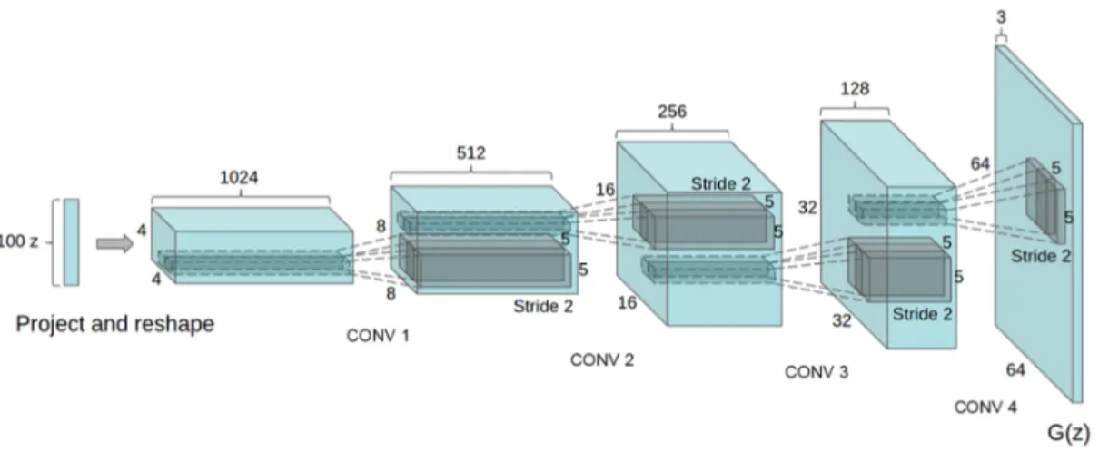
Figure 2.3 Layers from DCGAN, Radford, Metz, and Chintala . . . 26

Figure 2.4 Samples from Pix2Pix, Isola et al. . . 27

Figure 2.5 Generator architectures in Pix2Pix network . . . 29

Figure 2.6 Patch size variations in PatchGAN discriminator . . . 29

Figure 3.1 Brain MRI sequences from BRATS2015: T2 and T2flair . . . 32

Figure 3.2 T1c slice in HG and LG subjects . . . 34

Figure 3.3 Data distribution by set and tumor grade . . . 35

Figure 3.4 The four MRI sequences: T1, T2, T1c, T2flair . . . 37

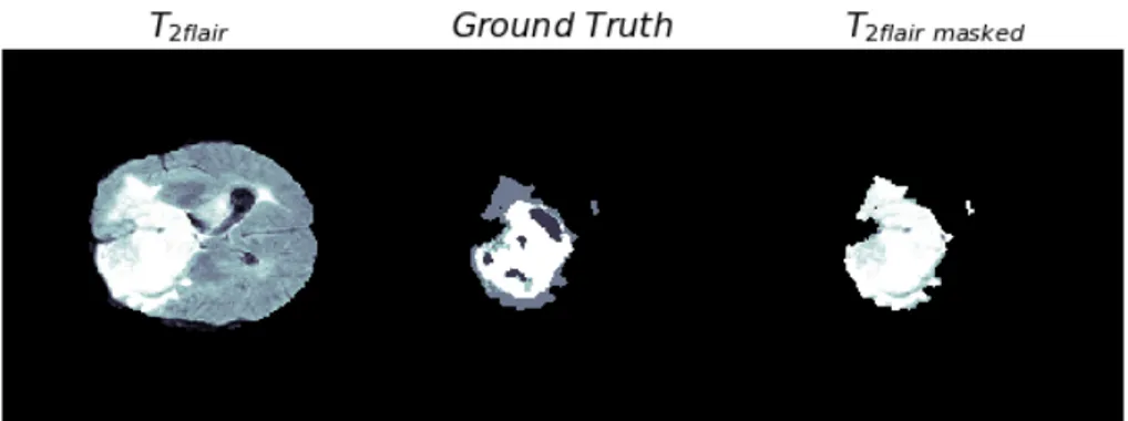
Figure 3.5 GT used as mask to segment the T2flair tumor area . . . 38

Figure 3.6 An example of consecutive T2 slices extracted from a volume . 39 Figure 4.1 A batch from training set: 32 T1 processed slices . . . 45

Figure 4.2 Generator architecture from pix2pix . . . 46

Figure 4.3 Discriminator architecture from pix2pix . . . 48

Figure 4.4 Generator architecture from MI-pix2pix . . . 50

Figure 4.5 Discriminator architecture from MI-pix2pix . . . 50

Figure 4.6 Generator architecture of MI-GAN . . . 52

Figure 4.7 Discriminator architecture of MI-GAN . . . 54

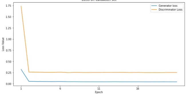
Figure 4.8 Validation loss during MI-GAN training . . . 56

Figure 4.9 T1c predictions from MI-GAN . . . 57

Figure 4.10 T 2 slice before and after crop to 155x194 . . . 59

Figure 4.11 T2f lair slices masked with the ground truth . . . 62

Figure 4.12 Comparison between Ground Truths and Segmentations . . . 64

Figure 5.1 P2P(T2→1) and P2P(T1c→1) predictions . . . 69

Figure 5.2 P2P(T1→2) and P2P(T2f lair→2) predictions . . . 69

Figure 5.3 Qualitative results from the generation of T1 . . . 70

Figure 5.4 Qualitative results from the generation of T2 . . . 71

Figure 5.5 Qualitative results from the generation of T1c. . . 72

Figure 5.6 Qualitative results from the generation of T2f lair . . . 73

Figure 5.7 Segmentations using GAN predictions . . . 74

Figure 6.1 Configuration example in Skip Connections Analysis . . . 80

Figure 6.2 Qualitative results from turning off the skips in MI-pix2pix . . 81

Figure 6.3 Qualitative results from skips perturbation in MI-pix2pix . . . 82

(10)

Figure 6.5 Qualitative results from internal connections off in MI-pix2pix 83 Figure 6.6 Percentual degradation in the performances of MI-pix2pix . . 85 Figure 6.7 Percentual degradation in the performances of different models 86 Figure A.1 Qualitative results from turning off the skips in pix2pix . . . . 100 Figure A.2 Qualitative results from turning off the skips in MI-GAN . . . 101 Figure A.3 Qualitative results from skips perturbation in pix2pix . . . 102 Figure A.4 Qualitative results from skips perturbation in MI-GAN . . . . 103 Figure A.5 Qualitative results from internal connections off in pix2pix . . 104 Figure A.6 Qualitative results from internal connections off in MI-GAN . 105

(11)

List of Tables

Table 3.1 Values from different volumes before normalization . . . 41

Table 3.2 Values from different volumes after normalization . . . 41

Table 4.1 Train time/epoch of pix2pix using a reduced set of 1024 images 44 Table 4.2 Generators input and output shapes used during training . . . 58

Table 4.3 Discriminators input and output shapes used during training . 58 Table 5.1 Generation of T1: performances on the test set . . . 66

Table 5.2 Generation of T2: performances on the test set . . . 67

Table 5.3 Generation of T1c: performances on the test set . . . 67

Table 5.4 Generation of T2f lair: performances on the test set . . . 68

Table 5.5 Segmentation performances (on test set) using T2f lair predictions 68 Table 5.6 Training time (in epochs) of every model . . . 68

Table 6.1 Quantitative results from turning off the skips in MI-pix2pix . 80 Table 6.2 Quantitative results from skips perturbation in MI-pix2pix . . . 81

Table 6.3 Quantitative results from internal connections off in MI-pix2pix 83 Table A.1 Quantitative results from turning off the skips in pix2pix . . . . 100

Table A.2 Quantitative results from turning off the skips in MI-GAN . . . 101

Table A.3 Quantitative results from skips perturbation in pix2pix . . . 102

Table A.4 Quantitative results from skips perturbation in MI-GAN . . . . 103

Table A.5 Quantitative results from internal connections off in pix2pix . . 104 Table A.6 Quantitative results from internal connections off in MI-GAN . 105

(12)

(13)

Abstract

Magnetic Resonance Imaging (MRI) is nowadays one of the most common medical imaging techniques, due to the non-invasive nature of this type of scan that can acquire many modalities (or sequences), each one with a different image appearance and unique insights about a particular disease. However, it is not always possible to obtain all the sequences required, due to many issues such as prohibitive scan times or allergies to contrast agents. To overcome this problem and thanks to the recent improvements in Deep Learning, in the last few years researchers have been studying the applicability of Generative Adversarial Network (GAN) to synthesize the missing modalities. Our work proposes a detailed study that aims to demonstrate the power of GANs in generating realistic MRI scans of brain tumors through the implementation of different models. We trained in particular two kind of networks which differ from the number of sequences received in input, using a dataset composed by 274 different volumes from subjects with brain tumor, and, among a set of different evaluation metrics implemented to test our results, we validated the quality of the predicted images using also a segmentation model. In addition, we analysed the GANs trained by performing some experiments to understand how the information passes through the generator network. Our results show that the synthesized sequences are highly accurate, realistic and in some cases indistinguishable from true brain slices of the dataset, highlighting the advantage of multi-modal models that, compared to the unimodal ones, can exploit the correlation between available sequences. Moreover, they demonstrate the effectiveness of skip connections and their crucial role in the generative process by showing the significant degradation in the performances, analysed in both a qualitative and quantitative way, when these channels are turned off or perturbed.

(14)

(15)

Estratto in lingua Italiana

L’imaging a risonanza magnetica (MRI) è oggi una delle più comuni tecniche di generazione di immagini mediche, per via della natura non invasiva di questo tipo di scansione che permette di acquisire varie modalità (o sequenze) della parte del corpo scansionata, ognuna diversa dall’altra per livello di risoluzione e contrasto utilizzato. Tuttavia, non è sempre possibile ottenere tutte le sequenze richieste, a causa di molteplici problemi, tra cui i tempi di scansione proibitivi o le allergie dei pazienti agli agenti di contrasto. Per ovviare a questo problema e grazie ai recenti miglioramenti nel campo del Deep Learning, negli ultimi anni i ricercatori hanno studiato l’applicabilità delle Reti Antagoniste Generative (GAN) alla generazione delle modalità mancanti. Il nostro lavoro propone uno studio dettagliato che mira a dimostrare l’abilità delle GAN nel generare scansioni MRI realistiche di tumori cerebrali attraverso l’implementazione di diversi modelli. Abbiamo allenato in particolare due tipi di reti che differiscono per il numero di sequenze ricevute in input, utilizzando un dataset composto da 274 diversi volumi appartenenti a pazienti con tumori cerebrali e, tra una serie di diverse metriche implementate per valutare i nostri risultati, abbiamo validato la qualità dell’immagine generata dalla rete usando anche un modello di segmentazione. Inoltre, abbiamo analizzato le GAN addestrate, eseguendo alcuni esperimenti per capire come il contenuto informativo ricevuto in input passi attraverso il generatore, ovvero una delle due reti neurali che compongono una GAN. I nostri risultati dimostrano che le sequenze sintetizzate sono altamente accurate, realistiche e in alcuni casi indistinguibili dalle immagini provenienti dal dataset, evidenziando il vantaggio dei modelli multi-input che, rispetto a quelli single-multi-input, possono sfruttare la correlazione presente tra le sequenze che sono disponibili. Inoltre, dimostrano l’efficacia delle skip connections e il loro ruolo fondamentale nel processo generativo mostrando come, spegnendo o perturbando i canali, le prestazioni della rete subiscano un calo significativo.

(16)

(17)

Chapter 1 Introduction

Medical imaging is crucial for clinical analysis and medical intervention since it gives important insights about some diseases whose structures might be hidden by the skin or by the bones. One of the most common techniques used nowadays is the Magnetic Resonance Imaging ( MRI), ubiquitous in hospitals and medical centers, first because of its non-invasive nature, since, differently from other imaging technologies, doesn’t make use of X-ray radiography and secondly because of the recent improvements in the software and hardware instrumentation used. In this type of imaging, various sequences (or modalities) can be acquired and each sequence can give useful and different insights about a particular problem of the patient. For example the T1-weighted sequence can

distinguish between gray and white matter tissues while T2-weighted is more indicated

to highlight fluid from cortical issue.

The problem about MRI is that sometimes there isn’t the possibility to acquire all the sequences that would be required in order to diagnose a disease and this is due to different reasons: sometimes there isn’t enough time to collect all the needed sequences, sometimes it’s too expensive to acquire all of them. Furthermore, missing sequences might occur because of allergies in the patient that don’t allow to obtain modalities where an exogenous contrast agent, a substance useful to increase the contrast between structures or fluids within the target area, is used to make the image clearer. It can also happen that, for a given patient, some scans might be unusable due to the presence of errors, corruptions or machine settings not defined in the proper way [1].

It would be useful, then, to find a way to generate a prediction of the missing sequences by using the modalities already acquired for a given patient. These generated predictions then could be used either as direct aid to the doctor that has to make a diagnosis for a patient that maybe can’t have injected into his body any kind of

(18)

contrast agent, or could be used as one of the input pieces of a bigger pipeline. Thanks to the recent improvements in Machine Learning, but more in particular in the Deep Learning (DL) field, the generation of missing modalities has become an objective feasible to reach, both in terms of efficiency of the obtained result and in terms of time spent in order to reach something meaningful.

In the last few years interest toward Machine Learning and Deep Learning has grown exponentially: just to give an idea to the incredible spread that is having this Artificial Intelligence (AI) research area, in the 2016 and 2017 over 400 contribu-tions related to Deep Learning applied to Medical Image Analysis were published [2]. It has been shown that DL has been able to reach very competitive results in many medical task: classification, detection, segmentation, registration of different areas and structures within the human body. Many progresses have been done and further are yet to come in order to reach results as accurate and precise as possible in crucial applications such as cancer cell classification, lesion detection, organ segmentation and image enhancement [3].

The most successful DL architecture in medical image analysis is the Convolutional Neural Network (CNN): a neural network with multiple hidden layers between the input and the output layers. The initial problem with this type of architecture was that researchers weren’t able to train these deep neural networks in an efficient way. A breakthrough was the work described in [4] that represents a huge contribution to the field since the proposed CNN, called AlexNet, won the ImageNet competition in 2012 by a large margin. The peculiarity of AlexNet was that its competitive results and high performances were obtained in relative short time, due to the fact that the designer of this network made the training feasible by the utilization of a Graphics processing unit (GPU).

Another important breakthrough in the field was represented by the introduction of Generative Adversarial Networks, a class of machine learning systems invented by Ian J. GoodFellow in 2014 [5] that we used in this work to solve the problem of missing modalities.

1.1 Scope

In this work we study the applicability of Generative Adversarial Networks to the domain of medical imaging, by focusing on the generation of brain MRI sequences

(19)

1.2. Thesis Structure

in order to overcome the problem of missing or unusable modalities and so to avoid repeating the exams multiple times. In particular, we propose a detailed study on the predictive power of three different GAN implemented: the first one is a unimodal model proposed by Isola et al. and called pix2pix [6], while the other two networks are MI-pix2pix, a multi-input version of pix2pix, and MI-GAN, a modified version of the MM-GAN proposed by Sharma et al. in [1], adapted to the multi-input single-output scenario.

We evaluate, then, the results obtained from the trained networks by assessing the performances in both a qualitative way, so with human perception, and a quantitative way, through different metrics implemented to test the generated quality of the tumor area, that needs to be synthesized with high accuracy, as well as the overall quality of the whole image.

Moreover, for studying the capabilities of the network and how skip connections affect the generative process, we show how much the performances can deteriorate by switching off or perturbing the channels in the generator network.

The two main contributions of this work can be summarized as follows:

• We define and compare two multi-modal GANs, MI-pix2pix and MI-GAN, that receive the same number of inputs but have different architectures and use different loss functions.

• We present a systematic analysis of skip connections that extends the analysis of the generator architecture in [6].

1.2 Thesis Structure

In Chapter 2 we present the related work and the theoretical background needed to make more understandable the work discussed in the following chapters. Chapter 3 describes in detail the dataset used and how it has been preprocessed in order to make it work with our models. In Chapter 4 we present to the reader the neural network architecture implemented, along with the training algorithm and the metrics that we decided to use in order to evaluate, quantitatively, the results obtained, that are presented in Chapter 5. In Chapter 6 further experiments on our trained models are described. Finally, Chapter 7 contains our general considerations about this work, a description of the open problems related to the topic and a discussion on possible applications and future develops.

(20)

(21)

Chapter 2 State of the Art

In this chapter we first present the related work on the Generative Adversarial Networks in the literature (2.1) and then, in Section 2.2, we introduce the theoretical aspects our work is based upon, while giving the reader an overview of the tools and techniques we applied in our models, in order to better understand the setting in which our work takes place.

2.1 Related Work

GANs have been used in many data domains, but the images one is where this type of neural network obtained the most significant results so far. In [5] this architecture has been tested for the first time on a range of image datasets including MNIST [7], the Toronto Face Database [8] and CIFAR-10 [9]. Isola et al. applied GANs to the image-to-image translation task and, in order to explore the generality of their work [6], experimented with a variety of settings and datasets such as generating the night version of an image whose daily version was given as input to the network or synthesizing the picture of a building by only observing its relative architecture label as input after a training performed on CMP Facades (Figure 2.1).

2.1.1 GANs in Medical Imaging

Countless studies about medical image synthesis were approached using GANs. In particular, cross modality image synthesis (so the conversion of the input image of one modality to the output of another modality) is the most important application of this architecture: in 2018, was even published a review [2] about all the work and progresses that have been done in the field of medical imaging through the application of GANs. The authors described the magnetic resonance as the most common imaging modality explored in the literature related to this generative approach invented by Goodfellow

(22)

Figure 2.1. Examples of image-to-image translation from the work of Isola et al. [6]

and this is probably due to the fact that GANs, through the cross modality synthesis, can reduce the excessive amount of time requested from Magnetic Resonance (MR) acquisition.

Many different approaches and datasets have been used in the literature in order to overcome the problem of missing modalities. Orbes-Arteaga et al., in [10], since most of the datasets contain only T1 or T1/T2/PD scans due to logistical reasons,

implemented a GAN that generates T2f lair of the brain using T1 modality. In [11],

Camileri et al. developed a variant of the original GAN, called Laplacian pyramid framework (LAPGAN) that synthesizes images in a coarse-to-fine way. This method, as the name suggests, is based on Laplacian pyramid and allows to generate initially an image with low resolution and then, incrementally, add details to it. Another approach to generate missing modalities was proposed in [12] where they presented two possible scenarios, based on the given dataset: they use a model called pGAN (that incorporates a pixel-wise loss into the objective function) when the multi-contrast images are spatially registered while they adopt a cycleGAN [13] in the more realistic scenario in which pixels are not aligned between contrasts. A cycleGAN is a GAN variant characterized by the fact that has two generators, two discriminators and uses a cycle consistency loss with a collection of training images from the source and target domain that don’t need to be related in any way.

Most of the papers about Generative Adversarial Networks, and also this work, though, are based on a training performed using paired examples, with input image and target image perfectly aligned.

It is worth to cite also the work done by Anmol Sharma and Ghassan Hamarneh that were, to the best of their knowledge [1], the first to propose a many to many generative model, capable of synthesize multiple missing sequences given a combination

(23)

2.2. Theoretical Background

of various input sequences. Furthermore, they were the first to apply the concept of curriculum learning, based on the variation of the difficulty of the examples that are shown during the network training.

MRI isn’t the only imaging technique where GAN has been applied to: in litera-ture is possible to find various publications of generative models that use Positron Emission Tomography (PET), Computerized Tomography (CT) or Magnetic Reso-nance Angiohraphy (MRA) images. Olut et al., in 2018, demonstrated that GAN works efficiently even when the source imaging technique is different from the target one: they were the first ones to synthesize MRA brain images from T1 and T2 MRI

modalities [14]. Ben-Cohen et al. published in the same year an article [15] explaining how to generate PET images using CT scans through a fully connected neural network, whose output is improved and refined by a conditional GAN (cGAN) [16].

The work related to the generation of medical image is huge and new papers about the topic are being published every week. Many approaches have been already tested and many datasets have been used but there are still lots of challenges that need to be solved in order to be able to be employed in medical imaging [2] and since there is still room for improvements in the application of generative models in medical imaging, we present in this work a complete study on different architectures of GAN used to generate missing modalities of brain scans, followed by an analysis of the information that passes through the inner channels and through the skip connections of the generator networks.

2.2 Theoretical Background

The architecture of the main model used in our work, the Generative Adversarial Network, is based on the Convolutional Neural Network: a deep neural network with many hidden layers that nowadays is proved successful in many application going from Image Recognition to Video Analysis, passing through Natural Language Processing, Anomaly detection, Drug Discovery, etc.

2.2.1 Convolutional Neural Network

The 1980, period in which David H. Hubel and Torsten Wiesel gave crucial insights about the structure of the visual cortex (the researchers are winners of the 1981 Nobel Price in Physiology or Medicine for their work), is the starting point from which convolutional neural networks started to gradually evolve into what is today

(24)

the architecture most used in DL.

The milestone is represented by the work of Yann LeCun that in 1998 developed a model, LeNet-5, to identify handwritten digits for zip code recognition in the postal service [7]. This model was composed by traditional building blocks such as fully connected layers and sigmoid activation functions but also by convolutional layers and pooling layers, introduced for the first time.

The most important building block is the convolutional layer, based on the mathematical operation from which CNN take its name. This layer allows to extract features by convolving the input with a certain number of filters, producing a stack of feature maps, one per each filter that was convolved with the input image. Each filter basically tries to capture, in the first layers of the network, low-details of the image by producing this feature map that highlights which are the areas on the input that were activated by the filter the most. In the the next hidden layers this small low-level features are assembled into higher-level features and this hierarchical structure is one of the reason why CNNs work so well and are so widely used [7].

2.2.2 Generative Adversarial Network

Generative Adversarial Network was proposed in 2014 by Ian J. GoodFellow [5] and represents a new framework for estimating generative models in an adversarial setting. The system is composed by two neural networks: a discriminator D, typically a CNN, and a generator G that are trained simultaneously.

Figure 2.2. Generative Adversarial Network Framework [17].

In particular, G is trained to learn the probability distribution of the data given as input and to generate synthesized data that exhibits similar characteristics to the

(25)

authentic data while the discriminative model estimates the probability that a sample came from the training data rather than G.

This adversarial setting is usually explained through the example of the counter-feiter (generator) that tries to produce and use fake money without being caught from the police (discriminator) that, on the other hand, tries to detect the counterfeiter fake currency. The process continues until the counterfeiter becomes able to trick the police with success. GANs work in the same way, with the two networks that compete with each other in a game (corresponding to what is called minimax two-player game in Game Theory [18, p. 276]): the discriminator tries to distinguish true images, belonging to the input dataset, from fake images produced by the generator, whose objective is instead to learn to generate the most realistic data possible to be able to fool D.

Equation 2.1 shows the losses for D and G used in the original architecture [5].

Li_D ← 1 m

m

X

i=1

[log D(x(i)) + log(1 − D(G(z(i))))]

Li_G ← 1 m m X i=1 log(1 − D(G(z(i)))) (2.1)

where zi _{is a batch of random noise and x}i _{is a batch of true m data samples. The}

two networks are trained alternately using Backpropagation, in such a way that the generator can learn to synthesize the images based on the discriminator feedback.

It’s important to highlight that the G never sees real images: it just learns the gradients flowing back through the discriminator. The better the discriminator gets, the more information about real images is contained in these secondhand gradients, so the generator can make significant progress [19, p. 1301]. As the training advances, the GAN may end up in a situation that is called Nash equilibrium, so a situation in which the generator produces perfectly realistic images while the discriminator is forced to guess (50% real and 50% fake). Unfortunately, even training a GAN for a long time, there is no guarantee to reach this equilibrium [19, p. 1307].

2.2.3 Deep Convolutional GAN (DCGAN)

The problem with the original GAN paper [5] is that GoodFellow et al. experimented with convolutional layers but only with small images. In the following months researchers tried to work with deeper neural networks for larger images and, in 2015, Radfrod, Metz and Chintala presented an improved version of the original architecture with some tricks and variations [20].

(26)

The guidelines proposed, that we followed in our work, in order to obtain a stable training even with large images, are:

• Replacement of any pooling layers (downsampling layers that allow to reduce the spatial information of the image) with strided convolutions in the discriminator and with transposed convolutions (similar to the convolution layer but goes in the opposite direction by enlarging the spatial dimensions) in the generator. • Batch normalization [21] - a normalization of the input computed across the

whole batch - in every layer (with the exception of the generator output layer and the discriminator input layer).

• Remove fully connected hidden layers (whose neurons are connected to every node of the previous layer), both in G and D.

• ReLu as activation functions [22] in G for all layers except for the output, which uses tanh (hyperbolic tangent activation function with an output range from -1 to +1). ReLu is a non linear function that maps its input between 0 to infinity. • use of Leaky ReLU: activation function similar to ReLU but with a small slope

for negative values that avoid neurons to stop outputting anything other than a 0 value. It is used in D for all layers.

Figure 2.3. DCGAN generator used in the work of Radford, Metz and Chintala.

2.2.4 Conditional GAN

In the Conclusions and future work of the original GAN paper [16], GoodFellow et al. suggested that the proposed framework could have been extended by conditioning the input of both G and D. This extension was realized by Mehdi Mirza and Simon

(27)

Osindero that developed a Conditional Generative Adversarial Net. The authors explain that in a unconditioned generative setting there is no possibility to control the modes of the data that is generated, while, by conditioning the input with some extra information y, it’s possible to direct the data generation process [16].

Such extra input can be any kind of auxiliary information, such as class labels or data coming from other modalities (in our work we conditioned the input with images as extra information), so the prior noise z is combined to y as input to the generator while the discriminator takes as input data x and y.

2.2.5 Image-to-Image translation with Conditional GAN

After the publication, in 2015, of Conditional Adversarial Nets [16], many researchers started to apply this kind of architecture to the Image-to-Image translation, the task of translating one possible representation of a scene into another one, using images as auxiliary information to control the data generation. An important contribute was given by Phillip Isola et al. that developed a general framework that is not application-specific and is generally known as Pix2Pix [6].

Pix2Pix works so well in many domains because of several architectural choices that were adopted both in the generator and in the discriminator.

Figure 2.4. Thermal images translated to RGB photos: an example of Image-to-Image translation using Pix2Pix [6].

None of these architectural choices were introduced for the first time by the authors of Pix2Pix: they have been already explored in many papers related to GAN and focused on specific applications, but for the first time they have been used for a general-purpose solution to image-to-image translation. The neural networks chosen by Isola et al. are the same ones that have been used in our work: a "U-Net"-based architecture [23] as generator and a "PatchGAN" classifier, similar to the one proposed in [24], as discriminator.

Furthermore, the authors found beneficial to mix the GAN objective to a more traditional loss such as the L1 loss. So, in addition to the objective of a conditional

(28)

GAN, that can be expressed as

LcGAN(G, D) = Ex,y[log D(x, y)] + Ex,z[log(1 − D(x, G(x, z)))], (2.2)

where G tries to maximize the objective against the adversarial D that tries to minimize it, a L1 loss was used in order to measure the distance between the ground truth image and the generated image:

LL1(G) = Ex,y,z[ky − G(x, z)k1]. (2.3)

L1 loss is preferred to the L2 one, since it produces results less blurred. The final objective, then, is:

G∗ = arg min

G maxD LcGAN(G, D) + λLL1(G). (2.4)

Pix2pix is the model whose performances are used as baseline in our work and, because of this, we present below further details on the U-Net architecture and on the PatchGAN architecture, in order to make more understable the next chapters.

U-Net

Pix2pix adopts as generator a U-Net architecture [23], that allows to obtain better results with respect to the ones reached by generators composed by an encoder-decoder network (Figure 2.5).

The important problem in image-to-image translation, so in a setting where we need to map a high resolution input grid to a high resolution output grid, by maintaining the same underlying structure between an input and output image that differ in surface appearance [6], is that, using an encoder-decoder network, the input image is simply downsampled progressively until a bottleneck layer, after which the process is reversed and the information passes through many upsample layers.

Because of this bottleneck layer, it would be preferable to have to shuttle all this information directly across the net: this is obtained adding to the network some links, called skip connections between, for example, the i layer and the n-i layer, where n is the total number of layers.

Skip connections result very useful in tasks such as image colorization, where input and output share the location of the prominent pixels, and are able to prevent the problem of losing information through the bottleneck.

(29)

2.3. Summary

Figure 2.5. Two choices for the generator architecture. U-Net has skip connections between mirrored layers [6].

PatchGAN

Isola et al. explain that, since L1 loss (Eqn. 2.3) is able to capture accurately low-level frequencies, it’s sufficient to restrict the GAN discriminator focus only on the high frequencies. High frequencies can be captured by using a CNN, called PatchGAN [24], that is able to discriminate small local NxN patches of the images and assign to these a fake or true label. Averaging all the responses across the image provides then the ultimate output of D [6].

The authors demonstrate, after testing various kinds of patches, such as a 1x1 "PixelGAN" and a 286x286 "ImageGAN", that a 70x70 PatchGAN gives the best results in terms of blurriness, sharpness, general quality of the image and presence of any artifacts (Fig.2.6)

Figure 2.6. Path size variations going from 1x1 "PixelGAN" to "286x286" "ImageGAN" passing through the 70x70 PatchGAN that produces sharp results in both the spatial and spectral (colorfulness) dimensions [6].

Furthermore, scaling the patch beyond 70x70 doesn’t improve the quality of the output and has the downside of a longer training needed, because of the larger number of parameters.

2.3 Summary

In this chapter we presented the solution proposed in the last years, thanks to recent improvements in DL, to the problem of missing modalities.

(30)

After this, we described the main architectures upon which is based our work, starting from the original GAN and going through all the theory behind generative adversarial networks, giving to the reader a solid background about Deep Convolu-tional GAN, CondiConvolu-tional GAN and the two networks that compose Pix2Pix: U-Net as generator and PatchGAN as discriminator. Theory that is needed in order to under-stand the next chapters and in particular chapter 4 that shows how we implemented the network architecture in our system.

(31)

Chapter 3 Brain Tumor MRI

In this chapter we first give some details about Magnetic Resonance Imaging (Section 3.1) and then we discuss about the problem of missing modalities, with a particular focus on brain tumor imaging (Section 3.2). We also describe the data used in our experiments, by presenting details of the dataset: in Section 3.3 we illustrate how it is organized and which modalities contains while Section 3.4 gives a detailed description about the preprocessing steps applied in order to prepare the images before being used in our models.

3.1 Magnetic Resonance Imaging

We already discussed, in Chapter 1, why Magnetic Resonance Imaging (MRI) nowadays is so important and so widely used in every hospital and medical center: first of all it’s a non-invasive procedure, since it doesn’t make use neither of X-ray nor of ionizing radiation.

In order to scan a portion of the body radio waves are used: they interact with specific molecules in the body (protons, the nuclei of hydrogen atoms) and these radio signals are turned on and off. The energy in the waves is absorbed by the atoms in the target area and then reflected back, through the tissues, out of the body: when this happens, the signals coming out are captured by the MRI machine. Finally these captured signals are sent to the MRI computer and combined together in a 3D image.

This medical imaging technique has also the benefit of being extremely clear in details belonging to soft-tissues. Furthermore, it can scan larger parts of the body with respect to other imaging techniques, can produce hundreds of scans from almost any direction and in any orientation and the contrast agents used to obtain some particular sequences are less likely to cause some allergic reactions that may occur when iodine-based substances are used, for example for X-rays and CT [25].

(32)

What makes very interesting this imaging technique is that a single MRI scan is a grouping of multiple pulse sequences (modalities), each one highlighting different tissue contrast views and spatial resolution, allowing to give to the doctor various insights about a possible disease, since each modality presents a particular, and sometimes unique, image appearance, that is not possible to observe in other modalities: a clear example of it is the T2-fluid-attenuant inversion recovery (T2flair), used in brain

imaging. This modality is very similar to T2-weighted (T2) beside the fact that, as

the name suggests, the Cerebrospinal fluid (CSF) effect on the image is suppressed and allows to see clearly the tumor area. Figure 3.1 shows two brain MRI sequences belonging to the same patient, from the dataset BRATS2015, where is possible to see how the sequence on the right, T2flair, is able to highlight the tumor (white color) in

a better way than the sequence on the left, T2, by suppressing the CSF: in order to

obtain the scan on the right, the ventricular CSF signal is dampened and this causes the highest signals, belonging to tumors or other brain abnormalities, to have a light color, while the CSF appears black.

Figure 3.1. Brain MRI sequences - T₂ and T_2flair- of the same patient, from BRATS2015.

3.2 Brain MRI Generation

The problem of MRI is that often not all the sequences are available. Sometimes there isn’t the possibility to acquire all the scans required for a diagnosis: prohibitive scan times, for instance, is one of the main issues in the magnetic resonance imaging acquisition. Moreover, modalities might be missing or unusable because of scan corruption, artifacts, incorrect machine settings but also due to high costs in terms of money to perform the screening. Another important issue is represented by contrast allergies: certain modalities can’t be obtained from patients that can’t have injected into their body a contrast agent.

(33)

3.3. Dataset

as a direct aid to the doctor that might need more information to diagnose a specific disease and, secondly, to use the new images as input of a downstream analysis tool such as a segmentation model that might require to receive all the sequences in order to segment, for example, a tumor and to distinguish between unhealthy cells from healthy ones.

A possible solution comes from the field of Deep Learning where a recent break-through opened the possibility of generating missing modalities: Generative Adversar-ial Networks, whose theory behind has been extensively described in Subsection 2.2.2. In this work we study the generative power of GANs applied to the MRI domain. In particular our focus is on brain tumor imaging (also known as neuroimaging): the incidence of brain tumors has been increasing in the last 20 years and it is one of the most common type of tumor in the world, according to an epidemiological review from the World Cancer Research Journal [26]. Because of this an early detection of the tumor, after generating all the sequences required for a diagnosis, as well as preventive measures to reduce the risk factors of this disease, are crucial.

3.3 Dataset

The dataset used in this work comes from the Multimodal Brain Tumor Segmentation Challenge 2015 (known as BRATS2015) [27,28]. Challenge with the purpose of focusing on the evaluation of state-of-the-art methods for the segmentation of multimodal MRI scans of the brain.

Even though BRATS2015 comes with a training and a test set, for our work we used only the information contained in the first set, since the training includes, per each scan, also the ground truth, so a segmented image of the tumor, that we used in order to measure, during the training but also during the evaluation phase, the quality of the synthesized brain image in the tumor area.

3.3.1 Dataset Organization

BRATS 2015 is composed by fully anonymized images of the Cancer Imaging Archive from 274 patients. In particular, there are 220 high grade subjects (HG) and 54 low grade subjects (LG): the purpose of a grading system for the tumors is to indicate the growth rate and how much is likely the spread into the whole brain.

Brain tumors are classified on a scale from 1 to 4: the ones corresponding to a spread level of 1 or 2 are considered LG, while the ones classified as level 3 or 4 are indicated as HG and are the most aggressive and malignant brain tumors [29].

(34)

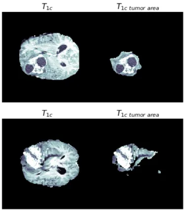
the first one (above) is a high grade subject while the second one (below) belongs to a low grade subject. Looking at this example it is easy to understand that the tumor grade isn’t just a measure of the overall dimensions: it’s a measure of how aggressive is this disease based on the appearance of the cells under a microscope and how malignant they look (cells and the organization of the tissue of an high grade do not look like normal cells). [30].

Figure 3.2. T1c tumor slice in HG (above) and LG (below) subjects.

Since we believe it is important to maintain the balance between HG and LG sub-jects during training and evaluation phases, we applied stratified sampling, following the approach of [31], in the splitting of the dataset in three different sets: training (80% of the original dataset was assigned to this set), validation (10%) and test (10%) with 219 patients assigned to the first set, 27 to the validation one and 28 to the test. Stratified sampling was used in order to show to the model, during training, the right amount of HG and LG without the risk of wrong generations once the model would have been used with the test set.

For example, let’s suppose that a generator of MRI scans is trained with a set containing only LG tumors. Then, when it comes the time to test this model with a new set, with completely unseen images of HG and LG tumors, our trained model would probably be able to generate good results when it receives a LG patient as input, while it would produce wrong synthesized images, especially in the tumor area,

(35)

3.3. Dataset

when it comes to generate the missing modality for a HG patient.

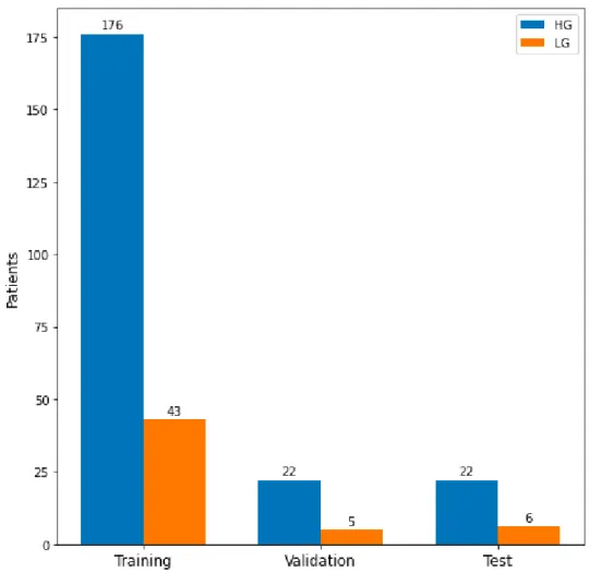
This explains why, in the splitting of the dataset, we chose to maintain a balance in the number of instances belonging to the two types of patient: stratified sam-pling allowed us to have HG and LG subjects represented with approximately equal proportions in all the three subsets, as it is shown in Figure 3.3.

Figure 3.3. Data distribution by set and tumor grade, after the split of BRATS2015 in Training (80%), Validation (10%) and Test (10%) using stratified sampling.

BRATS2015 contains basically images and few additional information about the patient: a unique identifier, not much useful, since data are anonymized (beside the fact we used it to find the correct ground truth folder of each volume), and whether the subject is a low grade or a high grade.

3.3.2 Images

The images are the most interesting part of the dataset: in total there are 1370 volumes and since, from each volume of the brain, it’s possible to extract 155 2D axial slices, with dimension 240x240 (an axial slice is one of the possible perspectives from

(36)

which is possible to represent the brain in two dimensions. The other two principal planes are the coronal and sagittal ones.), the number of available images is 212.350. The images are grayscale, so, instead of multiple color channels, there is just one channel that carries information and each value of a pixel represents only an amount of light.

Per each patient there are 5 volumes: 4 of these contain the different MRI sequences of the dataset (T1, T2, T1c, T2flair) while the last volume corresponds to the segmented

area of the tumor (in BRATS2015 this volume is called Ground Truth).

The modalities contained in the dataset are some of the most commonly acquired MRI sequences: we already discussed about T2-weighted (T2) and T2-fluid-attenuant

inversion recovery (T2flair). In addition to these two, we have T1-weighted (T1) and

T1-with-contrast-enhanced (T1c). These four scans provide both redundant and

complementary information about the imaged tissue and each one of this can give important and unique insights about the interested zone, in our case the brain.

T1 and T2f lair, for example, give meaningful information of the edema region of

tumor in case of glioblastoma. T1c on the other hand can become become very useful

when a contrast agent can be used with the patient, since it defines a clear demarcation of enhancing region around the tumor that can be used as an indicator to assess growth/shrinkage. T2 is used instead to detect hyperintensities that can lead to the

diagnosis of vascular dementia [1].

The 5th type of image given in this dataset is the one representing the tumor area (in BRATS2015 every subject has a brain tumor) that was used in this work to evaluate the results obtained by the trained models, as it happens in the segmentation task.

In segmentation though, these ground truths, made typically by one or more human experts, are used to quantify how good an automated segmentation is with respect to true tumor area.

The difference here is that we used the Ground Truth mainly as a mask applied to the synthesized images in order to discard the area of the brain not related to the tumor and then to compute the metrics and measure the quality of the generation only in that specific area, that is the most interesting and important one for the final diagnosis.

(37)

3.3. Dataset

(38)

Figure 3.5. T_{2flair masked}: tumor area obtained using the Ground Truth as mask over T_2flair.

3.4 Preprocessing

As in almost every deep learning pipeline, some preprocessing of the dataset was required: the details of the transformations applied to prepare the data in the proper manner are presented below.

3.4.1 Cropping

All the images in the dataset were first center cropped: the outer parts of each volume were removed while the central region was retained along each dimension.

This first preprocessing step reduced the dimensions of each volume from [240, 240, 155] to [180, 180, 128] but it’s important to notice that no useful information was removed but black voxels, so only the outer parts of the MRI with zero intensity value. This cropping brought also the advantage of having less heavy data in terms of size: removing useless information (as the black pixels around the brain) from a large dataset means, when it comes to read the data, less time to load the images in memory and obviously less memory needed to cache everything.

We observed that not all the 155 slices are equally relevant to us: some of the most external ones in the volume are totally black images while some contain just few pixels with intensity value different from zero.

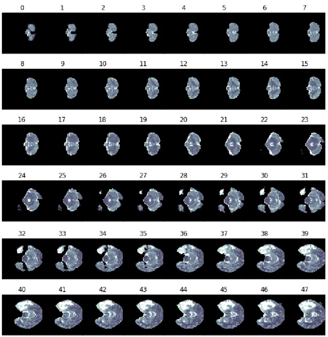
These images of course are meaningless for us since they contain neither enough information about the tumor nor significant brain structure that could be helpful to the GAN training: because of this we reduced the number of slices from 155 to 128. Figure 3.6 shows an example of the first 48, out of 128, T2 slices extracted from the

(39)

3.4. Preprocessing

Figure 3.6. An example of the first 48 T2 slices extracted from a volume, after cropping it to

(40)

3.4.2 Normalization

The motivation to normalize the images before feeding them into our models comes from the fact that in many machine algorithms it is required to have the same dynamic range, so the difference between the maximum pixel value and the minimum pixel value, per each image: in this way, by converting an input image to a range of pixel values that is more familiar and normal to the sense, it’s possible to avoid undesired effects.

In our case we used a type of rescaling known as min-max scaling or min-max normalization where the transformation, since we’re dealing with gray scale images, interested only one channel.

Min-max is the simplest normalization method and allows to bring the difference between the max value and the min value of an image to be in the range [a, b] using the following formula:

x0 = a + (x − min(x))(b − a)

max(x) − min(x) (3.1)

In our case we wanted to bring all the images to lie within the range of 0 to 1 by using the Formula 3.1 that with a = 0 and b = 1 becomes:

x0 = x − min(x)

max(x) − min(x) (3.2)

where, given a volume of a subject, x is the original intensity value and x’ is the new normalized voxel value. The min and max values were set to the values corresponding, respectively, to the 2nd and the 98th percentiles of the voxels intensities of the whole volume, to avoid the risk of using outliers in the normalization process: in fact we observed that in the dataset there are unusual high-intensity values due to pathologies and without this shrewdness these high values would have squashed the pixel range to always lie very close to zero.

Table 3.1 and 3.2 show how much important was to apply this processing step before actually starting to work with the data. Three volumes are used as example: the first two rows correspond to the same modality, T2, but different subjects while

the 2nd and the 3rd row show minimum value, maximum value, 2nd percentile and 9th percentile for the T2 and T2f lair of the same patient. The voxels values shown

can’t be really used without applying some scaling to the intensity channel neither to compare images from the same modality nor to evaluate volumes from the same patient.

(41)

3.5. Summary

Patient Modality Min value Max value 2nd Percentile 98th Percentile

0011_1 T2 0.0 1344.0 0.0 579.0

117_001 T2 0.0 2648.0 0.0 1013.0

117_001 T2f lair 0.0 720.0 0.0 389.0

Table 3.1. Values from different volumes before normalization

Patient Modality Min value Max value 2nd Percentile 98th Percentile

0011_1 T2 0.0 1.0 0.0 1.0

117_001 T2 0.0 1.0 0.0 1.0

117_001 T2f lair 0.0 1.0 0.0 1.0

Table 3.2. Values from different volumes after normalization

fixed percentile values: for example all the slices with 117_001 as patient id and

T2f lair as type of modality will be rescaled by using Formula 3.2 where 389.0 (the 98th

percentile) is the max value (instead of 720.0 that is an outlier value) and 0.0 (2nd percentile) is the min value. Results of the normalization are shown in Table 3.2.

This transformation step in the preprocessing phase was necessary because not all the images had the same dynamic range since BRATS2015 contains scans from multiple sources: the MRI volumes were obtained in different hospitals and with different acquisition settings (even the sequences of the same subject). By rescaling the whole dataset we were able to obtain more homogeneity among images, ranging now between 0 and 1.

3.5 Summary

In this chapter we presented some details about Magnetic Resonance Imaging, describ-ing the problem of missdescrib-ing modalities, and the reason why we focused our attention on brain tumor MRI scans.

We gave then an overview about the brain MRI dataset used in this work, BRATS2015, discussing how it is organized and which modalities it contains, showing also some figures to give an idea to the reader of the appearance of the different scans used to generate the missing modalities.

At the end of the chapter we described the preprocessing transformation useful to prepare the data before being fed into the models, whose architecture will be discussed in Chapter 4.

(42)

(43)

Chapter 4 System Design and Overview

The purpose of this chapter is to give a detailed description of how we optimized the input pipeline (Section 4.1) of our models and how we built the architecture of the networks used (Section 4.2) in this work. In Section 4.3 we present details from the training algorithm and which are the losses used in the update step, while Section 4.4 illustrates the evaluation metrics the we used in order to have a quantitative measure of how good were performing the trained networks.

4.1 Input Pipeline

After preprocessing the dataset with the transformations described in Section 3.4 (cropping and normalization), we proceeded to store the data as a TFRecord.

TFRecord, provided with the free and open-source software library of Tensorflow, is a format that allows large amount of data to be read in an efficient way [32] by serializing it and storing it as a sequence of binary records of varying sizes: GPUs, together with an efficient input pipeline (that starts from choosing the right data format), allow to achieve peak performance and to reduce computational times.

In order to build an highly performant input pipeline for the models we applied some important operations to our TFRecord data including a preprocessing step on the fly while loading data with the Data API :

• Caching the dataset in memory to save operations, such as file opening and data reading, from being executed during each epoch. It was crucial to apply this step before shuffling, batching and prefetching: data is read only once but is shuffled (next step) every time in a different way, with the next batch still being prepared in advance [19, p. 915].

(44)

• Shuffling the training set (with buffer size set to 128) since Gradient Descent works best when the instances are independent and identically distributed. • We then performed Mapping to decode efficiently the binary information and

store it into tensors. Inside this step, another processing transformation was applied to the data: a constant (zero - value) padding was added to images to reshape them as [256, 256, 128], i.e., a shape compatible with the input generator of the GANs implemented (see Section 4.2 for more details).

• Batching plays a major role in the training of deep learning models and because of this it was crucial to choose the right batch size based on the GPU available and on the neural networks that we were going to train.

Choosing the right batch size is important because it determines how many images are used to train the model before updating all the weights and biases. In our case we identify, after performing various experiments varying the batch size from 1 to 256, that 32 was the right number of images to use, at each iteration of the training algorithm, as input for all the models implemented.

Batch size Batches/epoch Train time/epoch (s)

1 1024 ≈ 500 4 256 ≈ 130 8 128 ≈ 75 16 16 ≈ 40 32 32 ≈ 30 64 16 ≈ 25 128 8 ≈ 23

256 4 GPU out of memory

Table 4.1. Train time/epoch of pix2pix using a reduced set of 1024 images.

Table 3.2 shows some of the experiments we performed to determine the proper batch size, evaluating the training time taken by pix2pix (Subsection 4.2.1) on GPU with a reduced dataset of 1024 images, varying the size of the batch and consequently the number of batches.

We noticed that a batch size equal to 256 couldn’t fit the GPU RAM provided by Google Colaboratory: the processors were running out of memory giving an error of resource exhausted. Furthermore, even though the training time was slower with respect to the times obtained with batch size of 64 and 128, we observed that 32 reached, qualitatively, more accurate results in the generated samples and [19, p. 681] explains the reason: in practice, large batch sizes often

(45)

4.2. Neural Networks Architecture

Figure 4.1. Example of single channel batch from the training set, with 32 T₁ slices cropped, normalized, shuffled and padded, with dimensions 256x256, ready to be fed to a single input model.

can lead to training instabilities and so the models may not generalize as well as a model trained with smaller batch size.

• Finally we applied a Prefetching step to have the preprocessing overlapping with the training execution: while the model is executing training step s, the input pipeline is saving time by reading data that will be used in the next training step s+1.

4.2 Neural Networks Architecture

In this work we developed two Generative Adversarial Networks: a multi-input version of pix2pix [6], that we called MI-pix2pix, and a modified version of the MM-GAN proposed by Sharma et al. in [1]. We also implemented pix2pix that was used mainly as a baseline to compare the performances reached by our multi-modal GANs, to see if they were producing better results, both in a qualitatively and quantitatively way.

In this section we discuss in detail the architectures behind these three GANs, showing also the differences between the model proposed by Sharma et al. and our modified version.

(46)

4.2.1 Pix2pix

Pix2pix is a single input - single output GAN, proposed by Isola et al. in [6] as a solution to the problem of image-to-image translation, extensively discussed in Subsection 2.2.5. This Generative Adversarial Network adopts a modified U-Net architecture [23] as generator and a PatchGAN [24] as discriminative model that tries to distinguish between the true samples coming from the dataset and the synthesized images of the generator.

Generator

In Subsection 2.2.5 we discussed about the strength of U-Net as generative network: skip connections between mirrored layers that represent a solution to the problem of losing information through the bottleneck layer. These connections are realized linking the i layer to the n-i layer (where n is the total number of layers) that receives as input a concatenation between the output of the i layer and the information processed by the n-(i+1) layer.

The generator architecture, with the U-shape from which U-Net takes its name, is illustrated in Figure 4.2. The input of the model is a tensor with size 32x256x256x1, where the first one indicates the batch size, so how many images are used per time for a single update. 64 Down1 128 Down2 256 Down3 512 Down4 512 Down5 512 Down6 512 Down7 512 Down8 512 Up1 512 Up2 512 Up3 512 Up4 256 Up5 128 Up6 64 Up7 ConvTranspose

Figure 4.2. Generator architecture from pix2pix [6].

In Section 4.1 we explained that it was necessary to add a padding to our images because otherwise they wouldn’t have been compatible to the input of the images: the problem with U-Net comes from the nature of its mirrored architecture and more in particular from its downsampling and upsampling layers that allow to have only input images with dimensions that are power of 2. We choose then to pad our 180x180

(47)

images in order to obtain a width and height of 256, instead of applying a resize/crop to 128: transformation that wouldn’t have preserved all the information in the images.

The input fed to the model goes first through the contracting path: a typical convolutional neural network (Subsection 2.2.1) composed by the repeated application of one the two main building blocks of the network, the downsample block, composed as follows:

• Convolution, that halves the dimensions of the input by convolving it through several filters with a fixed kernel size equal to 4 and stride of 2 for all the spatial dimensions.

• Batch Normalization in every block (with the exception of the first one). This operations zero-centers and normalizes each input, trying to overcome to the problem of the vanishing gradient [19, p. 728].

• Leaky ReLU, an activation function similar to ReLU but with a small slope for negative values useful to avoid that some neurons "die" during training (meaning that they stop outputting anything other than 0) [19, p. 720].

The repeated downsampling reduces the spatial information while increases the feature dimension, until the input arrives at the bottleneck where the output shape of the last downsampling block (Down7 ) is [1x1x512].

The building block that characterizes the expanding path of the network is instead the upsample block, composed by four layers:

• Transposed convolution that goes in the opposite direction of what is done by the Convolution, by enlarging the spatial information: image is first stretched with the insertion of empty rows and then a regular convolution is computed. A kernel size of 4 and stride of 2 was set in this layer.

• Batch Normalization

• Dropout, useful for its regularization effect against some possible overfitting, it was applied in the first three upsampling blocks.

• ReLU that has the advantage to not saturate for positive values (and it is fast to compute) [19, p. 720]

The last layer in the architecture of the generative part of [6] is another transposed convolution that prepares the output of the model with tanh (hyperbolic tangent) as

(48)

activation function, that returns values in a range between -1 and +1. The output of the network is a batch of images, 32 in our case, with dimension 256x256x1.

Discriminator

The PatchGAN [24] used to distinguish true images from fake images is similar to the well-known Convolutional Neural Network architecture (Section 2.2.1), with the difference that the discriminator of pix2pix doesn’t discriminate the whole image but small N xN patches of the input image: in this way the network can focus on capturing high frequencies details and assign to each patch a fake or true label.

This means that the output of the discriminator we used, in pix2pix and in the other GANs we experimented with, isn’t a 1x1 value but a 30x30 matrix, where each value contains the result of the discrimination over a 70x70 portion of the input image (the authors that developed [6] suggest to use a patch of this size to obtain the best

results from the GAN).

Because of this, the network used is called 70x70 PatchGAN and takes two inputs, as illustrated in Figure 4.3, each with shape [32, 256, 256, 1]: the first one is an input image while the second one is the target that can be an image coming from the dataset or a sample generated by the GAN.

64 Down1 128 Down2 256 Down3 512 Conv1 1 Conv2

Figure 4.3. Discriminator architecture from pix2pix [6].

The discriminator architecture, differently from the one of the generator, has only a contracting path and is composed by three downsample blocks that allow to reduce the spatial dimensions of the image while increasing the feature dimension. Each one of these blocks is characterized by a different number of filters (64 the first block, 128 the second one and 256 the last one) and they are defined with the same layers that

(49)

compose a downsample block in the generator (so batch normalization applied only in Down2 and Down3.

These blocks are then followed by several layers:

• Zero Padding, that doesn’t increment the number of trainable parameters, because it simply adds zeros at the top, left, right and bottom of an image. • Convolution with 512 filters, kernel size equal to 4 and stride of 1.

• Batch Normalization • Leaky ReLU

• Zero Padding

• Final convolution with 1 filter, again with kernels of 4x4 and stride set to 1. The description of the training algorithm used by pix2pix can be found in Subsection 4.3.2 while the implementation details are discussed in Subsection 4.3.3.

4.2.2 MI-pix2pix

MI-pix2pix is the second Generative Adversarial Network that we included in our experiments: it is a modified version of pix2pix [6] adapted to a multi-input scenario in order to compare and evaluate the differences between an unimodal approach and its variant that takes multiple modalities of available information as input.

Generator

The layers that compose the generator architecture (Figure 4.4) are the same as the ones that define the pix2pix model with the only difference in the input shape, that is set to [32, 256, 256, 3], while the output shape remains equal to [32, 256, 256, 1]. For example a MI-pix2pix that has to synthesize the missing T2 sequence of a subject will

use the information from the other three modalities available: T1, T1c, Tf lair that are

the inputs respectively of the first, second and third input channel.

Discriminator

Also for the Discriminator we maintained the same architecture (Figure 4.5) used in the unimodal version of pix2pix, but, since we are in a multi-modal setting, while the target has still a shape of [32, 256, 256, 1], the second input is a concatenation of the three modalities ([32, 256, 256, 3]) used to feed also the Generator.

(50)

64 Down1 128 Down2 256 Down3 512 Down4 512 Down5 512 Down6 512 Down7 512 Down8 512 Up1 512 Up2 512 Up3 512 Up4 256 Up5 128 Up6 64 Up7 ConvTranspose

Figure 4.4. Generator architecture from MI-pix2pix.

64 Down1 128 Down2 256 Down3 512 Conv1 1 Conv2

Figure 4.5. Discriminator architecture from MI-pix2pix.

MI-pix2pix was very useful to understand whether a multi-modal approach can exploit the information coming from different MRI sequences in a better way than what is done by pix2pix, since the two GANs share the same architecture and the same layers but receive a different number of images. The results of the comparison are presented in Chapter 5.

As for pix2pix, description of the training used can be found in Subsection 4.3.2 while the implementation details are discussed in Subsection 4.3.3.

(51)

4.2.3 MI-GAN

The third Generative Adversarial Network that we implemented is a multi-modal approach inspired by the work of Anmol Sharma and Ghassan Hamarhneh that in 2019 presented a multi-input multi-output GAN, called MM-GAN, that seems to be, to the best of their knowledge, the first method capable of synthesizing multiple missing sequences using a combination of various input sequences (many-to-many) [1].

Since the core of this work is on the generation of a single-output image, using different configurations and architecture of GANs, we focused our attention on a modified version multi-input single-output (many-to-one) of MM-GAN, called MI-GAN and implemented also by Sharma and Hamarhneh.

The focus of [1] was on the many-to-many approach though, and as a consequence many details about the MI-GAN model weren’t given: because of this, our model was inspired by the MM-GAN but at the same time it presents some variations that we applied, both to the architecture and to the loss used in the training algorithm (Subsection 4.3.2), in order to obtain a more stable training and satisfiable results in

the generated samples.

The layers that define the architecture of MI-GAN are almost the same proposed in [1] for the MM-GAN: the only variation applied was the replacement of every layer of Instance Normalization with a Batch Normalization, used also in pix2pix (Subsection 4.2.1) and in MI-pix2pix (Subsection 4.2.2), after observing through various experiments that normalizing the activations of each channel across the whole batch was more effective, in terms of quality in the generated samples, instead of computing the mean/standard deviation and normalizing across each channel in each training image.

Generator

The generator is a modified U-Net with concatenated skip connections and the typical U-shape architecture (Figure 4.6), characterized by two known building blocks: one that downsamples its input and one that, through a transposed convolution, performs an upsampling.

The downsample block is composed in a similar way to the one used in the previous model, with the addition of a dropout layer at the end of the block.

• Convolution with kernel size equal to 4 and stride of 2. • Batch Normalization in every block beside the first one. • Leaky ReLU

Brain magnetic resonance imaging generation using generative adversarial networks

Politecnico di Milano