Asymptotic time behaviour of nuclear systems : a Monte Carlo approach

(1)

POLITECNICO DI MILANO

Facolt`a di Ingegneria Industriale e dell’Informazione Corso di Laurea Specialistica in Ingegneria Nucleare

ASYMPTOTIC TIME BEHAVIOUR

OF NUCLEAR SYSTEMS:

A MONTE CARLO APPROACH

Relatore: PADOVANI Enrico Correlatore: ZOIA Andrea

Tesi di Laurea di: EPIFANO Enrica, matricola 787486

(2)

(3)

Ai miei nipotini, Francesco e Alessia

(4)

(5)

Abstract

In recent years, concerns about reactor safety have increased the need for computational methods that can provide accurate information about time-evolving scenarios, such as those occurring by design (transients, start-up, etc.) or by accident (rod ejection, for instance). In this respect, the atten-tion has been directed to the Monte Carlo methods, which are very accurate since introduce a minimal amount of approximations. Monte Carlo methods including the time dependence have been recently proposed: the Dynamic Monte Carlo methods, which allow assessing the complete time evolution of the neutron population. However, a non-negligible drawback is that these methods suffer from slow convergence and are very time-consuming. If one is interested in the asymptotic (long time) behaviour of the system, instead of the full time dynamics, a possible solution is to resort to the α-static Monte Carlo method, which is very accurate and less time-consuming than dynamic methods. This latter is the subject of this thesis.

We will show that the α-static Monte Carlo method allows determining the asymptotic time behaviour of the neutron population by transforming the time-dependent Boltzmann equation into an eigenvalue problem (the so called α eigenvalue). The mathematical theory at the basis of this method and the properties of the α-eigenvalue spectrum of the Boltzmann operator

(6)

will be explained; in particular, we will show that the asymptotic time be-haviour of the neutron population is dominated by the algebraically largest eigenvalue, named the fundamental eigenvalue. Then, we will present a Monte Carlo algorithm to solve the eigenvalue problem.

Finally, we will address the diffusion of neutrons in moderating materials and we will assess the asymptotic time behaviour of the system by using the α-static method. To this aim, during the work of this thesis, we have developed a Monte Carlo α-static code, based on the algorithm proposed, which provides the fundamental eigenvalue α0 and the associated eigenfunc-tion. We have also developed a dynamic Monte Carlo code, which can be used as reference to assess the time behaviour of the system. Finally, we have developed a deterministic solver, which provides a picture of the entire α-eigenvalue spectrum.

The key results of the simulations performed will be presented with a dou-ble aim: to validate the α static methods and to explore some interesting physical properties of moderators.

(7)

Sommario

Negli ultimi anni, la crescente attenzione verso la sicurezza dei reattori nucle-ari ha evidenziato la necessità di metodi computazionali che possano fornire informazioni accurate sulla dinamica degli scenari dipendenti dal tempo, sia quelli previsti by design (avvio del reattore, transitori di potenza, etc.) sia quelli incidentali, per esempio l’espulsione di una barra di controllo. In questo contesto, è naturale che l’attenzione si sia rivolta ai metodi Monte Carlo, nei quali le approssimazioni introdotte sono minime e, pertanto, sono molto accu-rati. Recentemente sono stati proposti dei metodi Monte Carlo che includono la dipendenza dal tempo: i metodi Monte Carlo dinamici, che permettono di stimare l’intera evoluzione temporale della popolazione neutronica. Tuttavia, questi metodi hanno un innegabile svantaggio: è necessario un considerevole tempo di calcolo per ottenere dati statisticamente validi. In alcune situazioni, può capitare che non sia necessario conoscere la dinamica completa del sis-tema considerato, ma che sia sufficiente il solo comportamento asintotico: in questo caso, una possibile soluzione consiste nel ricorrere al metodo Mon-tecarlo α-statico che, pur essendo molto accurato, richiede tempi di calcolo decisamente inferiori rispetto ai metodi dinamici. Questa tesi è incentrata proprio sul metodo α-statico.

Nel seguito, verr`a mostrato come il metodo α-statico, trasformando l’equazione

(8)

di Boltzmann dipendente dal tempo in un problema agli autovalori, consenta di trovare il comportamento asintotico nel tempo della popolazione neu-tronica. Nella tesi verranno descritte la teoria matematica alla base di tale metodo e le proprietà dello spetto degli autovalori α associati all’operatore di Boltzmann; in particolare, verrà dimostrato che il comportamento asintotico della popolazione neutronica è dominato dal più grande tra gli autovalori: l’ autovalore fondamentale α0. Successivamente, presenteremo un algoritmo Monte Carlo per risolvere il problema agli autovalori.

Infine, tratteremo la diffusione dei neutroni nei materiali moderatori e cercher-emo il comportamento asintotico del sistema usando il metodo α-statico. A tale scopo, durante questo lavoro di tesi, è stato sviluppato un codice Monte Carlo α-statico, basato sull’algoritmo proposto, capace di trovare l’autovalore fondamentale α0e l’autofunzione a questo associata. Abbiamo sviluppato an-che un codice Monte Carlo dinamico, il quale fornisce la completa evoluzione temporale del sistema; i dati forniti da questo secondo codice possono essere considerati i risultati di riferimento per valutare la correttezza delle infor-mazioni fornite dal codice α-statico. Infine, abbiamo sviluppato anche un solver deterministico, che fornisce l’intero spetto degli autovalori α. I risul-tati più importanti delle simulazioni effettuate verranno presentati con un duplice obiettivo: la validazione dei metodi α-statici e lo studio di alcune interessanti proprietà fisiche dei moderatori.

(9)

List of Figures

4.1 α-eigenvalue spectrum of the rod model for one-speed neutron transport . . . 41 4.2 α-eigenvalue spectrum for the neutron thermalization in an

infinite moderating medium . . . 44 4.3 α-eigenvalue spectrum for the neutron thermalization in a

bounded moderating medium . . . 48 4.4 Cross-sections modeling for crystalline moderators . . . 54 4.5 The α-eigenvalue spectrum for crystalline moderators . . . 55

5.1 Diffusion of one-speed neutrons in an infinite medium: the fun-damental eigenvalue α0 provided by the α-static code plotted as a function of the generations. . . 67 5.2 Diffusion of one-speed neutrons in a bounded medium: the

fundamental eigenvalue α0 provided by the α-static code plot-ted as a function of the generations. . . 68 5.3 Absorption and scattering cross-sections modeling . . . 69 5.4 α-eigenvalue spectrum (obtained by the deterministic solver)

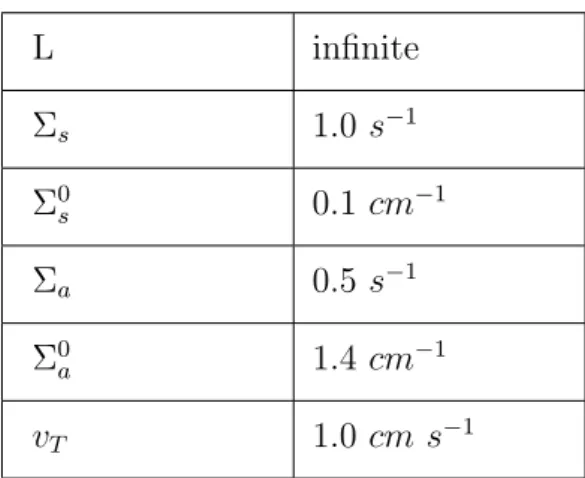
for the neutron thermalization in an infinite moderating medium with Σ0

a < Σ0 ∗a . . . 72

(14)

5.5 Neutron thermalization in an infinite medium with Σ0

a < Σ0 ∗a : the fundamental eigenvalue α0 provided by the α-static code plotted as a function of the generations. . . 73 5.6 The α-static results (blue) compared to the Dynamic Monte

Carlo results (green). . . 74 5.7 α-eigenvalue spectrum (obtained by the deterministic solver)

for the neutron thermalization in an infinite moderating medium with Σ0

a > Σ0 ∗a . . . 75 5.8 Neutron thermalization in an infinite medium with Σ0_a > Σ0 ∗_a :

the fundamental eigenvalue α0 provided by the α-static code plotted as a function of the generations. . . 76 5.9 The α-static results (blue) compared to the Dynamic Monte

Carlo results (green). . . 77 5.10 α-eigenvalue spectrum (obtained by the deterministic solver)

for the neutron thermalization in a one-dimensional bounded moderating medium . . . 79 5.11 α-eigenvalue spectrum (obtained by the deterministic solver)

for the neutron thermalization in a bounded moderating medium with L > L∗ . . . 83 5.12 Neutron thermalization in a bounded medium with L > L∗:

the fundamental eigenvalue α0 provided by the α-static code plotted as a function of the generations. . . 84 5.13 α-static results (blue) compared to Dynamic Monte Carlo

re-sults (green). . . 84 5.14 α-eigenvalue spectrum (obtained by the deterministic solver)

for the neutron thermalization in a bounded moderating medium with L < L∗. . . 85

(15)

5.15 Neutron thermalization in a bounded moderating medium with L < L∗: the fundamental eigenvalue α0 provided by the α-static code plotted as a function of the generations. . . 86 5.16 The α-static results (blue) compared to the Dynamic Monte

Carlo results (green). . . 87 5.17 Scattering cross section modeling for a medium with Bragg

scattering . . . 91 5.18 α-eigenvalue spectrum (obtained by the deterministic solver)

for the neutron thermalization in a moderating medium with Bragg scattering (L > L∗). . . 95 5.19 Neutron thermalization in a medium with Bragg scattering

(L > L∗): the fundamental eigenvalue α0 provided by the α-static code plotted as a function of the generations. . . 96 5.20 α-static results (blue) compared to Dynamic Monte Carlo

re-sults (green). . . 97 5.21 α-eigenvalue spectrum (obtained by the deterministic solver)

for the neutron thermalization in a moderating medium with Bragg scattering (L < L∗). It is possible to observe a single discrete eigenvalue in the gap between two continuum regions. 98 5.22 Neutron thermalization in a medium with Bragg scattering

(L < L∗): the fundamental eigenvalue α0 provided by the α-static code plotted as a function of the generations. . . 99 5.23 The α-static results (blue) compared to the Dynamic Monte

Carlo results (green). . . 100 5.24 Cross section modeling for slowing down and thermalization . 102

(16)

5.25 α-eigenvalue spectrum (obtained by the deterministic solver) for the neutron slowing down and thermalization in an infinite moderating medium with Σ0

a< Σ0 ∗a . . . 104 5.26 Neutron slowing down and thermalization in an infinite medium

with Σ0_a < Σ0 ∗_a : the fundamental eigenvalue α0 provided by the α-static code plotted as a function of the generations. . . . 104 5.27 The α-static results (blue) compared to the Dynamic Monte

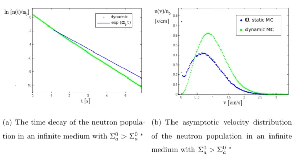
Carlo results (green). . . 105 5.28 The asymptotic velocity distribution in the pure

thermaliza-tion case (black) and in the slowing down + thermalizathermaliza-tion case (red). (Infinite medium with Σ0_a < Σ0 ∗_a ) . . . 106 5.29 The discrete eigenvalue α0 as a function of Σ0a for the neutron

slowing down and thermalization in an infinite medium. . . 107 5.30 α-eigenvalue spectrum (obtained by the deterministic solver)

for the neutron slowing down and thermalization in a bounded moderating medium with L > L∗. . . 109 5.31 Neutron slowing down and thermalization in a bounded medium

with L > L∗: the fundamental eigenvalue α0 provided by the α-static code plotted as a function of the generations. . . 109 5.32 The asymptotic velocity distribution in the pure

thermaliza-tion case (black) and in the slowing down + thermalizathermaliza-tion case (red). (Bounded medium with L > L∗) . . . 110 5.33 The discrete eigenvalue α0 as a function of L for the neutron

(17)

Chapter 1 Introduction

This thesis represents the final project for the Master of Science program in Nuclear Engineering of the Politecnico di Milano (Italy) and is the re-sult of a six months internship at the Service d’Etudes des Réacteurs et de Mathématiques Appliquées (SERMA) of CEA/Saclay.

The aim of the SERMA is the modelisation of nuclear systems, in particu-lar in the field of reactor physics and radiation shielding. My work has been carried out at the Laboratoire du Transport Stochastique et D´eterministe (LTSD), which conceives mathematical and numerical algorithms and devel-ops computer codes aimed at simulating radiation transport. In particular, the LTSD laboratory is in charge of developing the 3-dimensional continuous-energy Monte Carlo code TRIPOLI-4 R_.

Monte Carlo methods allow evaluating neutron and photon flux (i.e, solving the Boltzmann linear transport equation) by simulating the stochastic tra-jectories of neutrons and photons in phase space.

(18)

2

For historical reasons, also due to the limited computer power available at the time these methods were first introduced, Monte Carlo is mainly adopted to determine the stationary solution of the Boltzmann equation, where the time evolution can be safely neglected (the so called “static” calculations). In particular, in the context of radiation shielding Monte Carlo methods are typically used to solve for fixed-source problems, whereas in reactor physics they are typically used to determine the effective multiplication factor (keff) of the system and for this reason take the name of k-static methods. Generally speaking, Monte Carlo methods are very accurate, because they introduce a minimal amount of approximations, but they suffer from slow convergence and are thus more time-consuming than deterministic methods. In this re-spect, Monte Carlo simulation is typically adopted for performing reference calculations, against which the results of the faster (but approximated) de-terministic solvers are then validated.

In recent years, concerns about reactor safety have increased the need for computational methods that can provide accurate information about time-evolving scenarios, such as those occurring by design (transients, start-up, etc.) or by accident (rod ejection, for instance). In the context of Monte Carlo simulation, current research trends focus on dynamic methods, which follow the particles along their time evolution. Unfortunately, these methods demand an even larger computer time than static methods.

An intermediate bridge between static Monte Carlo and dynamic Monte Carlo is represented by the so-called α-static Monte Carlo. This method actually allows the prompt and delayed reactor period to be determined by transforming the time-dependent Boltzmann equation into a static

(19)

eigen-3

value problem (the so called α or time eigenvalue). In this respect, α-static methods are ideally suited so as to assess the asymptotic time behaviour of the system.

A Monte Carlo algorithm to find the α-eigenvalue has been recently de-veloped at the LTSD laboratory and implemented in the development version of the TRIPOLI-4 R

code.

The aim of this work is to verify and validate these new methods. The α-static Monte Carlo has been applied to the study of some simple physical systems: the outcomes of Monte Carlo simulations have been compared to reference results, coming either from exact analytical solutions (when avail-able), or from independent numerical codes. By virtue of this analysis, the strengths and the weaknesses of the α-static algorithm have been put in ev-idence, and an improved understanding of the method has been achieved.

This document is structured in five chapters:

1. In the first chapter, we shall familiarize with:

• time dependent problems concerning nuclear systems;

• the time dependent Boltzmann equation and its stationary form;

• the state-of-art numerical methods to solve the Boltzmann equa-tion.

2. In the second chapter, we shall focus on the α-static methods:

• the basic mathematical theory;

(20)

4

• the physical meaning of the fundamental discrete eigenvalue and some issues about its existence.

3. In the third chapter, we shall present some physical systems of interest and we will revisit the knowledge present in literature concerning their time behaviour, i.e. their α-eigenvalues spectrum.

4. In the fourth chapter, we shall show the results of our simulations. In particular, we shall compare the results of the α-static code to those coming from a dynamic Monte Carlo code and a deterministic solver.

5. Finally, in the last chapter, we shall explain our conclusions about the potentialities and the drawbacks of the α-static methods.

(21)

Chapter 2 Numerical methods for nuclear

systems

In this chapter, we shall introduce the Boltzmann equation governing the time-dependent neutron transport. We shall briefly discuss the numerical methods (deterministic and Monte Carlo) usually adopted to solve the sta-tionary form of this equation. Then, we will address the additional difficul-ties arising from explicitly considering the time dependence. Finally, we will evaluate the potentialities and the drawbacks of the recently proposed Monte Carlo methods for dealing with time-dependent systems: the dynamic Monte Carlo and the α static Monte Carlo.

2.1 The Boltzmann equation

Consider the statistical behaviour of a large population of neutrons in a bounded domain, under transient or steady state conditions. We define the particle density n(~r, v, ˆΩ, t) as the average number of neutrons present in

(22)

2.1. The Boltzmann equation 6

the infinitesimal volume of the six-dimensional phase space (~r ÷ ~r + d~r, v ÷ v + dv, ˆΩ ÷ ˆΩ + d ˆΩ) at time t. Starting from a given initial condition, the time evolution of the neutron density n(~r, v, ˆΩ, t) in a system is provided by the time-dependent linear Boltzmann equation, possibly coupled with the equations for the precursors concentrations c(~r, t) [3]. In neutron transport, it is reasonable to suppose the absence of particle-particle interactions (due to the weak neutron density as compared to that of the nuclei of the traversed medium [3]) and this implies that the equations are linear. The derivation of such equations is based on the principle of particle conservation in the phase space [3, 17, 20].

The linear Boltzmann equation for the neutron density reads ∂ ∂tn(~r, v, ˆΩ, t) + L n(~r, v, ˆΩ, t) = Fpn(~r, v, ˆΩ, t) + X i,j χi,j_d (~r, v) 4π λi,jci,j(~r, t) (2.1) where we have defined the linear transport operator

L f = v ˆΩ · ∇f + vΣtf − ∞ Z 0 Z 4π Σs(~r, v0 → v, ˆΩ0 → ˆΩ)v0f (~r, v0, ˆΩ0)d ˆΩ0dv0 (2.2)

and the prompt fission operator

Fpf = χp(~r, v) 4π ∞ Z 0 Z 4π νpΣf(~r, v0)v0f (~r, v0, ˆΩ0)d ˆΩ0dv0 (2.3)

Here notation is as follows: v is the neutron speed, ~r is the position vector and ˆΩ is the angular direction vector, Σt is the total cross-section, Σs is the differential scattering cross-section, χp is the normalized speed spectrum for prompt fission neutrons, νp is the average number of prompt fission neutrons, Σf is the fission cross-section, χi,jd is the normalized spectrum of delayed neu-trons emitted from precursor family j of isotope i, λi,j is the decay constant of precursor family j of isotope i and the double sum is extended over all

(23)

2.2. Stationary problems 7

fissile isotopes i in the system and over all precursor families j for each fissile isotope.

The Boltzmann equation for the neutron density is then coupled to the equa-tion for the evoluequa-tion of the precursor concentraequa-tion, which reads

∂ ∂tci,j(~r, t) = ∞ Z 0 Z 4π

ν_di,jΣi_fv0n(~r, v0, ˆΩ0, t) d ˆΩ0dv0− λi,jci,j(~r, t), (2.4)

where ν_di,j is the average number of delayed fission neutrons of precursor fam-ily j of isotope i.

The equations above are completed by assigning the proper initial and bound-ary conditions for n and ci,j.

For very short time scales t λ−1_ij , the impact of delayed neutrons can be safely neglected, so that we would have

∂

∂tn(~r, v, ˆΩ, t) + L n(~r, v, ˆΩ, t) = Fpn(~r, v, ˆΩ, t), (2.5)

but this is not the case for observation times t comparable to the decay lifetimes λ−1_i,j of the precursors [3]. Furthermore, we have assumed here that all physical parameters (such as cross-sections, energy spectra, and so on) are time-independent: this amounts to taking t shorter than the typical time scale of thermal-hydraulic and Doppler feedback [24, 1]. If N fissile isotopes are present, each associated to M precursors families, equations (2.1) and (2.4) form a system of 1 + N × M equations to be solved simultaneously. In the following we will address this issue.

2.2 Stationary problems

For customary problems emerging in reactor physics and radiation shielding, we are only interested in determining the steady-state of a system and we

(24)

can eliminate the time dependence from our equations. This can be achieved by resorting to two different approaches, depending on the physical situation we are dealing with.

The first approach emerges in radiation shielding calculations, where a fixed source Q is typically imposed. In this case, we simply integrate in time from zero to infinity in order to eliminate the time dependence.

By observing that we have ∂tn = ∂tc = 0, combing equations (2.1) and (2.4) yields

L n(~r, v, ˆΩ) = (Fp+ Fd)n(~r, v, ˆΩ) + Q(~r, v, ˆΩ) (2.6)

where n(~r, v, ˆΩ) is the stationary neutron density and

Fdf = X i,j χi,j_d (~r, v) 4π ∞ Z 0 Z 4π ν_dijΣf(~r, v0)v0f (~r, v0, ˆΩ0)d ˆΩ0dv0 (2.7)

Eq. (2.6) is again a balance equation: the total net disappearances (due to absorptions or leakage, minus scattering, which preserves the particle num-ber) must be balanced by the total productions (prompt and delayed fissions, if any) plus the contribution of the source.

The second approach emerges in reactor physics calculations, in which we are interested in finding the critical (i.e., stationary) core configuration. In this case, one tries to make the system time-independent by balancing the lack or the excess of neutrons through a “control coefficient”, named effective multiplication factor keff. Conceptually, keff can be defined as a scalar such that, if the number of neutrons generated by each prompt and delayed fission interaction is scaled by this number, the reactor is then artificially critical. Therefore, by setting the time-derivative to zero and introducing keff, Eq. (2.1)

(25)

becomes [3]

L n(~r, v, ˆΩ) = 1 kef f

(Fp+ Fd)n(~r, v, ˆΩ) (2.8)

where we have again collected the prompt and delayed fission terms. Remark that in this case we require Fp+ Fd > 0. Eq. (2.8) is formally an eigenvalue problem for the eigenvalue-eigenfunction pair {k, n} [8]. It can be shown that Eq. (2.8) admits an infinite number of discrete eigenvalues k under mild conditions about geometry, boundary conditions and cross sections [3, 17]; the corresponding eigenfunctions n = nk(~r, v, ˆΩ) are referred to as k-modes. The multiplication factor keff is the largest eigenvalue whose associated k-mode is everywhere non-negative (the so-called fundamental k-mode).

Since Eq. (2.8) has been made stationary by artificially introducing keff as a population control acting on the number of fission, the shape of the fun-damental k-mode is not expected represent any real neutron density except when the reactor is exactly critical, i.e., keff = 1. In other words, if we are dealing with a system that is far from critical and we solve Eq. (2.8) for this system, the obtained k-modes do not carry any physical meaning.

The main aim of Eq. (2.8) is to provide information concerning the value of keff for a given reactor configuration. If keff > 1 the reactor is supercritical, if keff < 1 the reactor is subcritical, and if keff = 1 the reactor is exactly critical. The system reactivity can be obtained as ρ = (k − 1)/k.

There are two methods for solving equations (2.6) and (2.8): the so-called deterministic approach, which basically consists in discretizing the solution in the space, energy and angle variables and solving the resulting linear system as a set of equations where the unknown is the vector containing the discretized solution; and the so-called stochastic approach, which consists in solving the equation by resorting to Monte Carlo methods. In the following, we will deal with the latter.

(26)

2.2.1 Monte Carlo transport theory

It can be shown [41] that the integro-differential equation (2.6) can be equiv-alently written in integral form:

ψ(~r, v, ˆΩ) = Z Γ ψ(~r0_{, v}0 , ˆΩ0_)K(~_r0 _{→ ~r, v}0 _{→ v, ˆ} Ω0 _{→ ˆ}_Ω)d~_r0_dv0 d ˆΩ0_{+ S(~}_{r, v, ˆ}_Ω), (2.9) where:

ψ = vΣt(~r, v)n(~r, v, ˆΩ) is the collision density, i.e., the average number of particles interacting with the matter at point (~r, v, ˆΩ) of the phase space;

K(~r0 _{→ ~r, v}0 _{→ v, ˆ}_Ω0 _{→ ˆ}_{Ω) = C(v}0 _{→ v, ˆ}_Ω0 _{→ ˆ}_{Ω, ~}_{r)T (~}_r0 _{→ ~r, v, ˆ}_{Ω) is the} trans-port kernel, which represents the particle density traveling from point (~r0_{, v}0_{, ˆ}_Ω0_{) of the phase space Γ and reaching point (~}_{r, v, ˆ}_Ω);

S(~r, v, ˆΩ) represents the first collision source and is equal to

S = R T (~r0 _{→ ~r, v, ˆ}_Ω)Q(~_r0_{, v, ˆ}_Ω)d~_r0_{, i.e., the average number of} parti-cles coming from the physical source Q(~r0_{, v, ˆ}_{Ω) and having their first} collision at point (~r, v, ˆΩ).

The transfer kernel T may be characterized by stating that, for a particle leaving a collision at point (~r0_{, v, ˆ}_{Ω), the expected number of next collisions} in the spatial volume Vr is:

Z Vr

T (~r0 _{→ ~r, v, ˆ}_Ω)d~_r. _(2.10)

If Vr represents an infinite medium, the integral must give 1, meaning that the event of a particle leaving position ~r0 _{and having a collision somewhere} in a infinite medium is a certain event.

(27)

The transfer kernel T reads

T (~r0 _{→ ~r, v, ˆ}_{Ω) = Σ}

t(~r, v) exp[−

Z Ω·(~ˆ r−~r0₎

0

Σt(~r0+ s ˆΩ, v)ds]. (2.11)

The collision kernel is defined so that, for a particle entering a collision at point (~r, v0, ˆΩ0_{), the expected number of particles leaving the collision in the} speed-direction volume VE is:

Z VE

C(v0 → v, ˆΩ0 _{→ ˆ}_{Ω, ~}_{r)dvd ˆ}_Ω. _(2.12)

The collision kernel reads

C(v0 → v, ˆΩ0 _{→ ˆ}_{Ω, ~}_{r) =} I X i pi(v0, ~r0)yi(v0)fi(v0 → v, ˆΩ0 → ˆΩ, ~r), (2.13) where:

pi(v0, ~r0) is the probability of undergoing reaction i out of a set of I possible reactions; it is represented by

pi =

Σi(v0, ~r0) Σt(v0, ~r0)

, (2.14)

i.e., the ratio between the reaction cross section Σi and the total cross section Σt;

yi(v0) is the multiplicity of secondary neutrons leaving reaction i;

fi(v0 → v, ˆΩ0 → ˆΩ, ~r) is the normalized distribution in the speed-direction space of secondary neutrons.

The sum of pi and the integral of the distribution function over the whole energy space are normalized to one. The multiplicity term yi(v0) depends on the reaction (it can be zero for absorption, one for scattering, or larger for other reactions).

(28)

Observe that we are assuming that the only transported particles are neu-trons. The coupling with other particles, such as for instance photons, will be neglected.

The Monte Carlo method for solving Eq. (2.9) (or equivalently Eq. (2.6)) consists in generating a large number of neutron random walks in the phase space so that their ensemble average converges to ψ (or n). Each random walk can be seen as the physical random trajectory of the transported particle, which travels along straight lines according to the transfer kernel T , separated by collisions with the nuclei, described by the collision kernel C. The random walks start from the source Q, have k collisions in the viable space and are eventually lost from boundaries or absorbed. Such random walks are defined by the set of coordinates in the phase space reached by the particles (for the sake of simplicity, from now on the coordinates in the phase space will be denoted by the point P = (~r, v, ˆΩ)).

The construction of the random walk is the basic step to be performed in order to simulate the transport of particles. Once the particle is created from the source Q, it travels through the phase space via the K(P, P0) kernel. Assuming full knowledge of the kernels at each point of the viable phase space, the random walks can be then generated by:

• sampling the traveled distance from the continuous density function of the transfer kernel T;

• sampling the reaction event from the discrete probability function pi;

• sampling the energy and the direction of the secondary particle after the collision from the continuous distribution function fi associated to the sampled reaction.

(29)

The topic of sampling techniques will be not approached in the following. Once an ensemble (i.e., a large collection) of random walks has been sam-pled, the purpose of a Monte Carlo simulation is in general to define the appropriate random variable ξ(α) associated to the random walk α whose expected value provides an estimate for the quantity:

E[ξ(α)] ≡ D n(~x) g(~x) E = Z Γ n(~x)g(~x)d~x, (2.15)

which represents the inner product of the particle density n(~x) times a general test function g(~x) on a defined volume of the phase space. The function g(~x) is precisely the score that is desired, and hn|gi represents the density-averaged score over the volume of interest. The quantity ξ(α), which must be properly chosen so to ensure the convergence E(ξ) = hn|gi, takes the name of Monte Carlo estimator [41]. The expected value of an ensemble of N random walks can be computed as:

E[ξ(α)] = P

nξ(αn)

N , (2.16)

where αn is the n − th random walk and ξ(αn) is the associated random variable. It can be shown [41] that convergence of the estimator as a func-tion of the number of simulated random walks goes with the square root of N .

The first kind of estimator is the so-called collision estimator, defined as:

ξcoll(α) = X m g(~xm) Σt(vm)vm , (2.17)

If we are interested in evaluating a score in a portion V of the phase space, the test function must be zero everywhere but in V ; in other words, the test function must be multiplied by the marker function χV(~x):

χV(~x) =    1 if ~x ∈ V 0 if ~x /∈ V

(30)

By progressively reducing the dimensions of such volume V , we can obtain the value of the score evaluated at a single point of the phase space. On the other hand, the smaller the volume, the smaller is the probability to obtain a sample of the event in that position. Special techniques exist to obtain an estimate of the pointwise distribution of a physical quantity in the phase space (the so-called point-flux estimation: here we will not address this issue). Observe that we have here considered density-averaged scores: more often, quantities of interests in reactor physics require averages over the neutron flux φ = nv. The corresponding flux estimator of collision type can be constructed as ξcoll(α) = X m g(~xm) Σt(vm) , (2.18)

which is such that E(ξ) = hφ|gi.

As an alternative to the collision estimator, the track estimator allows ob-taining a better estimation of density-averaged scores in small volumes. It is defined as [41]: ξtrack(α) = k X m=1 g(~xm)tm, (2.19)

where tm is the time spent by the m − th particle in the volume V of the phase space. For flux-averaged scores, we can then define

ξtrack(α) = k X m=1

g(~xm)dm, (2.20)

where dm is the track of the m-th particle in the volume V .

It can be shown [41] that, for any given g, we have ξtrack(α) ≡ ξcoll(α), which implies that the two estimators converge to each other when N → ∞, i.e., they are unbiased.

(31)

The variance associated to the estimators depends on the problem we want to solve. In general, the collision estimator (Eq. 2.17) works better in large volumes, whereas the track estimator (Eq. 2.19) is better suited for small volumes. We will make use of both in our simulations.

2.2.2 Monte Carlo power iteration

The Monte Carlo method for solving criticality problems, which are described by Eq. (2.8), is slightly different from the one just shown. In fact, in this case, we do not have a source distribution from which starting the particle random walks. However, Eq. (2.8) describes a linear eigenvalue problem that can be solved by power iteration method [26].

We can begin with a guess neutron distribution n0(~r, v, ˆΩ), called generation zero.

Then, we obtain the generation-one neutron density by applying a proper integral transport operator to the previous neutrons

n1(~r, v, ˆΩ) = K n0(~r, v, ˆΩ). (2.21)

and we find the first estimate of the k factor, which is given by the ratio

k1 = |n1| |n0|

. (2.22)

In order to avoid that neutron population goes to zero or diverges, we have to apply a population control, by dividing n1 for k1, so that we start the next generation with the same number of particles. We simulate the next gener-ation, starting the particle stories from the fission positions of the previous generation and we iterate this procedure for a large number M of neutron generations:

(32)

2.3. Time-dependent problems 16

In the limit of M → ∞, ki → kef f and the limit neutron density ni(~r, v, ˆΩ) is the eigenfunction associated to kef f [26].

2.3 Time-dependent problems

In chapter 2.2, we have seen how to solve the steady-state transport Boltz-mann equation by Monte Carlo methods. We now move to consider the full time-dependent Boltzmann equation.

Assessing the time behaviour of neutron transport is important in several situations of interest in nuclear engineering: reactor start-up, reactivity mea-surement, safety calculations, kinetics of accelerator-driven systems (ADS), only to name a few. In fact, the knowledge of the reactor kinetics is funda-mental both for normal scenarios (start-up, power transients) and accidental situations (rod ejection). Moreover, some reactor designs, such as the Ac-celerator Driven Subcritical system (ADS), intrinsically work at non-steady-state. The ADS has been investigated in the last decades as a promising tool to incinerate actinides and to transmute long-lived radioactive wastes. The nuclear fuel configuration is subcritical and an external neutron source (driven by an accelerator) is used to sustain the chain reaction. The time behaviour of such a system is subject to several transients and knowledge of the neutron dynamics is therefore needed [22].

In order to assess the reactor kinetics, we have to solve the time-dependent Boltzmann equation, which is a daunting task and demands special numer-ical methods so as to cope with the complexity of the involved system of equations.

(33)

2.3.1 Deterministic methods

Until now, the analysis of transient dynamics of a neutron population has been mainly carried out by resorting to deterministic methods. Here, for the sake of completeness we briefly recall some of the basic deterministic meth-ods [8, 22].

The direct method is a straightforward way to solve a time-dependent equation [8]. The time interval of interest is divided in small time sub-intervals [tj, tj+1], and for every sub-interval a stationary Boltzmann equa-tion is solved, by means of the usual numerical techniques (spatial discretiza-tion, multigroup energy approximations and so on). The direct method is complicated by the presence of very different time scales, which makes the Boltzmann equations a “stiff” system: indeed, an extremely fine time step is required to accurately describe the prompt-neutron behaviour (t ≈ µs) and a large number of time steps is required to represent the delayed-neutron behaviour (t ≈ s). Therefore, this method is seldom used.

The space-time factorization method is based on the idea of factorizing the neutron density into two parts: n(~r, ~v, t) = T (t)n0(~r, ~v, t) (for shortness, we have represented the angular dependence in the velocity vector), where the amplitude T depends only on time and the shape function n0varies slowly in time. Under this assumption, we can accurately obtain n0 even adopting large time-steps. Suppose now that the shape function is known. It can be shown [8] that, if we substitute the factorized density into Eq. (2.1) and Eq. (2.4) and we integrate over the space and energy domain weighting for

(34)

the adjoint flux, we obtain the point-reactor kinetics equations:

dT (t) dt = ρ(t) − β(t) Λ(t) T (t) + λc(t) (2.24) dc(t) dt = β(t) Λ(t)T (t) − λc(t) (2.25)

where ρ(t), β(t) and Λ(t) are the kinetics parameters defined in terms of the shape function n0 integrated in space and energy (therefore the only left dependence is on time). In particular, β(t) is the effective delayed-neutron fraction, Λ(t) is the neutron mean generation time and ρ(t) is the reactivity of the system, each depending on the time step. The actual implementation of the space-time factorization method is based on an iterative scheme. The shape function is first approximated by a known function in a large time step (shape step). With the approximated n0, the kinetics parameters β(t), ρ(t) and Λ(t) are calculated within the shape step. Equations (2.24) and (2.25) are then solved for the amplitude function T (t) with fine time steps (ampli-tude steps). Usually, the shape steps are several times larger than ampli(ampli-tude steps.

The modal expansion method is based on the hypothesis of total sep-aration between time dependence and space-energy dependence [8]. The approximated time-dependent solutions is written as

n(~r, ~v, t) =X n An(t)nαn(~r, ~v) (2.26) c(~r, t) =X n An(t)cαn(~r) (2.27) where nα

n and cαn are (precomputed) space-energy dependent expansion func-tions, the so-called α-modes and An(t) is the expansion coefficient for the nth_α-mode. _{The modes n}α

(35)

and (2.27) into equations (2.1) and (2.4) and solving the resulting equa-tions.

All such methods, even the direct method, introduce several approxi-mations, which are intrinsically due to the nature of deterministic solvers. Sometimes, it is desirable to have a higher-fidelity method for transient anal-ysis. In this respect, Dynamic Monte Carlo methods have been recently proposed to solve the time-dependent Boltzmann equation [22].

2.3.2 Dynamic Monte Carlo

The basic ideas behind Monte Carlo theory simulation have been recalled in chapter 2.2 as far as the solution of the stationary problems is concerned. As remarked, Monte Carlo methods solve the Boltzmann equation by simulat-ing particle histories, therefore introduce as few approximations as possible. The accuracy and the general applicability of these methods represent some of the reasons why many researchers and designers choose Monte Carlo sim-ulation, which is typically used as the reference for deterministic codes. A non-negligible drawback is that Monte Carlo in most practical cases turns out to be much slower than deterministic solvers. It is tempting to apply Monte Carlo methods also to transient calculations, which goes under the name of dynamic Monte Carlo method.

There are several new problems that need to be addressed in order to perform kinetic calculations with Monte Carlo codes [22]. First of all, the time factor, i.e., ∂n_∂t, is explicitly present, so that when sampling random walks we not only have to record the position in the phase space (~r, ~v) but also the time instants of birth, interaction and death of the particles. For

(36)

this reason, we have to split the time domain into bins and tally the scores of each event per bin. Moreover, a serious issue comes from the delayed neutron population. As we said, the time scale of delayed neutrons is much larger than that of prompt neutrons. In fact, while prompt neutrons are (almost) instantaneously emitted at fission events, the delayed neutrons come from the beta decay of precursors. Therefore, the probability density that a delayed neutron is emitted obeys the exponential decay law:

P (t) = λie−λit (2.28)

where λ is the specific decay constant of the ith _{precursor. In principle, when} a Monte Carlo simulation is performed, it is possible to sample νp prompt neutrons at the time of fission event tf ans sample νd delayed neutrons at time t = tf + td, where td is drawn from Eq. (2.28). This method mimics what actually happens in the physical system, but it would create too much variance, due to the very different time scales of the two populations [22]. Indeed, for a Monte Carlo calculation it is important to have enough statis-tics per tally bin. A possible remedy is therefore to force the precursors to generate a delayed neutron in each time bin; then, in order to obtain an unbiased score, we have to attribute to this neutron a modified statistical weight [22].

This algorithm is named forced precursors decay. With this method, all pre-cursors are stored, in order to have a decay in each time interval subsequent to the precursor appearance in the system. This implies that the total num-ber of precursors increases continuously. Therefore, population control is needed, not only for neutrons as customary, but also for precursors.

The precise details of the algorithm can be found in [22]. This prelim-inary discussion suggests that the explicit time dependence makes Monte

(37)

Carlo simulation much more complex than for static calculations. As a gen-eral rule, dynamic Monte Carlo methods demand an even larger simulation time than static simulations.

Despite all these drawbacks, dynamic Monte Carlo methods are quite appeal-ing for the reactor physics, and are goappeal-ing to be implemented in the devel-opment version of the Monte Carlo code TRIPOLI-4 R_{. This future version}

of the code will make possible to compute reactor power transients in regu-lar operation as well as in accidents, and eventually integrate the feedback coming from thermal-hydraulic codes.

2.3.3 Alpha static methods

In many practical situations, the knowledge of the full time dynamics of the system is not needed, and only the asymptotic (long time) behaviour is sought for. This is the case, for instance, of pulsed-neutron experiments or reactivity measures, where one is interested in determining the asymptotic relaxation of the system, following a given initial burst of neutrons at t = 0 [3, 17].

Asymptotic relaxation phenomena do not involve the solution of the full time-dependent Boltzmann equation, and can be dealt with by resorting to a different approach. The idea is similar to the modal expansion method, in which the neutron density is decomposed in a separated-variable form as

n(~r, ~v, t) =X n

An(t)nαn(~r, ~v). (2.29)

Indeed, in the analysis of asymptotic time relaxation, it is postulated that the neutron population obeys

n(~r, ~v, t) =X α

(38)

so that for long times we have

n(~r, ~_{v, t) ≈ n}α0(~r, ~v)e

α0t_, _(2.31)

where α0 is the algebraically largest value among all α of the expansion. In other words, we are assuming that the neutron population at long times will grow or decay in an exponential fashion, with asymptotic period given by α0. As for the space and velocity behaviour, Eq. (2.31) implies that at long times the functional shape of n will not change anymore, and will be given by n ≈ nα0(~r, ~v). As for the precursor population, it is similarly demanded

that

c(~r, t) =X α

cα(~r)eαt. (2.32)

If we are interested in knowing the complete time behaviour of n(~r, v, ˆΩ, t) and c(~r, t), we should replace the full expansions (2.30) and (2.32) into the Boltzmann equation and explicitly solve the resulting equations. However, due to the postulated exponential nature of the neutron and precursor pop-ulations, after a transient, only the term with the algebraically largest coef-ficient α0 will survive. Therefore, in order to assess the asymptotic neutron and precursor behaviour, we are led to consider only the dominant frequency α0.

By replacing n = nαeαt and c = cαeαt into Eq. (2.1) and Eq. (2.4) respec-tively, we get a set of coupled equations

αnα(~r, v, ˆΩ) + L nα(~r, v, ˆΩ) = + FP nα(~r, v0, ˆΩ0) + X i,j χi,j_d (~r, v) 4π λi,jc i,j α (~r) (2.33) and αci,j_α (~r) = ∞ Z 0 Z 4π

(39)

which are formally a system of eigenvalue equations, whose dominant eigen-value is precisely α0 [3]. Equations (2.33) and (2.34) do not depend on time anymore and therefore look like static equations (in a sense that will be made clear in the following chapter). Due to the presence of the α term, eqs. (2.33) and (2.34) take the name of α-static equations: the next chapter will be de-voted to the specific Monte Carlo methods conceived to assess the asymptotic time behaviour of nuclear systems by solving the α-static equations.

We conclude by observing that approximating the full expansion (2.30) with the fundamental mode nα0e

α0t _{is formally equivalent to adopting the}

space-time factorization with a time-independent shape function: n(~r, ~v, t) = T (t)n0(~r, ~v). In this case, the kinetics parameters previously introduced, namely ρ, Λ and β, are all constant. Therefore, equations (2.24) and (2.25) simply become the point kinetic equations:

dT (t) dt = ρ − β Λ T (t) + λc(t) (2.35) dc(t) dt = β ΛT (t) − λc(t). (2.36)

(40)

(41)

Chapter 3 The α static methods

In the previous chapter, we have introduced the α-static method. In this chapter we shall make clear the mathematical basis of this method and then we shall introduce the algorithm developed in TRIPOLI-4 R_.

3.1 The mathematical theory

The full time behaviour of the neutron density in a system is provided by the time-dependent Boltzmann equation

∂ ∂tn(~r, v, ˆΩ, t) + L n(~r, v, ˆΩ, t) = Fpn(~r, v, ˆΩ, t) + X i,j χi,j_d (~r, v) 4π λi,jci,j(~r, t) (3.1) coupled with the precursor equation (2.4)

∂ ∂tci,j(~r, t) = ∞ Z 0 Z 4π

ν_di,jΣi_fv0n(~r, v0, ˆΩ0, t) d ˆΩ0dv0− λi,jci,j(~r, t). (3.2)

(42)

3.1. The mathematical theory 26

When the long-time (asymptotic) behaviour is sufficient so as to characterize the system evolution [3, 17], an exponential relaxation of the kind

n(~r, v, ˆΩ, t) = nα(~r, v, ˆΩ)eαt (3.3)

and

ci,j(~r, t) = ci,jα (~r)e

αt _(3.4)

is postulated for both the neutron flux and the precursors concentrations, where the parameter α (carrying the units of the inverse of a time) plays the role of the inverse of the asymptotic relaxation time scale [3, 17]. Equa-tions (3.3) and (3.4) formally stem from imposing the separation of variables in Eqs. (3.1) and (3.2), and can be more rigorously justified by resorting to Laplace transform analysis or equivalently to spectral analysis [17]. Yet, proving the feasibility of such exponential relaxation is highly non-trivial in general, and precise (although not very restrictive) conditions are required on the geometry of the domain and on the material cross-sections [3, 17, 28]. We shall discuss this issue later.

Replacing Eqs. (3.3) and (3.4) into Eqs. (3.1) and (3.2), respectively, yields the so-called α-static equations

αnα(~r, v, ˆΩ) + L nα(~r, v, ˆΩ) = + FPnα(~r, v0, ˆΩ0) + X i,j χi,j_d (~r, v) 4π λi,jc i,j α (~r), (3.5) αci,j_α (~r) = ∞ Z 0 Z 4π

ν_di,jΣi_f(~r, v0)vnα(~r, v0, ˆΩ0) d ˆΩ0dE0− λi,jci,jα (~r), (3.6)

which form a stationary, coupled system, formally representing an eigenvalue problem. Finally, solving with respect to nα results into the (nonlinear) eigenvalue problem [3, 43, 9, 19] αnα(~r, v, ˆΩ) + L nα(~r, v, ˆΩ) = Fpnα(~r, v, ˆΩ) + X i,j λi,j λi,j+ α F_di,jnα(~r, v, ˆΩ), (3.7)

(43)

where α is the eigenvalue and nα the associated eigenmode, and we have defined F_di,jf = χ i,j d (~r, v) 4π ∞ Z 0 Z 4π ν_di,jΣi_f(~r, v0)f (~r, v0, ˆΩ0) d ˆΩ0dv0. (3.8)

In principle, Eq. (3.7) has 1 + N × M sets of eigenvalues (one prompt and N × M delayed eigenvalues) associated to each eigenmode nα [3, 9, 19]. In order to determine the asymptotic time behaviour of the system, Eq. (3.7) must be solved for the algebraically largest eigenvalue α, so that the corre-sponding fundamental mode nα(~r, E, ˆΩ) will provide the asymptotic space, angle and energy shape of the neutron flux at long times. We shall treat the problems of the prompt and delayed behaviour separately.

3.1.1 The prompt behaviour

When delayed contributions can be neglected (i.e., F_di,jnα = 0), α is called the prompt time eigenvalue: the mathematical properties of the resulting (linear) eigenvalue equation

αnα(~r, v, ˆΩ) + L nα(~r, v, ˆΩ) = Fpnα(~r, v, ˆΩ) (3.9)

and the numerical schemes for assessing the dominant eigenvalue have been the subject of considerable research efforts (see for instance the comprehen-sive works [3, 17, 28, 2] about theoretical aspects and [21, 6, 15, 39, 45, 34, 48] concerning numerical methods).

(44)

Knowledge of the spectrum σ(A) of the Boltzmann operator

A f = (− L + Fp)f = −v ˆΩ · ∇f − vΣtf + ∞ Z 0 Z 4π Σs(~r, v0 → v, ˆΩ0 → ˆΩ)v0f (~r, v0, ˆΩ0)d ˆΩ0dv0+ χp(~r, v) 4π ∞ Z 0 Z 4π νpΣf(~r, v0)v0f (~r, v0, ˆΩ0)d ˆΩ0dv0 (3.10)

is fundamental so as to determine the properties of Eq. (3.9) and in partic-ular of its dominant eigenvalue and eigenmode.

3.1.1.1 Finite spatial domain

An exhaustive analysis of the spectrum σ(A) of the Boltzmann operator A has been provided by Larsen and Zweifel in [28] for a broad class of collision kernels and geometries. Here, we recall the main results [28] for the eigenvalue problem

A nα = αnα.

We define A in an L1(D × V ) space, where D is the bounded spatial domain and V is the velocity domain, i.e., v0 < v < v1, where v0 < v1 < c, c being the speed of light. First, we consider the streaming and removal operator T , defined as

T = −[~v · ∇r+ vΣT(~r, v)]. (3.11)

Let us denote v0 the minimum allowed neutron speed. It can be then shown that [28]:

• If v0 > 0, then the spectrum σ(T ) consists solely of the point at infinity: σ(T ) = {∞}.

(45)

• If v0 = 0, then the spectrum σ(T ) consists of the complex half plane: σ(T ) = {α | Re{α} ≤ α∗}, where α∗ _{= − lim}

v→0vΣT(v).

The spectrum σ(T ) of the operator T may then contain a continuum por-tion. The limiting value α∗ takes the name of Corngold limit and physically represents the minimum collision frequency. We consider now a one-speed transport operator A0, defined as

A0 = T + K0, (3.12)

where K0 is a collision operator that does not change the neutron speed. This operator describes a purely elastic or Bragg scattering and has the form

K0f = Z

v0

k0(~r, v0, ˆΩ0 → ˆΩ)δ(v0 → v)f (v0)dv0 (3.13)

Therefore, the operator A0 does not change the neutron speed and depends only parametrically upon v. It can be shown [28] that the one-speed operator A0 has a spectrum σ(A0) entirely formed by isolated eigenvalues, for fixed v. The eigenvalues depend parametrically upon the neutron speed. In general, as v varies between v0 and v1, some of the eigenvalues will remain stationary and some will shift and trace out curves. Thus, the spectrum σ(A0) will consist of isolated points and curved lines. As in the previous case, if we allow v0 = 0 there will be also a continuum half-plane in the α-spectrum.

Finally, we consider the general case where the transport operator A is

A = T + K, (3.14)

where K is the scattering operator, physically corresponding to fission, slow-ing down, thermal scatterslow-ing and Bragg scatterslow-ing.

(46)

spectrum σ(T + K0) only by the addition of a point spectrum.

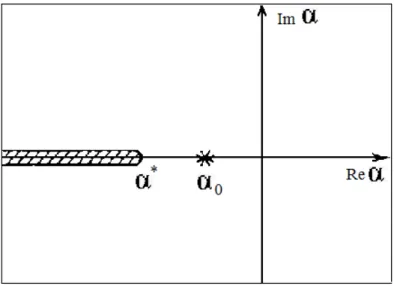
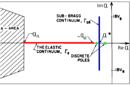
Summarizing, the collision terms of the Boltzmann operator contribute to the α-spectrum σ(A) with discrete eigenvalues and (Bragg scattering) curves. The streaming operator may induce (under the assumption of v0 = 0) the presence of a continuum half-plane in the spectrum. If this is the case, a question of utmost importance concerns the existence of a simple dominant eigenvalue, i.e., a simple eigenvalue α0 whose real part is larger than any other α in the spectrum, and whose associated eigenfunction nα is non-negative. In fact, if a continuum portion is present in the spectrum σ(A), the neutron density expansion (2.30) must be written in the more general form

n(~r, ~v, t) =X α nα(~r, ~v)eαt+ Z α∗ −∞ G(α)nα(~r, ~v)eαtdα, (3.15)

where G(α) are weight functions expressing the amplitude density of each continuum eigenfunction. If the fundamental eigenvalue exists (i.e., if the discrete sum in Eq. (3.15) is not empty), the asymptotic behaviour will be dominated by the exponential term with α = α0. If α0 ≤ α∗, the discrete spec-trum disappears into the continuum and the sum in Eq. (3.15) is empty. In this case, the asymptotic behaviour of the neutron density will be dominated by the continuum and it will not be possible to extract a single dominant exponential decay [17]. It can be shown that α0 disappears into the contin-uum if the radius of the domain D is smaller than a critical value, which is typically of the order of a mean free path [32, 44].

3.1.1.2 Infinite spatial domain

We now discuss the behaviour of the spectrum σ(A) for infinite spatial do-mains. An analysis of this case has been provided by Duderstadt [17] and

(47)

Corngold [13]. We have again an eigenvalue problem of the type:

A nα = αnα. (3.16)

Maintaining the same notation, the operator A is given by A = T + K. In this case, the streaming and removal operator T is simply

T = −vΣT(v) (3.17)

and K is the scattering kernel. Note that, under the assumption of infinite and homogeneous medium, the angle and position dependencies have been eliminated by integrating over these variables.

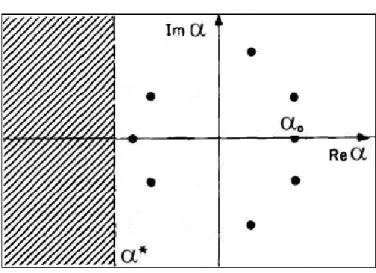
The spectral analysis of Duderstadt [17], carried out under the hypothesis of allowing v0 = 0, shows that the spectrum σ(A) of the Boltzmann operator A for an infinite medium is composed by:

• a continuum unidimensional set σc(A) = {α : α = −vΣt(v), v ∈ [0, ∞)}

• a real discrete set of eigenvalues α ≥ α∗_{, where α}∗ _{= − lim}

v→0vΣT(v). Corngold has shown [13] that the properties of the discrete set depend on the scattering kernel considered, i.e., on the diffusion properties of the medium. For example, for incoherent solids, the discrete eigenvalues are finite in num-ber. Ordinarily, only few discrete α exist, or sometimes only the fundamental α0 exists. It is also possible, by introducing an absorption rate Σa(v)v which increases sufficiently strongly with v, to have an empty discrete set. On the contrary, for gases, we find an infinite set of discrete eigenvalues, with α∗ ap-pearing as a limit point of this set. In this case, the possibility of an empty point spectrum, by introducing an absorption rate strongly increasing with v, is not realistic.

(48)

3.1.2 The α-problem with delayed neutrons

The full Eq. (3.7)

αnα(~r, v, ˆΩ) + L nα(~r, v, ˆΩ) = Fpnα(~r, v, ˆΩ) + X i,j λi,j λi,j+ α F_di,jnα(~r, v, ˆΩ)

including delayed contributions (in which case α is called the delayed time eigenvalue, and physically represents the inverse of the reactor period) has received comparatively less attention (see for instance [3, 9, 19, 23] for a survey) but has recently attracted renewed attention [22, 7, 40, 31] in view of the practical applications in reactor kinetics. Indeed, integrating Eq. (3.7) over all phase space variables leads to the reactor inhour equation [3]

ρ0 = αΛ0+ X i,j α λi,j+ α β₀i,j (3.18)

where ρ0 = (k0 − 1)/k0 is the reactivity, with

k0 = h1, Fpφα+ P i,jF i,j d φαi h1, L φαi , (3.19)

Λ0 is the mean generation time

Λ0 =

h1,1 vφαi

h1, Fpφα+P_i,jF_di,jφαi

, (3.20)

and β₀i,j are the flux-averaged delayed fractions

β₀i,j = h1, F i,j d φαi h1, Fpφα+ P i,jF i,j d φαi , (3.21) with P i,jβ i,j

0 = β0. In the equations (3.19), (3.20), and (3.21), the impor-tance function has been chosen equal to 1. From Eq. (3.18) it is apparent that α plays the role of the reactor period in the inhour equation.

(49)

3.2. The proposed algorithm 33

3.2 The proposed algorithm

We present now a Monte Carlo method to find the dominant eigenvalue α0. We begin with the algorithm for prompt eigenvalue (the equation without delayed contributions) and then extend it so as to cover the full Eq (3.7). The fundamental eigenvalue α0 can be estimated via Monte Carlo methods by adapting the power iteration algorithm for k static criticality calculations (described in Chapter 2). The method is then called α-k power iteration al-gorithm and its specific details depend on the sign of the dominant eigenvalue α [21, 6, 15, 48]. In the following, we sketch the structure of the algorithm by considering supercritical (α > 0) and subcritical (α < 0) configurations separately.

3.2.1 Positive dominant eigenvalue, α > 0

When F_di,jnα = 0 and α > 0, Eq. (3.7) can be identically rewritten as [21, 6]

Lαnα(~r, v, ˆΩ) = 1

k Fpnα(~r, v, ˆΩ), (3.22) where Lα = L +Σα is a modified transport operator, Σα = α and α is to be determined such that the fictitious parameter k = 1 in Eq. (3.22) . By re-marking that the positive term Σα can be interpreted as an additional sterile capture cross-section added to the total cross section, the usual α-k power iteration algorithm is applied as follows: we start from a tentative distri-bution n0

α (zero-th iteration) for the neutrons and provide a guess value for α0. Then, we search for the corresponding k eigenvalue by standard power iteration, which will depend on the current value of α. On the basis of k, we will then adjust the value of α for the next generation (for instance, one can take αj+1 _{= kα}j_{). This procedure is iterated until k converges to k = 1: the}

(50)

3.2. The proposed algorithm 34

corresponding value of α will provide the fundamental prompt eigenvalue, and the associated nα the fundamental eigenmode.

The delayed contributions can be included [50] by rewriting

Lαnα(~r, v, ˆΩ) = 1 k " Fpnα(~r, v, ˆΩ) + X i,j λi,j λi,j + α F_di,jnα(~r, v, ˆΩ) # , (3.23)

where the factor

γi,j = λi,j/(λi,j+ α) > 0 (3.24)

in front of the F_di,j terms acts as a population control tool to be applied to each delayed neutron coming from delayed fission. This means that the weight of delayed neutrons is first multiplied by a factor γi,j and then divided by a factor k before being assigned to the next generation.

3.2.2 Negative dominant eigenvalue, α < 0

When F_di,jnα = 0 and α < 0, the standard α-k power iteration algorithm applied to Eq. (3.7) is known to be numerically unstable and usually leads to abnormal code termination [21]. In reference [48] an improved algorithm for negative α has been provided and shown to be numerically stable. The key ingredient consists in rewriting Eq. (3.7) as follows

Lα,ηnα(~r, v, ˆΩ) = 1 k h Fpnα(~r, v, ˆΩ) + Fα,ηnα(~r, v, ˆΩ) i , (3.25)

where Lα,η = L +Σα,η, Σα,η = −ηα (η being an arbitrary positive constant) and we have formally defined the creation operator

Fα,ηf = ∞ Z 0 Z 4π νηδ(v − v0)δ( ˆΩ − ˆΩ0)Σα,ηf (~r, v0, ˆΩ0)v0d ˆΩ0dv0 (3.26)

(51)

3.3. Verification tests 35

with νη = (η + 1)/η > 0.

The term Σα,η acts here as an additional creation cross-section, whose asso-ciated creation operator Fα,η appears at the right hand side of the equation (with a delta-spectrum in energy and angle). Then, Eq. (3.25) can be solved by applying the power iteration similarly as done above. Observe in particu-lar that Eq. (3.25) holds also for moderating materials, where Fpφα vanishes: in this case, neutrons are promoted to the next generation of the power iter-ation algorithm only via the creiter-ation operator Fα,η [48].

Including delayed contributions [50] leads to

Lα,ηnα = 1 k " Fpnα+ Fα,ηnα+ X i,j γi,jFdi,jnα # , (3.27)

where again the factor γi,j = λi,j/(λi,j + α) in front of the Fdi,j terms acts as a population control tool. Observe however that now γi,j introduces singu-larities in Eq. (3.27) at the values α = −λi,j, α being negative. If we restrict our search to the dominant α eigenvalue, this implies that α must be found in the interval −λα < α < 0, where λα = mini,jλi,j is the smallest decay constant over all fissile isotopes and over all precursors families. Bearing this consideration in mind, the treatment of delayed neutrons proceeds as above, i.e., the weight of delayed neutrons is first multiplied by a factor γi,j and then divided by a factor k before being assigned to the next generation.

3.3 Verification tests

The Monte Carlo method discussed above has just been recently implemented in the development version of the Monte Carlo code TRIPOLI-4 R_.

(52)

3.3. Verification tests 36

The aim of this work is to verify and validate the α-k power iteration algo-rithm in some specific situations. We have seen in paragraph 3.1 that, under the hypothesis of minimum neutron speed v0 = 0, the α spectrum contains a continuum half-plane. We have also seen that all discrete eigenvalue might disappear into the continuum, so that a fundamental α eigenvalue does not exist anymore, and the asymptotic decay is not exponential.

Then, what is the behaviour of the α-static code in this particular situation? Does it converge to any value and, if this is the case, can we associate a physical meaning to this value? What is the shape of the associated eigen-function, if any? We shall try to answer these questions.

Actually, a word of caution is necessary here. As we said, the presence of a continuum portion in the spectrum σ(A) intrinsically depends on the min-imum neutron velocity v0 being allowed to vanish, i.e., v0 = 0. In industrial Monte Carlo codes, such as TRIPOLI-4 R_{, this can not happen in}

prac-tice: the tabulated continuous-energy cross sections typically assume that E0 ∼ 10−5eV , whence v0 ∼ 44 m/s. Then, v0 being small but non-vanishing, a dominant eigenvalue surely exists and the questions above can not be sim-ply answered within the code. For this reason, we have developed a specific (and simplified) α-static Monte Carlo code for testing the α − k algorithm. This allows also simple hypotheses and transport models to be checked sep-arately, without being hindered by the full complexity of the TRIPOLI-4 R

code. The results of our α-static code have been verified against exact or numerical solutions, when available. Also, an analog dynamic Monte Carlo code has been developed, with the aim of performing dynamic simulations by following neutrons in time: this latter code has been used so as to validate the α-static algorithm. This work will be detailed in the following.

(53)

Chapter 4 Physical models for neutron

transport in moderating

materials

Our aim being the verification and validation of the α-static method, we look for reasonably simple nuclear systems where analytical or numerical solutions are easily available and can therefore be used as a reference. Starting from the full time-dependent Boltzmann equation, we will introduce a series of simplifications that will allow reaching our goal, yet retaining the key physical features of the systems at hand.

Under these assumptions, we will recall here the key results concerning the fundamental time eigenvalue and the associated fundamental eigenmode for such systems. Only moderating configurations will be examined. The results obtained in this chapter will be used in Chapter 5 to validate our α-static code.

(54)

4.1. One-speed neutron diffusion 38

namely, the diffusion of thermal neutrons through a medium when multipli-cation (fission) is neglected.

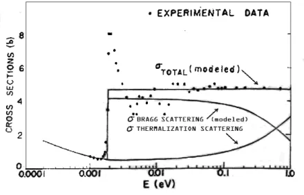
Such situation occurs in the analysis of asymptotic relaxation phenomena in neutron thermalization [44, 17] . For instance, one may be interested in injecting a burst of neutrons in a sample,and measuring the subsequent de-cay of the neutron population as a function of time. Such pulsed-neutron experiments provide information about the neutron transport parameters (such as the diffusion coefficient) and have been extensively performed in the sixties so as to characterize various moderating materials, such as water or graphite [13].

We begin our analysis by considering the diffusion of one-speed neutrons in an infinite medium. Then, we take into account finite-size effects by in-troducing the simplest possible leakage model, the so-called rod model. Next we address the thermalization of continuous-energy neutrons in two differ-ent kinds of moderators: the hydrogen-based moderators and the crystalline moderators. Finally, we treat the case of fast neutrons transport.

4.1 One-speed neutron diffusion

4.1.1 Infinite medium

In the case of one-speed transport in an infinite homogeneous medium, cross sections are constant and Eq. 2.1 simplifies to:

∂

∂tn(t) + Σtvn(t) = Σsvn(t), (4.1)

where n(t) = R 4π

n( ˆΩ, t)d ˆΩ is the neutron density integrated over directions. Note also that, in this simple case, the cross sections become constants. The one-speed transport model is quite trivial, yet provides a rough idea of the

(55)

4.1. One-speed neutron diffusion 39

asymptotic time behaviour of a moderating system.

Recalling equation 4.1, and observing that Σt = Σs+ Σa, we simply have

n(t) = n0e−Σavt, (4.2)

where n0 = n(t = 0) is the initial condition for the neutron density. Neutrons disappear from the system with a decay constant equal to the absorption rate: this means that α0 = −Σav, which provides a first elementary check for α-static methods.

4.1.2 The rod model

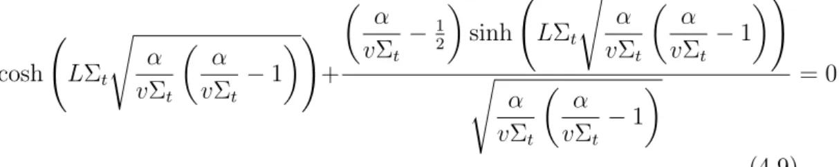
In order to go a step further in our analysis, we must include finite-size effects due to spatial boundaries. To simplify the matter, we will consider the so-called rod model. Neutrons move on a 1-dimensional interval [0,L], where only two directions are allowed (forward and backward). Moreover, we assume that scattering is isotropic. The system has been extensively used in reactor physics [17, 30, 46, 48, 49] because it is rather easily amenable to analytical solutions and yet retains the key mechanisms of leakages from the boundaries.

The Boltzmann equation for rod model degenerates in two coupled linear differential equations for the two components of the angular density, namely,

∂ ∂tn + (x, t) + Σtvn+(x, t) + v ∂ ∂xn + (x, t) = 1 2Σsv[n + (x, t) + n−(x, t)] (4.3) ∂ ∂tn − (x, t) + Σtvn−(x, t) − v ∂ ∂xn − (x, t) = 1 2Σsv[n + (x, t) + n−(x, t)] (4.4)

where n+(x, t) = n(x, ˆΩ = +, t), n−(x, t) = n(x, ˆΩ = −, t) and x is the spatial coordinate oriented in the forward direction.

Asymptotic time behaviour of nuclear systems : a Monte Carlo approach

POLITECNICO DI MILANO