Signal synchronization and channel estimation/equalization functions for DVB-T software-defined receivers

FACOLTÀ DI INGEGNERIA

CORSO DI LAUREA IN

INGEGNERIA DELLE TELECOMUNICAZIONI

Tesi di Laurea Specialistica

Signal synchronization and channel

estimation/equalization functions for DVB-T

software-defined receivers

Candidato Mario DI DIO

Relatori

Prof. Ing. Marco LUISE Prof. Ing. Filippo GIANNETTI

Ing. Vincenzo PELLEGRINI

Introduction...1

Full hardware implementation vs Software Defined Radio: what a challenge!!!...1

Soft-DVB: a fully software DVB-T modulator...3

A fully software baseband DVB-T demodulator...4

Touching the air: a fully software DVB-T receiver...5

Chapter 1: The ETSI DVB-T standard and OFDM modulation...8

1.1 Overview...8

1.2 Orthogonality of signals and multipath resistance...9

1.3 Propagation scenarios in DVB-T: Ricean and Rayleigh channels...12

1.4 DVB-T modulator functional blocks...14

Chapter 2: Acquisition schemes: problems and tricks...18

2.1 2k mode...20

2.1.1 Acquisition scenarios with soft-DVB...20

2.2 8k mode ...26

2.2.1 Below-Nyquist reception, just a little bit...26

2.2.2 Acquisition scenarios and hi-SNR acquisition near Monte Serra...27

Chapter 3: Synchronization chain blocks...36

3.1 Sync-chain block diagram...36

3.2 Resampler in 8k mode: a fundamental step to receive 8k mode signal...37

3.3 Automatic Gain Control (AGC)...38

3.4 Timing and fractional frequency offset estimation...39

3.4.1 Borjesson algorithm: an efficient open-loop algorithm...39

3.4.2 System design: adaptation and choice of project variables...46

3.5 Alignment, cyclic-prefix removal and fractional frequency offset correction...53

3.6 Fast Fourier Transform...54

3.7.1 Energy based estimation: an efficient open-loop algorithm...56

3.8 Channel estimation...60

3.8.1 Continual and scattered boosted pilot...60

3.8.2 Channel profile extraction and linear rectangular interpolation...62

3.9 Equalization...66

3.9.1 Zero-forcing (ZF) equalization...66

3.9.2 Minimum Mean Square Error (MMSE) equalization...68

3.9.2.1 Noise power estimation on the virtual carriers...69

3.10 Correlation of TPS carriers with a Dirac-comb...71

3.11 Tracking mode: threshold based alarm algorithm...73

Chapter 4: Optimization...76

4.1 Software implementation in newRADIO...76

4.2 Drift-correction in 8k mode...77

4.3 Concatenation and interoperability with the demodulation-chain...78

4.3.1 TPS demodulation and search of symbol 0 in DVB-T frame...78

4.4 Possible improvements in sync-chain blocks...81

Chapter 5: Implementation results...85

5.1 SNR estimation...85

5.2 Sync-chain validation test...90

5.3 The final result: full transport stream demodulation...92

Conclusions...99

List of figures...103

List of acronyms...107

Full hardware implementation vs Software Defined Radio: what a

challenge!!!

The aim of this thesis is to develop the synchronization, channel estimation and equalization functions which permits the realization of a real-world complete software receiver for European Telecommunications Standards Institute (ETSI) Digital Video Broadcasting Terrestrial (DVB-T) standard [1] and to show how a fully software implementation is possible also in presence of an high inner complexity of the standard. This is possible thanks to the cooperation with the baseband demodulation chain R-DVB developed in his master thesis work [2] by Ing. Luca Rose at Digital Signal Processing Communication Lab (DSPCoLa).

Nowadays all the operations to transmit and receive the signal are performed by dedicated hardware. Software is used only to interface the final user with the Motion Picture Expert Group-2 (MPEG-2) transport stream (TS), for example, to zap among channels or to set the sight-options of the TS.

The increasing computational-capability of general purpose hardware (Central Processing Unit (CPU) or Graphics Processing Unit (GPU) in personal computer) gives more emphasis to the challenge between fully hardware and software radio architectures.

Problems surrounding a fully hardware choice are the cost of development of an integrated board and the low flexibility to adapt it to substantial modifications or upgrades of the standard. In order to solve this problems a new concept of building radio was born, Software Defined Radio (SDR). Thanks to this approach it is possible to design and develop systems in a fully software environment with the benefits and the drawbacks that each software programmer knows. Flexibility and easy reconfigurability are intrinsic features of the software-world while real time horizon represents for some application the biggest of the difficulties of SDR approach. In

Application Specific Integrated Circuit (ASIC), in a general purpose CPU can become very heavy to execute in real-time.

Even if someone believes that the challenge between hardware and software is a non-sense, the conviction of the “SDR-lovers” is that the software approach permits to develop techniques and algorithms smarter than that used in the hardware implementation thanks to more degrees of freedom granted by software implementation itself. Only in this way it is possible to challenge hardware implementation.

Besides this software approach makes it possible to overcome the inertia of consumer market about the utilization of new technologies which for a hardware implementation always yields the change of the used equipment. In a software approach a new standard can be seen as an upgrade of the source code or as a plugin that can be simply downloaded, why not, from Internet or over the air.

Soft-DVB: a fully software DVB-T modulator

Soft-DVB is a fully-software real-time DVB-T modulator developed in his

master thesis work by Ing. Vincenzo Pellegrini [3] and presented at the International SDR conference (WSR08) in Karlsruhe (Germany) in March 2008.

Originally it was developed using GNURadio hybrid C++/Python framework [4]. Nowadays it works on a new SDR framework, called newRADIO, developed ad-hoc by Ing. Vincenzo Pellegrini and shortly described in 4.1.

Thanks to this code, any general purpose PC is a potential DVB-T broadcasting station making feasible a simple deployment of a transmitter in some critical scenarios such as emergency broadcastings or highway traffic information systems.

In addition to these possible applications, Soft-DVB represents also a research result which has been assumed as a starting point for a new research activity at DSPCoLa. The aim of this research activity is the development of fully software communication systems with which can be possible to explore new possible applications by exploiting the feasibility and the advantages of the software radio implementation.

After Soft-DVB the new challenge is the implementation of a fully-software receiver, developed in the master thesis of Ing. Luca Rose and in this one.

A fully software baseband DVB-T demodulator

R-DVB is the baseband DVB-T demodulator developed by Ing. Luca Rose in his master thesis work [2]. The source code has been developed using the GNURadio framework and, subsequently, the newRADIO framework.

Thanks to Soft-DVB it is possible to create dump files at the exit of each functional block of the modulator so that the construction of the demodulator proceeds block by block. The bottleneck of the demodulation chain is represented by the Viterbi decoder which yields massive computation for the required 11.612 Mb/s throughput.

For this reason the real-time horizon on a single-core PC, at the time of writing, is not reached yet even if the incessant source code improvements is proceeding day by day towards the achievement of this important target. Still, the real-time horizon can be easily reached on a multi-core PC with the parallelization of the algorithm.

R-DVB is an important step in the software radio research activity at the DSPCoLA because it demonstrates the feasibility of a fully-software receiver working on a general purpose PC. Nevertheless, because of the lack of synchronization, channel estimation and equalization functions, R-DVB demodulates correctly only an aligned and undistorted dump file at the exit of the last block of Soft-DVB before the antenna and corrupted only by Additive White Gaussian Noise (AWGN).

Touching the air: a fully software DVB-T receiver

In order to complete the challenge of building a fully-software DVB-T receiver it has been necessary to touch the air, in other words, to take an electromagnetic wave, convert it to an electrical signal and then process it digitally to extract the carried information.

In this master thesis work, the synchronization, channel estimation and equalization functions, indispensable to build a real world receiver, are implemented using the newRADIO framework. These functions are composed of several atomic blocks which are organized and interconnected in a chain, called sync-chain.

The necessity of acquiring real-world DVB-T signals rises problems regarding the acquisition scenarios and the hardware used to capture the signal. These issues are discussed in chapter 2.

It was indispensable to actually be able to watch the output signals of the blocks. Some external octave (MATLAB) scripts have been written ad-hoc during the development of the thesis in order to process the data (eg. SNR estimation), to plot the most important results, as shown by all the figures which will be presented in the thesis, and to guide the design choices.

At first the algorithms are chosen in the literature and implemented in atomic blocks which have been interconnected; the evolution and the transformation of the data signal has been monitored through the octave scripts mentioned above. The used algorithm and their implementation is shown in chapter 3. The choice of an efficient and functional synchronization-quality metric (see 3.10) has been a fundamental step to implement an actual sync-chain with a feedback loop controlled by a threshold-based alarm algorithm, driven by such metric.

Chapter 4 presents the code optimization which is necessary for achieving the real-time goal and the interconnection of the sync-chain with R-DVB baseband demodulation chain.

As stated above, the only signal debug instrument is represented by Soft-DVB. In fact thanks to the availability of dump files corrupted by controlled AWGN, it has been possible to tune some project variables and to validate the implemented sync-chain (see 5.2). As shown by the screenshots in chapter 5 it has been possible to demodulate correctly a real-world DVB-T signal even if corrupted with controlled AWGN up to the noise limit level specified by the ETSI DVB-T standard.

The ETSI DVB-T standard and

OFDM modulation

In this chapter ETSI DVB-T standard [1] is shortly presented through the description of the Orthogonal Frequency Division Multiplexing (OFDM) modulation that is the actual core of modern digital communication standards (eg. DVB). Besides this the atomic modulator blocks are described focusing on their characteristic features and functions.

1.1

Overview

Nowadays DVB standards, eg. DVB-T, are the most widely deployed systems to deliver standard and high quality video to digital TV users. Even though ETSI DBV-T standard was born in Europe, it is adopted in all the continents as the standard to broadcast free and conditional access content, also to handheld terminals. One MPEG-2 TS is broadcast by a DVB-T modulator. Optionally two TSs can be transmitted by using hierarchical modulation techniques. A single TS already carries several audio/video or data channels in a stochastic multiplex.

DVB-T for its multipath resistance can be used on a Single Frequency Network (SFN) which represents the future of the broadcasting network.

The future of DVB-T standard is represented by DVB-T2 standard in which MPEG-4 transport stream will be used and traditional OFDM modulation will be supported by the use of Multiple Input Multiple Output (MIMO) systems and Low Density Parity Check (LDPC) codes.

1.2

Orthogonality of signals and multipath resistance

The core of the standard is the OFDM modulation which provides high spectral efficiency and multipath resistance.

The typical DVB-T channel bandwidth is 8 MHz so that in such a large bandwidth the experienced channel is not at all AWGN but it is well represented by an often severe, multipath, frequency selective channel.

In order to avoid this problem the original data stream is splitted into several substreams at lower rate which modulate orthogonal subcarriers with minimum spacing. Thanks to the subcarriers orthogonality, the intercarrier interference is removed and the spectral efficiency is optimized without affecting the original data stream. In Fig. 1.1 is shown the block diagram of an OFDM modulator where N is the number of subcarriers.

Fig. 1.1 – Block diagram of an OFDM modulator

The OFDM modulator is equivalent to an Inverse Discrete Fourier Transform (IDFT) performed on the data. In fact, the development of fast computation algorithm

of DFT and IDFT called Fast Fourier Transform (FFT) and Inverse FFT (IFFT) has given great thrust to the diffusion of OFDM systems.

In the case of DVB-T, two transmission modes are available: 2k mode (2048 subcarriers) and 8k mode (8192 subcarriers). The distance between subcarriers is approximately 4 KHz in 2k mode and 1 KHz in 8k mode. Actually only 1705 and 6817 are active subcarriers while the remaining ones are set to zero (virtual subcarriers) in order to shape the frequency spectrum of the signal.

OFDM signal is also protected from channel errors through the use of error protection codes. DVB-T standard provides two codes, an inner punctured convolutional code and an external Reed-Solomon code. This modulation is called Coded OFDM (COFDM). A simulated COFDM spectrum is shown in Fig. 1.2 both for 64 or 2048 subcarriers.

Each subcarrier data stream is independent from the others and occupies a lower band than the original one. Thus, each substream will experience an approximately AWGN channel which can be estimated and equalized through the use of some special pilot subcarriers which are not informative but help the receiver to estimate the channel. The multipath-yielded frequency selectivity is removed.

1.3

Propagation scenarios in DVB-T: Ricean and Rayleigh channels

The typical application scenarios for DVB-T are rural and urban areas. In fact, DVB-T standard has been developed and tested in order to work correctly also in situations in which there is no line of sight (NLOS), typically urban areas as shown in Fig. 1.3.

Fig. 1.3 – Multipath propagation in an urban scenario

In presence of LOS the module of the fading coefficient is modeled as a Rice distribution function while in NLOS as a Rayleigh one. The fading coefficient a is given by:

In case of NLOS the distribution function of the module and the phase of a is given by:

In case of LOS:

where k is the Rice Factor given by: f_Rice =2  k −1e−k12 −k_I 02 



k = RXPowerLOS ; Eq.1.6

a= e_{. Eq.1.1}

f _Ray=2  e−2_{u Eq.1.2} f _Ray= 1

2 rect  −

and I0 is the modified Bessel function of first kind with order zero:

The performance of DVB-T system has been tested in [1] in order to obtain the value of Carrier to Noise ratio (C/N) needed in order to realize a Quasi Error Free (QEF) probability error at the MPEG-2 decoder. Fig. 1.4 shows the results of this tests for AWGN, Rayleigh and Ricean channels. Besides, for each line the useful bit rate is also shown. The variety of combinations of signal constellation and code rate shows the great flexibility of this standard and its capability to ensure good performance also in critical scenarios only by modifying the features of the transmitted signal.

Fig. 1.4 – DVB-T performance on AWGN, Ricean and Rayleigh channel

I₀z = 1 2 

∫

2 

1.4

DVB-T modulator functional blocks

Fig. 1.5 shows the block diagram of a DVB-T modulator, as described in [1], with which it is possible to carry a MPEG-2 TS (optionally two TSs) by adapting it to the radio frequency channel. In order to implement a receiver sync-chain it is necessary to study also the functions of the atomic blocks of the modulator chain, even if this is not the core of this work, because of the indispensable interoperability and concatenation of the developed sync-chain with the baseband demodulator chain R-DVB.

Fig. 1.5 – Functional block diagram of DVB-T modulator, source: ETSI DVB-T standard

A short description of each functional atomic block of the modulator chain is given as follows:

• multiplex adaptation block for energy dispersal (MAED). It receives the

MPEG-2 input stream packets at fixed length and scrambles the bytes by performing a bit-level XOR with a Pseudo Random Binary Sequence (PRBS) generated by a Linear Feedback Shift Register (LFSR) whose generator polynomial is:

p  x =1 x14x15. Eq.1.8

This operation removes the time domain correlation between bits in MPEG-2 TS. At last it complements the MPEG-2 SYNC byte every 8 MPEG-2 frames;

• Outer encoder. This is the first encoding block. It operates a Reed Solomon

(RS) encoding at byte-level. The adopted code is a systematic RS (204,188) obtained from a RS (255,239) by inserting null bytes at the beginning of the frame 51. It should correct in the receiver the burst errors caused by the Viterbi decoding of the convolutional inner code. The Galois Field (GF 28_{) generator}

polynomial is given by:

p  x =x8x4x3x21 ; Eq.1.9 while the code generator polynomial is given by:

g  x= x0x 1x 2x15, =02HEX; Eq 1.10

• Outer interleaver. It aims to remove the correlation between Viterbi decoding

errors through a convolutional byte oriented interleaver based on the Forney approach.

• Inner encoder. It performs a convolutional encoding. From the mother

convolutional code at rate 1/2, several code rates (2/3,3/4,5/6,7/8) can be synthesized by puncturing the original one. The convolutional generators are:

G1 = 171OCT and G2 = 133OCT. The purpose of this code is the correction of

channel errors in order to achieve QEF performance.

• Inner interleaver. On the transmission side this block avoids that some TS bits

are always transmitted on the same set of OFDM subcarriers with low Signal to Noise Ratio (SNR) while, in the receiving side, it removes the time correlation between the errors at the input of Viterbi decoding. It is composed by two interleaver levels, namely bit-wise interleaver and symbol interleaver, which operate on different data blocks with different permutation laws.

• Mapper. It groups the bits and maps them in a symbol generating the chosen

transmission is supported, which makes possible transmitting simultaneously two TSs with different error protection performance.

• Frame adaptation (FA). This block inserts some reference signals: pilot

subcarriers, which are indispensable in the channel estimation and equalization, and Transmission Parameters Signalling (TPS) subcarriers in which all the signal parameters (transmission mode, signal constellation, code rate) are contained.

• OFDM modulation block. It adds to the formatted signal the virtual subcarriers

and performs the IFFT operation which, as seen above, is the equivalent of the OFDM theoretical modulator. The size of the IFFT can be 2048 (2k mode) or 8192 (8k mode).

• Digital to Analogue (D/A) conversion. It produces an analogue signal by

interpolating the digital samples at the input.

• Radio Frequency front-end. It shifts the baseband signal (I/Q) to the proper TV

Acquisition schemes:

problems and tricks

In order to reach the complete demodulation of the RF signal it is necessary to choose the best acquisition setup and to adapt it to the different situations and transmission modes to receive. The peripheral used to capture the signal is the Universal Software Radio Peripheral (USRP) which has been developed by Matt Ettus [5] and was universally adopted by the GNU-RADIO community for SDR application.

USRP is an Universal Serial Bus (USB) based board with open design and drivers. It consists of:

• four Analog-to-Digital Converters (ADC) 64 MSamples/s at a resolution of 12

bit on receiving side;

• four Digital-to-Analog Converters (DAC) 128 MSamples/s at a resolution of

14 bit on the transmitting side;

• an Altera Cyclone EP1C12Q240C8 Field Programmable Gate Array (FPGA); • a Cypress EZ-USB FX2 High-speed USB 2.0 controller;

• 4 extension sockets (2 TX, 2 RX) to connect two to four daughterboards.

Daughterboards serve as RF front-ends for the system. In order to work at a specific location in the RF spectrum in transmitting or receiving mode several daughterboards have been developed: receivers, transmitters or transceivers. The RF front-end used in this thesis to acquire the signal is a transceiver daughterboard RFX900 that works in the 800Mhz – 1000Mhz band with a maximum transmitting power of 200mW.

Fig. 2.1 – Block diagram of USRP

2.1

2k mode

As shown in the introduction, with Soft-DVB it is possible to modulate and transmit in real-time an ETSI DVB-T 2k mode signal. So it has been possible to have a perfect platform to test the sync-chain at different channel conditions and at several SNRs on an AWGN channel, thanks to the possibility to have perfect dump files corrupted with controlled noise power level.

2.1.1 Acquisition scenarios with soft-DVB

The signal transmitted with Soft-DVB has a baud rate of 8 complex Msamples/ s on a 7 MHz channel bandwidth and cyclic prefix length of 1/4. It is possible to receive this signal at exact Nyquist frequency by sampling at 8 complex Msamples/s which is the maximum possible rate on the USB interface of the USRP board. Complex samples are sent over USB interface by interleaving real and imaginary part both represented as a signed short int on 2 bytes. The resulting rate on USB is 32 MB/ s.

The use of Soft-DVB permits the tuning of the transmitting frequency that, according to the characteristics of RF front-ends mounted on both the USRPs, was set at 908.5 MHz. The second step is to set the gain of transmitting and receiving USRP. In this action it is necessary to be careful to not saturate the sample-representation of the signed short. The acquired signal is finally stored in a dump file which is the input for the sync-chain. In next paragraphs the two different scenarios used during the tests for the 2k mode are shown.

As shown in Fig. 2.3, in the first acquisition scenario the Personal Computer (PC)-based stations are collocated in LOS in a room at a distance of 6~7 m. The gain on the transmitting side is set at 0 dB while on the receiving side it is varied from 27 dB to 30 dB.

Fig. 2.3 – Fist acquisition scenario for 2k mode

Fig. 2.4-6 shows the Power Spectral Density (PSD) of acquired signals obtained with octave by averaging 100 realizations of octave-FFT on 2048 points. Fig. 2.4 shows the PSD of the signal at the tx side before entering the channel while in Fig. 2.5 and Fig. 2.6 are shown respectively the PSD of the acquired signal with rx gain of 27 dB and 30 dB. Effect of Nyquist frequency sampling is visible.

Fig. 2.5 – PSD of the acquired signal with rx gain of 27 dB in the first scenario

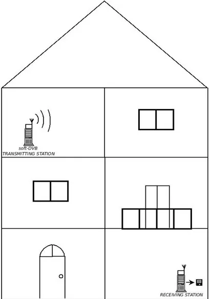
In the second acquisition scenario, as schematically shown in Fig. 2.7, the transmitting station is set at the second floor of a building while the receiving equipment at the ground floor. The stations now are distant several meters. Scenario is NLOS and there are a lot of walls and metallic materials between the stations. Leaving unchanged the tx gain at 0 dB, the rx gain varies from 26 dB to 30 dB.

In Fig. 2.8 and Fig. 2.9 are shown the PSD of the acquired signal respectively for rx gain 27 dB and 30 dB.

Fig. 2.8 – PSD of the acquired signal with rx gain of 27dB in the second scenario

As shown in figures, independently from the acquisition scenario the increase in the gain causes a substantial rise of the OFDM spectrum over the noise floor which is visible as fluctuations of the virtual carriers which should be null. This fluctuation of the virtual carriers will be used to implement the Minimum Mean Square Error (MMSE) channel equalization, as described in 3.9.2.

It can be interesting to compare the two different scenarios at fixed rx gain. It is possible to observe that, both at 27dB and 30dB, the SNR is lower in the second scenario.

2.2

8k mode

The most charming challenge of this work was maybe the possibility to receive and demodulate a DVB-T signal transmitted from one of the several broadcasters present on the Italian digital television market. Almost all of these transmissions use the 8k mode in order to satisfy the necessity to have a dense channel estimation, thanks to the large number of scattered and continual pilot carriers, and therefore afford an higher bit-rate by using a larger signal constellation (64-QAM).

2.2.1 Below-Nyquist reception, just a little bit...

The title of this subparagraph seems to be an absurdity. In fact, it is well known as it is impossible to represent completely an analogue signal with a digital one without respecting the Nyquist-bound that is sampling a signal with a sampling rate lower than the signal-bandwidth multiplied by 2.

The 8k mode signal transmitted by the broadcasters has a baud rate of 64/7 complex Msamples/s on a 64/7 MHz channel bandwidth, cyclic prefix length of 1/32 and 64-QAM constellation. As seen above, the maximum rate possible on USB interface is 8 complex Msamples/s.

By theory it is impossible to represent the DVB-T signal with a digital stream with a rate of 8 complex Msamples/s. However the specific features of the DVB-T spectrum makes possible the impossible. In fact, thanks to the presence of virtual carriers, the information carried by DVB-T signal is contained in a bandwidth smaller than 64/7 MHz so that there is no aliasing and no information-loss in sampling at a rate of 8 complex Msamples/s.

Assuming that there is no information loss, the problem is to represent at the receiver the signal formatted as described in ETSI standard, i.e. one sample every 7/64 of a μ-second, in order to demodulate correctly the video stream. The solution to this

problem is to perform a rational resampling of the signal before doing any processing on it. The functional blocks of the rational resampler will be shown in 3.2. The rational sampling factor is 7/8 so that:

8 MSamples/s∗7 8=

64

7 Msamples/s Eq.2.1

Now it can be possible to understand the absurd title of this subparagraph. In fact, thanks to the resampler and the particular form of DVB-T spectrum, it is possible to demodulate the signal just a little bit below Nyquist-reception.

The only remaining problem is the presence of a relative and constant drift between the DAC of the transmitted signal at a rate of 64/7 MSamples/s and the ADC of USRP at rate of 8 Msamples/s. This effect could cause loss of synchronization approximately every three DVB-T frames which are composed by 68 OFDM symbols. Therefore, synchronization tracking strategy hat to take such impairment into account. 2.2.2 Acquisition scenarios and hi-SNR acquisition near Monte Serra

In 8k mode, differently from 2k mode, was not possible to have a perfect dump to test the sync-chain at fixed, controlled SNR. For this reason it is necessary to choose acquisition scenarios characterized by high SNRs, to have the possibility to measure the SNR, for example with an hardware receiver, and to implement an SNR estimation algorithm to compare the SNRs and to quantify the noisiness of the sync-chain and of the USRP hardware.

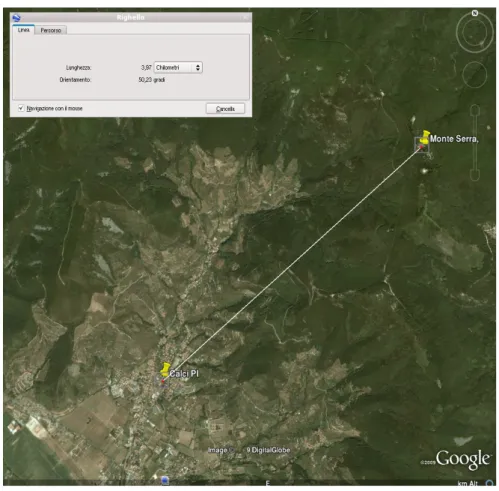
In most of Tuscany region DVB-T signal is broadcast by the antennas placed at the top of Monte Serra, near Pisa. In fact, the geographical position of the mount makes it proper to a broadcast service like DVB-T, as shown in Fig. 2.10 and Fig. 2.11. The acquired signal is on channel 56 with central frequency on 754 Mhz.

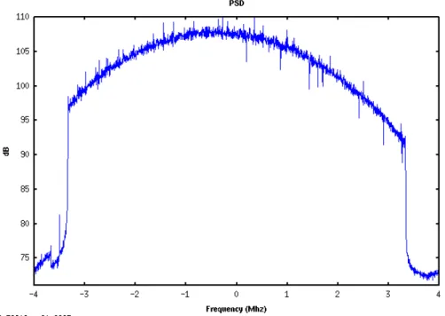
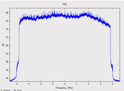
The first acquisition scenario it is a fixed receiving station in Pisa in LOS with Monte Serra at a distance of about 13 Km, as explained by Fig. 2.12. Fig. 2.13 shows

the PSD of the acquired signal. Some spikes are visible in the spectrum on a quasi-AWGN channel.

Fig. 2.10 – Antennas on Monte Serra

Fig. 2.12 – Distance between Pisa and Monte Serra, source: Google Earth

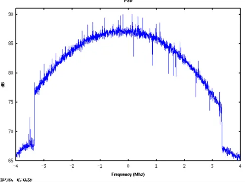
In the second scenario the fixed receiving station is collocated in Calci (PI) at a distance of about 4 Km from Monte Serra. As shown in Fig. 2.15 the signal-SNR is higher than before. Nevertheless channel-selectivity is more visible due to the presence of numerous hills which cause multi-path propagation.

Fig. 2.15 – PSD of the acquired signal in Calci (PI)

In order to acquire a signal with an higher SNR, a special acquisition setup was developed and used, which can be mounted on a car and powered by a car-lighter. The setup consists of:

• one splitter for the car-ligther;

• two DC-DC converters to power the capturing PC and the USRP;

• one capturing PC with a Remote Desktop (Virtual Network Computing-VNC)

Server;

• one USRP;

• one antenna;

• one netbook PC powered by battery with a VNC client to control the system.

A complete scheme of the setup is shown in Fig. 2.16.

Thanks to this mobile setup it has been possible to look for a signal with good SNR in order to optimize the demodulation. Fig. 2.18-20 show the real application of

Fig. 2.16 – Mobile acquisition setup

The PSD of the acquired signal is shown in Fig. 2.21. It is interesting to note an higher SNR and a quasi-AWGN channel so that this acquisition represents a perfect test for the sync-chain. In fact, as described in 5.3, this is the first 8k mode video that the fully software receiver was able to demodulate.

Synchronization chain blocks

This chapter describes the blocks of the implemented sync-chain both for 2k and 8k mode focusing on their implementation and computation complexity. It is shown how block-implementation has been always guided by experimental results.

3.1

Sync-chain block diagram

3.2

Resampler in 8k mode: a fundamental step to receive 8k mode

signal

As shown in 2.2.1, in 8k mode in order to demodulate signal, it is necessary to resample the input stream, captured at complex 8 MSample/s up to complex 64/7 MSample/s so resulting in a rational resampling rate of 8/7.

Before any operation it is necessary to cast the acquired samples from signed short int (2 byte) to float (4 byte) through an explicit casting and to put them in a specific C++ class (complex.h) which deals with the complex items and implements the common operations (+, -, *, /, abs(...), arg(...)) being defined on the complex numbers.

As shown in Fig. 3.2, the resampling operation is performed in 3 steps:

● zero padded upsampling with rate = 8;

● filtering with a low-pass Finite Impulse Response (FIR) filter; ● downsampling with rate = 7.

Fig. 3.2 – Resampler block diagram

The most important step of this process is the design of the low-pass filter. It is a FIR filter working at a frequency of 64 MS/s.

The time domain implementation of the resampling block is computationally expensive as it yields numerical convolution. So, in order to reach real-time goal, it is necessary to optimize this operation. For example, it is possible to implement the filtering in frequency-domain by using the optimized FFT and IFFT algorithms described in 3.6.

3.3

Automatic Gain Control (AGC)

The next block in the sync-chain is an AGC. This block is necessary both to fix the sample-dynamics and prevent rapid change of SNR which can provoke the lack of the synchronization.

This operation is performed on each OFDM symbol (N complex samples, 2048 in 2k mode and 8192 in 8k mode) by computing the power Pk of the acquired k-th

OFDM symbol (Eq. 3.1) and then dividing each sample Sik by the square root of the

measured power (Eq. 3.2) so that the resulting signal is characterized by unitary power. P_k=

∑

∣

_∣



3.4

Timing and fractional frequency offset estimation

In a receiver the estimation of arrival time of the OFDM symbol and of frequency offset between local oscillator and the transmitter's one is fundamental in order to correctly demodulate the signal. The ambiguity on the arrival time causes a rotation of the data symbols while the frequency offset generates a shift of all subcarriers. In 3.4.1 an efficient open-loop algorithm to estimate these parameters is described while 3.4.2 shows the integration of this algorithm into our thesis work and the choice of project variables which optimize it.

3.4.1 Borjesson algorithm: an efficient open-loop algorithm

Borjesson's algorithm [6] implements a Maximum Likelihood (ML) timing and fractional frequency-offset estimator by exploiting the inner redundant information contained in cyclic prefix. It is assumed that the cyclic prefix length it is known and the transmitted signal s(k) is affected only by complex additive white Gaussian noise (AWGN) n(k).

As described in 1.4 and in Fig. 3.3, in OFDM in order to avoid Intersymbol Interference (ISI) and preserve orthogonality between subcarriers, the last L samples of the body of OFDM symbol (N samples long) are appended as a preamble to form the complete OFDM symbol (N+L samples long). The presence of the cyclic prefix makes also the signal pseudo-periodical so that errors in timing estimation cause only a constant phase-rotation of all the subcarriers in frequency domain. The possible value of L are expressed as a fraction of N (eg. N/4, N/8, N/16, N/32). Soft-DVB transmits a 2k mode signal with L = N/4 = 2048/4 = 512 while the signal transmitted from Monte Serra is an 8k mode signal with L = N/32 = 8192/32 = 256.

Fig. 3.3 – Structure of OFDM signal with cyclically extended symbols s(k)

The received signal r(k) can be represented as:

where θ is the integer-valued unknown arrival time and ε is the frequency offset between transmitter and receiver oscillators as a fraction of the intercarrier spacing (Δf = 64/7 MHz / 8192 = 1116 Hz in 8k mode, Δf = 8 MHz/2048 = 3906 Hz in 2k mode).

If it is assumed that data symbols xk are independent, s(k) is a linear

combination of independent and identically distributed random variables so that, thanks to the central limit theorem, s(k) can be approximated with a complex Gaussian process whose real and imaginary part are independent. This process in not white because of the inner correlation in the OFDM symbol generated by the insertion of cyclic prefix.

In a synchronizer the time error requirements may range from the order of one sample (wireless application, channel phase tracking) to a fraction of a sample (high bit- rate digital subscriber line).

The effect of the frequency offset is a loss of orthogonality between the subcarriers and the rise of the Intercarrier Interference (ICI) so that the effective SNRe

is lower bounded by r  k =s k − ej2 k/ Nn k  Eq. .3 3 SNRe SNR 1 .0 5947SNR sin2  sin     2 Eq. .22

where SNR=s 2 /n 2 , s 2 =E {

∣

∣

∣

∣

The sensitivity to a frequency offset ε is measured by the difference between SNR and SNRe. In absence of additive noise to obtain SNRe = 30 dB it is necessary

that ∣∣1.3⋅10−2 .

In the algorithm 2N + L samples, which contain one complete (N+L) sample long OFDM symbol, are collected in a (2N + L) x 1-vector r.

The log-likelihood function, as described in [6], under the assumption that r is a jointly Gaussian vector can be written as:

where

The first term in Eq. 3.5 is the weighted magnitude of  , which is a sum of L consecutive between pairs of samples spaced N samples apart. The weighting factor depends on the frequency offset. The term   , is an energy term independent of the frequency offset that depends on the SNR.

The maximization of the log-likelihood function can be performed in two steps:

The maximum with respect to the frequency offset ε is obtained when the cosine term in Eq. 3.5 equals one. The ML estimation of ε is

where n is an integer value which represents the integer frequency offset as integer multiple of the intercarrier spacing. At this step n = 0 is assumed because the

m=

_∑

∑

∣



∣

_∣

∣

_∣

∣

estimation and correction of integer frequency offset is performed in subsequent blocks. By using the ML estimation of ε, the log-likelihood function becomes

The joint ML estimation of θ and ε becomes

In absence of noise, the peak-value of the log-likelihood function is 0. The only two quantities affecting the log-likelihood function and the performance of the estimator are the length L of the cyclic prefix, which is assumed as known, and the correlation coefficient ρ given by the SNR and fixed at 1 in this thesis according to the operating SNRs of DVB-T standard that make ρ very close to 1. The structure of the original algorithm is shown in Fig. 3.4.

Fig. 3.4 – Structure of Borjesson estimator

, _ML=∣∣− . Eq.3.10 _ML=arg max  {∣∣− } Eq. 3.11 _ML=− 1 2arg  . Eq.3.12

Fig. 3.5-10 show some realizations of log-likelihood function , _ML

for different value of N and L in order to show the importance of the a-priori knowledge of signal parameters N and L that in this case are respectively 8192 and 256.

Fig. 3.7 – Log-likelihood function , _ML with N = 8192 and L = 2048

Fig. 3.9 – Log-likelihood function , _ML with N = 8192 and L = 512

As expected, the better the values of N and L are estimated the more the log-likelihood function peaks stand clearly above the noise floor with peak-values close to the theoretical perfect value 0.

3.4.2 System design: adaptation and choice of project variables

In order to reach the complete and correct demodulation of the signal, the original Borjesson algorithm is not enough accurate even if it is the core of this synchronization block.

In fact, some inner assumptions of the algorithm about the parameters θ and ε are not true in a real world signal acquisition. For example, the real frequency offset is not only a fraction of the intercarrier spacing but can assume values of several intercarrier spacing and also varies slowly during the estimation-time. Fig. 3.11 shows a realization of the log-likelihood function , _ML calculated on a 8k mode acquired signal with estimated SNR of about 18 dB.

In order to expand the gap between the peak-values and the noise floor and obtain an accurate estimation of the parameters also at the lowest SNR covered by the standard an average operation among adjacent realizations of the log-likelihood function has been performed. The number of realizations Ns to be averaged represents,

for the sync-chain, a design variable. Fig. 3.12-14 represent the averaged log-likelihood functions for different numbers of averaged realizations (Ns = 10, 100,

200).

Fig. 3.12 – Averaged log-likelihood function , _ML (SNR ~ 18 dB), Ns = 10

It is important to note the improvement achieved in the estimation precision by averaging even just 10 realizations. The noise floor has a limited dynamics, the gap between the peak value and the noise floor is bigger and the width of the peak is reduced so producing a more accurate estimation of the arrival time θ and consequently of fractional frequency offset ε.

Fig. 3.13 – Averaged log-likelihood function , _ML (SNR ~ 18 dB), Ns = 100

By increasing Ns the dynamics of noise floor is further limited but the width of

the peak is larger than the previous case (Ns = 10). This effect is caused by the

presence of constant drift in the 8k acquired signal. In fact, by observing the averaged log-likelihood function on numerous adjacent realizations (Ns = 100, 200), it can be

noted that peaks do drifts so that averaging several realizations the resulting averaged peak is larger. Furthermore the computational complexity of the algorithm grows linearly with Ns so that it is necessary to choose a low value for Ns. In the sync-chain

implemented within this thesis, Ns has been fixed at 10 as result of this trade-off.

Thanks to this adaptation of the algorithm, it is possible to obtain accurate estimation also at the lowest SNRs assumed in the ETSI DVB-T standard. Fig. 3.15-18 show some realizations of the log-likelihood function at different values of Ns for

an 8k acquired signal at low SNR (~ 16 dB).

Fig. 3.15 – Log-likelihood function , _ML (SNR ~ 16 dB), Ns = 1

By using Ns = 1 it is impossible to reveal the position of the autocorrelation

Fig. 3.16 – Log-likelihood function , _ML (SNR ~ 16 dB), Ns = 10

Fig. 3.18 – Log-likelihood function , _ML (SNR ~ 16 dB), Ns = 200

By using Ns = 10 the peak is clearly visible so that an accurate estimation is

performed. Note that this is the only way to obtain a more accurate estimation through Borjesson algorithm. For Ns = 100 and Ns = 200 the previous considerations about the

width of the peak and the dynamics of the noise floor are valid. Note that, being SNR = 16 dB already under the SNR required by the standard for the used mode, this result supports the choice of Ns = 10.

In order to show the trend of the fractional frequency offset during the acquisition and to characterize the behavior of USPR local oscillator, the estimation has been performed every 500 OFDM symbols by using Ns = 10. The used signal is

an 8k mode with SNR ~ 18 dB. The resulting temporal trend is shown in Fig. 3.19. It can be noted that, during the acquisition, the fractional frequency offset grows quasi-linearly so that the local oscillator of USRP drift in excess with respect to the oscillator of the transmitting station. To understand this trend it is necessary to remember that ε represents only the fractional part of the offset so that when it

fractional offset. At this point of implementation, it was assumed that also the integer frequency offset varied during the acquisition and it was therefore necessary to recovery and correct it. These hypothesis will be verified in 3.7. An infinite drift of the frequency offset can not be true. In fact, in the last part of the acquisition it is possible to note a bend in the fractional frequency offset curve probably yielded by a decrease in the integer offset.

Fig. 3.19 – Timing trend of the fractional frequency offset (SNR ~ 18 dB, Ns = 10)

This estimation, being a computationally complex operation, is not performed at regular symbol intervals, as shown in Fig. 3.19, but only when the flag alignment is set to false by the threshold based alarm algorithm described in 3.11.

3.5

Alignment, cyclic-prefix removal and fractional frequency offset

correction

In this blocks, the previous estimations are used in order to correct in time domain both the timing and fractional frequency offset.

The alignment operation, as shown in Fig. 3.1, is performed only when the estimation of θ and ε is renewed, being the boolean flag alignment set to false. In this case a shift of  is performed in the reading data-index for aligning the signal to the beginning of an OFDM symbol. The aligned signal r_ak  can be written as

After the alignment to an OFDM symbol, the next block removes from the symbol the cyclic prefix samples, unnecessary to decode the signal. r_{sa , i}k 

represents the selected part of the i-th OFDM symbol r_{a , i}k  . where

ra , ik L=s i∗ N  Lk  L −ej2 i∗ N Lk L / Nni∗ N Lk L

The correction of the fractional frequency offset is performed after the removal of the cyclic prefix in order to do fewer operation by focusing the correction only on the useful samples at runtime. The correction is performed in time domain by multiplying each symbol for a complex exponential characterized by the estimated

 . The corrected i-th OFDM symbol r_{input ,i}k  can be written as

It is important to note that, differently from what happens for the alignment operation, the removal of cyclic prefix and the fractional frequency offset correction have to be performed for all the acquired OFDM symbols and so they have a direct influence on the execution time.

rak =r k  =sk  −e

j2  k  / N

n k . Eq.3.13

r_{sa , i}k =r_{a ,i}k L k=0,... ,  N −1 Eq.3.14

3.6

Fast Fourier Transform

As described in 1.4 the last block in the modulation chain before the insertion of the cyclic prefix is an IFFT, so that the dual block in the demodulation chain is an FFT which acts as a matched filter for OFDM modulation. The signal r_inputk  is the input of the FFT block. The size of the FFT is equal to N (8192 for 8k mode and 2048 for 2k mode) and performed symbol by symbol. The OFDM output symbol X_ik 

can be written as:

In order to reach the real-time goal it has been necessary to optimize this complex operation by using a C++ subroutine library, the “Fastest Fourier Transform in the West” (FFTW) version 3.2.2.

3.6.1 FFTW3: an open-source optimized FFT computation algorithm

FFTW3 is an open-source optimized FFT computation algorithm created and developed by Matteo Frigo and Steven G. Johnson at Massachusetts Institute of Technology (MIT). It is possible to compute the DFT in one or more dimensions, of arbitrary input size, and both for real and complex data set. It is possible to download the source package from the Internet site [7]. Additional information can be found in paper [8]. The performed benchmarks on several platforms have shown the superior performance of FFTW with respect to the other available open-source FFT and the competitiveness with vendor-tuned codes. For these features FFTW won the J. H. Wilkinson Prize for numerical software in 1999.

FFTW is optimized to work with data types like double (8 byte) and float (4 byte). In this thesis, FFTW is used with complex items whose real and imaginary part are represented by a float (4 byte).

To use FFTW is necessary to create a plan:

fftwf_plan fftwf_plan_dft_1d(int n, fftwf_complex *in, fftwf_complex *out, int sign, unsigned flags)

where n is the size of the FFT, in and out are pointers to the complex array of input and output data, sign indicates the direction of the transform (-1 = FFT, +1 = IFFT) and flags indicates which kind of optimization has to be performed.

Now it is possible to perform the FFT and successively destroy the created plan:

void fftwf_execute(const fftwf_plan plan); void fftwf_destroy_plan(fftwf_plan plan).

Besides it is necessary to include <fftw3.h> after <complex.h> and to link the library during compiling operation with -lfftw3f.

The output OFDM X_ik  can be still affected by a residual integer frequency offset so that it is necessary to estimate and correct it.

3.7

Integer residual frequency offset estimation and correction

The presence of an integer (multiple of intercarrier spacing) frequency offset in

X_ik  results in a rigid shift of subcarriers position in OFDM spectrum.

It is possible to estimate integer frequency offset by applying several closed loop algorithms but this requires a more complex implementation due to the presence of additional loop in the sync-chain. Instead of this, the aim of this thesis is the implementation of open loop algorithms.

3.7.1 Energy based estimation: an efficient open-loop algorithm

The energy based estimation of integer frequency offset is described in [9]. The core of this method is the use of a sliding window whose size is wide as the bandwidth occupied by the active subcarriers (6817 in 8k mode, 1705 in 2k mode). In a theoretical implementation, this windows slides over all the OFDM symbol calculating in each position the energy of the selected part, as shown in Fig. 3.20. The position in which the energy is the highest, represents the estimation of the integer frequency offset. The acquisition range of this estimation is large as the whole signal bandwidth. In order to obtain a good estimation also at low SNR it has been necessary to modify this algorithm by averaging several OFDM symbols in order to limit the influence of the noise and of the channel in the estimation. As the fractional frequency offset, the integer one varies during the acquisition so that sometimes it is necessary to repeat the estimation. In Fig. 3.21-23, the estimation is performed every 100, 300, and 500 OFDM symbols by using respectively 100, 300 and 500 OFDM symbols in the averaging operation at SNR ~ 16 dB.

Fig. 3.20 – Energy based integer frequency offset estimations (sliding window)

Fig. 3.22 – Integer frequency offset by averaging 300 OFDM symbols

Through the observation of the figures it has been decided to set the number of used OFDM symbols to 500.

The hypothesis with respect to the integer frequency offset, described in 3.42, are now demonstrated. In Fig. 3.24 fractional and integer estimated frequency offset are overlapped. The integer offset is normalized to 0 but actually his initial value is 2.

Fig. 3.24 – Frequency offset estimation (SNR ~ 16 dB)

In the implemented sync-chain, this estimation is not performed at regular intervals, as shown in the figures, but depends on the boolean flags alignment and

enough data. The first one is set by the alarm block while the second flag indicates if

enough data (500) is present in the buffer in order to perform a new estimation. Otherwise, the previous estimation is kept.

3.8

Channel estimation

As shown in chapter 1, in an OFDM system, the channel equalization is easier than it is in a traditional system because the information is contained within the frequency domain and, by inserting some subcarriers dedicated, it is possible to perform a good and robust channel estimation.

3.8.1 Continual and scattered boosted pilot

In ETSI DVB-T standard the active subcarriers are not all informative. In fact some subcarriers, called pilots, are transmitted at boosted power level in some positions of the OFDM symbol. These pilots are modulated according to a PRBS, shown in Fig. 3.25, whose polynomial generator is: X11 _{+ X}2 _{+ 1. The PRBS is}

initialized so that the first output PRBS bit coincides with the first active subcarrier. A new value of the sequence is generated by the PRBS on every used subcarrier (whether or not it is a pilot).

Fig. 3.25 – Generation of PRBS sequence

The modulation of pilots is given by:

where m is the frame index, l is the time index of the symbols, k is the frequency index of the carriers, wk is the k-th output PRBS bit and E {∣c∣2} is the mean square

value of the used signal constellation. As seen in previous chapters, in this thesis work, for 2k mode the signal constellation is a non-hierarchical 16-QAM (

E {∣c∣2}=10 ) while in 8k mode it is a non-hierarchical 64-QAM ( E {∣c∣2}=42 ). Boosted pilots are divided into continual and scattered pilots. The first one occur on all symbols in the same position. Fig. 3.26 is shown the locations of the continual pilots in the OFDM symbol.

Fig. 3.26 – Location of continual boosted pilot in the OFDM symbol

The scattered pilots are transmitted in different positions for each symbol. The location of scattered pilots is defined by:

where Kmin = 0, Kmax = 1704 or 6816 (2k mode or 8k mode) and l is the time index of the symbols. The locations of scattered pilots are shown in Fig. 3.27.

Fig. 3.27 – Location of scattered boosted pilot in OFDM frame

3.8.2 Channel profile extraction and linear rectangular interpolation

Given the absence of the phase recovery, the channel estimation must be performed on each symbol. The channel estimation is performed in two steps:

• extraction of channel profile through boosted pilot; • linear rectangular interpolation of the channel profile.

The extraction of the channel profile is given by:

where k assumes the value of the pilot-location and Y(k) is the nominal value of the pilots. It is so necessary to calculate the PRBS just one. Through the PRBS it is possible to compute the nominal value of the scattered and continual pilots. As shown for the scattered pilot-location equation, only four sets of values are possible and are cyclically used. These sets are stored within a matrix.

Now it is necessary to interpolate the channel profile obtained through the Eq. 3.19. The linear rectangular interpolation represents, at run-time, the easiest and cheapest interpolation way. In an OFDM symbol the number of pilots, continual and scattered, is constant. They are 175 in 2k transmission mode while in 8k transmission mode they are 700. Nevertheless, the distance dk between the k-th pilot and the

subsequent one is not constant so that the slope of the interpolating line is not fixed. It



H_ik =Xik 

is necessary to pre-compute and store the pilot distances in a matrix. The interpolating equation is given by:

where k is the subcarrier-index, c is the subcarrier-index increment and mk is the slope

of the straight line. It can be written as:

Fig. 3.28 is a zoom of a channel interpolation where it is possible to note the different distances between the pilots.

Fig. 3.28 – Zoom of a channel interpolation  H_ik c =m_k∗c H_ik  c∈[0 ;d_k] Eq.3.20 mk=  H_ik d_k− H_ik  dk . Eq. 3.21

Fig. 3.29-30 show the channel estimation (module and phase) for a 2k mode acquired signal.

Fig. 3.29 – Module of estimated channel (2k mode)

Fig. 3.31-32 show the channel estimation (module and phase) for a 8k mode acquired signal.

Fig. 3.31 – Module of estimated channel (8k mode)

3.9

Equalization

This paragraph describes how the information on the channel, obtained from the previous block, is used in order to equalize the OFDM symbol. In OFDM the equalization is simpler than traditional modulation because the information is carried within the frequency domain so that the equalization is only a subcarrier-wise multiplication by the equalization function. As with traditional systems two possible approach are presented: Zero-Forcing (ZF) and MMSE.

3.9.1 Zero-forcing (ZF) equalization

ZF approach in frequency domain simply tries to invert the channel. The equalization function Qi(k) is given by:

The i-th equalized OFDM symbol Zi(k) is given by:

With this equalization strategy, continual and scattered pilots are perfectly recovered in the equalized symbol and represent the milestones for the whole equalization. Fig. 3.33-34 show the signal constellation of a 2k mode signal before and after the ZF equalization. The constellation used in 2k mode signal is 16-QAM that it is clearly visible in the equalized constellation but it is not intelligible in Fig. 3.33. In the constellation, boosted pilots are all concentrated in two points on the real axis ±4/3∗



_

Q_ik = 1  H_ik  k ∈[0 ; N −1] Eq.3.22 Z_ik =X_ik ∗Q_ik =Xik   Hik  k ∈[0 ; N −1] Eq. 3.23

Fig. 3.33 – Pre-equalization signal constellation of a 2k mode signal (16-QAM)

3.9.2 Minimum Mean Square Error (MMSE) equalization

ZF approach is the simplest way to equalize the signal but has some drawbacks. The most important one is the noise-enhancement. In fact, if the estimated value of the channel is low, when the channel inversion is imposed, the thermal noise can be enhanced. This effect can be shown by:

where the term n_ik / H_ik  can reach high values and affects the correct de-mapping of the information symbol ci(k).

In order to avoid this it is possible to apply the MMSE approach which aims to find a function Qi(k) which minimizes the mean square error given by:

The function Qi(k) can be written as:

where H_ik  is substituted by H_ik  and w2 by w2 which is the estimated

noise power at the receiver.

MMSE equalization eliminates the noise-enhancement because the performance of the equalizer depends on the value of H_ik  . If H_ik  is big, the first term prevails at the denominator and the equalizer acts as a ZF equalizer. If



H_ik  is small the second term prevails and this prevents the noise-enhancement. The drawback of this method is the need to estimate the noise-power at the receiver. At this point a way to estimate the thermal noise power in the pre-equalized signal it was necessary .

Z_ik =X_ik  Hik  =c_ik ∗H_ik  Hik   nik   Hik  k ∈[0 ; N −1] Eq.3.24 MSE =E {

∣

∣

∣

∣

∣

_∣

3.9.2.1 Noise power estimation on the virtual carriers

It is possible to estimate the noise power on the virtual carriers. In fact the virtual subcarriers are set to zero on the standard in order to shape the spectrum. In an actual acquired signal they are not null and the reason of this is the presence of noise on these subcarriers. In 2k mode, the virtual subcarriers are 343 while in the 8k mode are 1375. It is possible to compute the mean square value on these subcarriers which can be assumed as a good estimation of the noise power. It is possible to extend the estimation to several OFDM symbols because the noise-power depends on the hardware and the channel profile is fix because the receiving station is fixed.

Fig. 3.35-3.36 show the signal constellation of an 8k mode signal (64-QAM) after a ZF and MMSE equalization respectively.

It has been experimentally tested, and it is clearly visible also in the figures, that MMSE approach does not improve the sharpness of the signal constellation. MMSE equalizer is more computationally complex than the ZF one and so it was not implemented in the final sync-chain.

3.10 Correlation of TPS carriers with a Dirac-comb

In order to develop an efficient tracking of the synchronization status it is necessary to choose a stable and perfectly controllable metrics.

At first, the boosted pilots before the equalization block have been used to create a suitable metric but the impossibility to forecast exactly the dynamics of the pilots suggests to go beyond the equalization blocks in order to obtain a good metric.

The use of all the boosted pilots in the channel estimation and equalization prevents us from using them as a metric after the equalization. Actually the pilots are completely recovered and the information about synchronization correctness are lost.

The only reference subcarriers that can be used are the TPS subcarriers. As seen in 1.4, TPS are inserted in the ODFM spectrum together with the boosted pilots. They carry the information about the signal: a synchronization word to perform the alignment to an OFDM frame, the transmission mode, the length of the cyclic prefix, the rate of the convolutional code and some parity check bits of a Bose Ray-Chaudhuri (BCH) code.

TPS subcarriers are transmitted at normal power, E {∣c∣2}=10 for 16-QAM and E {∣c∣2}=42 for 64-QAM, in fixed position in the OFDM symbol. The locations of TPS are shown in Fig. 3.37.

Fig. 3.37 – Locations of TPS subcarriers in the OFDM symbol

The number of TPS is different for 2k and 8k mode. In 2k mode they are 17 while in 8k mode they are 68. An OFDM symbol carries only an information bit whose value is decided at majority. The number of information bits carried by the TPS