Acoustic pipeline monitoring : theory and technology

(1)

POLITECNICO DI MILANO

DEPARTMENT OF ELECTRONICS INFORMATION AND BIOENGINEERING DOCTORAL PROGRAMME IN INFORMATION TECHNOLOGY

ACOUSTIC PIPELINE MONITORING: THEORY AND

TECHNOLOGY

Doctoral Dissertation of: Silvio Del Giudice

Supervisor:

Prof. Giancarlo Bernasconi Assistant Supervisor: Dr. Giuseppe Giunta

Tutor:

Prof. Andrea Monti Guarnieri The Chair of the Doctoral Program:

Prof. Carlo Fiorini

(2)

(3)

(4)

Acknowledgements

Since all the content and the results of this thesis have grown within research projects promoted and supported by eni spa, I certainly wish to thank the company and in particular Dr. Giuseppe Giunta, the project manager of Dionisio research project. I wish to thank also Aresys s.r.l. which contributed to the project with the software production and Solgeo s.r.l. with instrumentation and services.

(5)

I

Abstract

his thesis deals with monitoring of pipelines through acoustic measurements. Acoustic monitoring is a technique that exploits the fact that any disturbance occurring in the pipe infrastructure or in the conveyed fluid produces or influences acoustic transients which propagate as waves within the fluid at distances of many kilometers, carrying information on the originating event and on the propagation channel.

I first analyze the theory of elastic wave propagation in pipelines and present a suitable matrix method to compute propagation parameters in fluid-filled pipelines possibly buried or submerged, taking into account several propagation effects among which fluid thermo-viscosity, pipe elasticity, external load and radiation.

The propagation parameters can be found at any frequency and for any axisymmetric propagation mode.

The theoretical study was functional to the design and development of a registered technology (e-vpms®) for pipeline monitoring which I contributed to.

This system in fact employs a discrete network of vibro-acoustic monitoring stations mounted along gas or liquid pipelines which measure synchronized physical signals. Thanks to measurements performed on a buried in-service oil pipeline, I have experimentally validated the propagation method presented in the whole range of frequency of interest.

Propagation parameters of acoustic waves were also measured in many in-service gas pipelines and found in agreement with theory.

An important application of the monitoring system is the leak detection system that was tuned and validated on an in–service oil pipeline.

In gas pipelines instead I describe some methods of pig (pipeline inspection gauge) tracking and a successful application of acoustic reflectometry on a pipeline to find and characterize anomalous pipe sections.

Moreover I propose, through real examples, further advanced processing to measured and stored data such as the long term monitoring which allows to identify the standard operational conditions in a pipeline and therefore detect possible anomalous situations.

A last type of application concerns the use of theoretical models of wave propagation and of fluid properties to interpret the measurements and obtain further information on the conveyed fluid and the flow regime.

(6)

II

Sommario

uesta tesi riguarda il monitoraggio di linee di trasporto per mezzo di misure acustiche. Il monitoraggio acustico è una tecnica che sfrutta il fatto che qualsiasi disturbo che si verifica nell’infrastruttura di trasporto o nel fluido trasportato produce o influenza transienti acustici che si propagano come onde nel fluido a distanze anche di molti chilometri, traportando informazioni sull’evento originario e sul canale di propagazione.

Inizialmente analizzo la teoria della propagazione di onde elastiche e presento un metodo matriciale apposito, per calcolare i parametri di propagazione in condotte contenenti fluidi eventualmente sommerse o interrate, prendendo in considerazione diversi effetti di propagazione tra i quali termo-viscosità dei fluidi, elasticità del tubo, carico e radiazione esterni.

E’ possibile poi ottenere i parametri di propagazione a qualsiasi frequenza e per qualsiasi modo di propagazione assi-simmetrico.

Lo studio teorico è stato propedeutico alla progettazione e sviluppo di una tecnologia registrata (e-vpms®) per il monitoraggio di linee di trasporto a cui ho contribuito. Questo sistema infatti impiega una rete discreta di stazioni di monitoraggio montate su linee per gas o liquidi che misurano segnali fisici sincronizzati.

Grazie alle misure eseguite su una linea ad olio interrata e in funzione, ho validato sperimentalmente il metodo di propagazione presentato nell’intero intervallo di frequenze di interesse.

I parametri di propagazione delle onde acustiche sono stati misurati anche su diverse linee a gas in servizio e risultati in accordo con la teoria.

Un’importante applicazione del sistema di monitoraggio è il sistema di rilevazione di fuoriuscite che è stato messo a punto e validato su una linea ad olio in funzione.

Per linee a gas invece descrivo alcuni metodi di tracciamento di PIG (sonde di ispezione per linee di trasporto) e un’applicazione di successo di riflettometria acustica su una condotta per trovare e caratterizzare sezioni di tubo anomale.

Propongo inoltre, attraverso esempi concreti, ulteriori elaborazioni avanzate di dati misurati e immagazzinati come il monitoraggio a lungo termine che permette di identificare le condizioni operative standard di una condotta e dunque rilevare eventuali situazioni anomale.

Un ultimo tipo di applicazione prevede l’uso di modelli teorici di propagazione delle onde e delle proprietà dei fluidi per interpretare le misure e ottenere ulteriori informazioni sul fluido trasportato e il regime di flusso.

(7)

III

List of figures

Figure 1.1. Compression and rarefaction due to a travelling wave ... 5

Figure 1.2. Velocity profile along inner radius ... 6

Figure 1.3. Pipe external load and radiation. ... 7

Figure 2.1. Phase velocity and attenuation computed with Model 2 ... 17

Figure 2.6. Phase velocity and attenuation computed with all models. ... 20

Figure 2.7: Phase velocity (top) and attenuation (bottom) computed with all models, zoom at low frequencies... 21

Figure 3.1. Cross-section of the waveguide constituted by 3 layers: Internal, Shell and External. ... 23

Figure 3.2. Cylindrical coordinates. ... 24

Figure 3.3. Vector composition of wavenumber. ... 37

Figure 4.1. Dispersion curves taken from Long et al. [12], with superimposed dispersion curve computed by AXISYM-3L for a water-filled pipe immersed in water. ... 48

Figure 4.2. Dispersion and attenuation curves taken from Long et al. [12], with superimposed (colored) curves computed by AXISYM-3L for a buried water-filled pipe. ... 49

Figure 4.3. Dispersion and attenuation curves in a gas-filled pipe. ... 50

Figure 4.4. Dispersion and attenuation curves in a mercury-filled pipe taken from Baik et al. [16] with superimposed in red some results from AXISYM-3L. ... 52

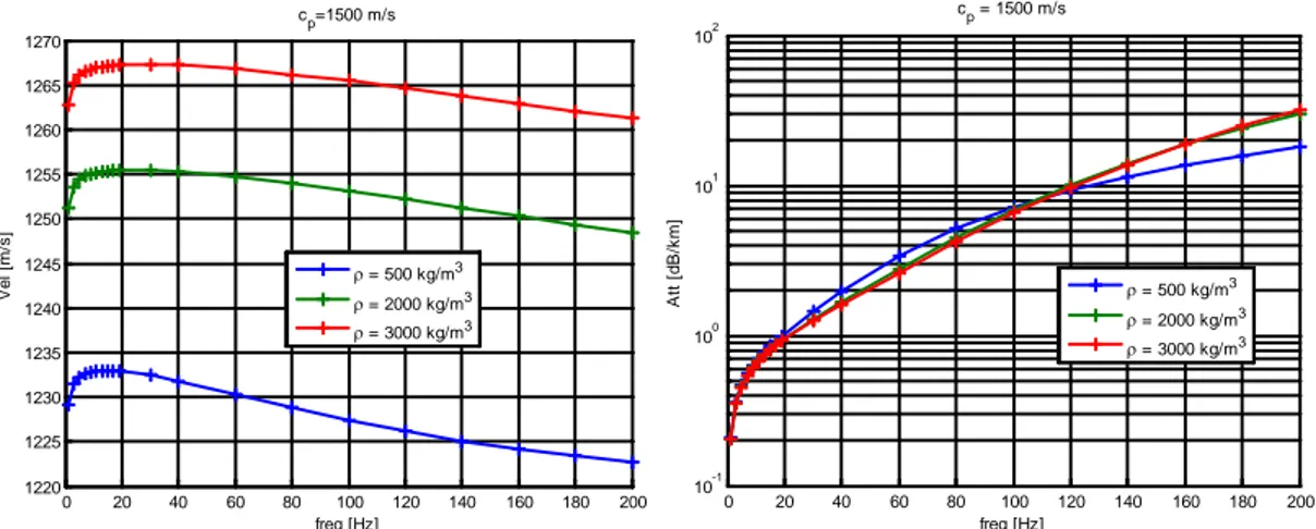
Figure 4.5. Phase velocity and attenuation for different values of surrounding medium density. External medium parameters are set as follows: cp=1500 m/s, cs=900 m/s. ... 53

Figure 4.6. Phase velocity and attenuation for different values of surrounding medium P-wave velocity. External medium parameters are set as follows: ρ=2000 kg/m3_, 3 / p s c c = ... 54

Figure 4.7. Phase velocity and attenuation for different surrounding media. ... 55

Figure 4.8. Phase velocity and attenuation computed with selected models. ... 56

Figure 4.9. Radial and axial displacements in a buried oil-filled pipe at 50 Hz. ... 57

Figure 4.10. Radial and axial displacements in a buried oil-filled pipe at 50 Hz.. Zoom around pipe. ... 58

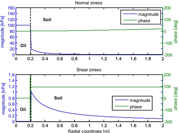
Figure 4.11. Normal and shear stresses in a buried oil-filled pipe at 50 Hz. ... 59

Figure 4.12. Normal and shear stresses in a buried oil-filled pipe at 50 Hz.. Zoom around pipe ... 60

Figure 1. e-vpms® vibroacoustic monitoring system. ... 63

Figure 5.1. Satellite map showing oil pipeline route (red line) and measurement stations (yellow dots) on the Chivasso-Pollein (Aosta) pipeline stretch. Three temporary measurements stations are in green. ... 66

(11)

VII

Figure 5.3. Scheme for estimation of response of the acoustic channel . Recording

stations in A, B, C, D, pump noise s0(t). ... 68

Figure 5.4. Reduction of pump noise from monitoring stations A and B. ... 69

Figure 5.5. Detection of leaks occurred between stations A and B ... 69

Figure 5.6. Acoustic pressure at Chivasso and VM21. Time signal (top), power spectral density (bottom). ... 71

Figure 5.7. Propagation from Chivasso to VM21. Cross-correlation of pressure signals. ... 72

Figure 5.8. Experimental wave attenuation ... 73

Figure 5.9. Attenuation curves measured and computed by models ... 75

Figure 5.10. Dispersion curves computed by models ... 76

Figure 5.11. Monitoring stations along Chivasso-Aosta pipeline. ... 77

Figure 5.12. Sound speed (top left) and pressure (bottom left) within the oil in the different pipe sections. Pressure/speed histogram in the first stretch (right) ... 78

Figure 5.13. Pressure - sound speed relation. Experimental data (dots) and Batzle and Wang (B-W) model [29]. ... 79

Figure 5.14. Attenuation-sound speed diagram. Theoretical models and experimental data (blue “areas”), measured in 2011. ... 81

Figure 5.15. Attenuation-sound speed diagram. Theoretical models and experimental data (blue “areas”), measured in 2012. ... 82

Figure 5.16. Pressure signal before pump replacement (May 11th, 2012). ... 82

Figure 5.17. Pressure signal after pump replacement (May 12th, 2012). ... 83

Figure 5.18. Pressure values distribution before and after pump replacement. ... 83

Figure 5.19. Frequency content of Chivasso pressure signal before (up) and after (bottom) pump replacement. ... 84

Figure 5.20. Autocorrelation of pressure signal at Chivasso station in December 2010. ... 85

Figure 5.21. Autocorrelation of pressure signal at Chivasso station in March 2011. 86 Figure 5.22. Autocorrelation of pressure signal at Chivasso station in March 2011. 86 Figure 5.23. Autocorrelation of pressure signal at Chivasso station in March 2011. 86 Figure 5.24. Autocorrelation of pressure at Chivasso station in December 2011. ... 87

Figure 5.25. Autocorrelation of pressure signal at Chivasso station, focus on travel time shift (left). Travel time from Chivasso to V28 stations in same time interval (right). ... 88

Figure 5.26. Pipeline scheme showing the position of the reflector, likely the highway. ... 88

Figure 5.27. Map showing the position of the intersection between pipeline and Milano-Torino highway. ... 89

Figure 5.28. Autocorrelation of pressure signal at Pollein station in December 2010. ... 89

Figure 5.29. Autocorrelation of pressure signal at Pollein station in March 2011. ... 90

Figure 5.32. Autocorrelation of pressure signal at Pollein station in December 2011. ... 91

Figure 5.33. Autocorrelation of pressure signal at Pollein station, focus on travel time shift (left). Travel time from Pollein to V35 stations in same time interval (right). ... 91

(12)

VIII

Figure 5.34. Pollein pressure signal(blue line) superposed to a scaled and delayed

copy of itself (red line). ... 92

Figure 6.1. TMPC TRANSMED pipelines ... 95

Figure 6.2. Phase 1: scheme of monitoring system ... 95

Figure 6.3. Phase 2: scheme of monitoring system ... 96

Figure 6.4. Satellite view: TMPC TRANSMED station of Mazara del Vallo (Italy) and sensor location. ... 96

Figure 6.5. Satellite view: TMPC TRANSMED station of Cap Bon (Tunisia) and sensor location. ... 97

Figure 6.6. Line L2S, Mazara del Vallo, pig arrival on 26th August 2009. ... 98

Figure 6.7. Line L2S, Mazara del Vallo. 5 Hz low pass pressure signal on 26th August 2009. GMT time. Vertical axis in Volts (10 kPa/Volt). ... 98

Figure 6.8. Line L2S, Mazara del Vallo. Pressure signal spectrogram on August 26 2009. GMT time. Explanation of pig-induced stationary waves. Time to distance conversion with an estimated sound velocity of 340 m/s. ... 99

Figure 6.9. Inspection pig (www.RosenInspection.net). ... 99

Figure 6.10. Acoustic pressure maxima on line L2S. Vertical axis in Volts (10kPa/Volt) ... 100

Figure 6.11. 5 Hz low pass pressure signal (absolute value on top, raw signal on bottom). Red circle indicates PIG1 damage. Vertical axis in Volts (10kPa/Volt). ... 101

Figure 6.12: PIG2 arrival, carrying fragments of previous damaged PIG1. ... 101

Figure 6.13. Pressure signal during PIG2 operation. Windows with increasing zoom factor. Vertical axis in Volts (10kPa/Volt). ... 102

Figure 6.14. PIG2 detection, with STA-LTA processing on pressure signal (horizontal axis 200s). ... 103

Figure 6.15. PIG2 pressure spectrogram. Pig distance around 5 km. ... 104

Figure 6.16. PIG2 pressure signal (top), acceleration on the pipe shell (center), velocity on the pipe shell (bottom). Pig distance around 5 km. Horizontal axis 200s. Vertical axis in Volts. ... 104

Figure 6.17: PIG2 signal at different distances (left) and power spectral density (right). ... 105

Figure 6.18. Experimental and theoretical attenuation coefficient ... 105

Figure 6.19. Block diagram of cross-correlation processing. ... 106

Figure 6.20. Cross-correlation of pressure signals measured at line terminals. ... 107

Figure 7.1. Satellite map of stretch A (Garlate), and summary of tests and installation. ... 109

Figure 7.2. Satellite map of stretch B, and summary of installation. ... 110

Figure 7.3. Example of data analysis. Spilling in V20, recording in V19: acoustic pressure within the fluid and acceleration on the pipe shell. ... 111

Figure 7.4. Attenuation of pressure waves in stretch A. Absolute pressure 5.2 bar. ... 112

Figure 7.5. Attenuation of pressure waves in stretch B. Absolute pressure 3.8 bar. ... 112

Figure 7.6. Satellite map of the pipeline route. ... 113

Figure 7.7. Pressure transients at V19, V20, V22, stations during an air spill test at V22. ... 114

Figure 7.8. Measured and computed pressure signals at V20 (top) and at V22 (bottom) ... 115

(13)

IX

Figure 7.9. Measured and computed pressure signals at V22 station. Zoom on echoes from P1, P2, P3 (top). Zoom on multiples of P1, P2, P3 (bottom).

... 116

Figure 8.1. CSM full-scale test pipeline map. ... 117

Figure 8.2 Acoustic pressure signal measured in the test pipe during spill. ... 118

Figure 8.3. PSD of pressure signal during spill test nr. 6. Lower 5 harmonics. ... 119

Figure 8.4. Experimental and theoretical (AGA10) speed of sound in natural gas. 120 Figure 9.1: offshore natural gas transportation Line 1 and Line 4. ... 121

Figure 9.2. Normalized cross-correlation between pressure signals at Messina and Favazzina, from 12:00 Feb 5th 2013 (bottom). Average cross-correlation (top). ... 122

Figure 9.3. Normalized cross-correlation between pressure signals at Messina and Palmi, from 12:00 Feb 5th 2013 (bottom). Average cross-correlation (top) ... 123

Figure A.1. Scheme of the one-dimensional waveguide used by the Transmittivity Method, the sun represents the source, triangles represent receivers. 126 Figure A.2 Notation for signals P that depart from or impinge to an interface. ... 128

(14)

X

List of tables

Table 2.1. Example scenario parameters ... 16

Table 2.2. Physical propagation phenomena considered by the models ... 22

Table 4.1. Parameters for test scenario. ... 50

Table 4.2. Elastic parameters of 3 different surrounding media. ... 55

Table 5.1. Stations along Chivasso-Aosta oil pipeline. ... 67

Table 5.2. Geometrical and media parameters ... 74

Table 5.3. Oil properties in GSB pipeline. ... 77

Table 5.4. Measured sound speed and background pressure. ... 78

Table 5.5. Model parameters for theoretical attenuation/sound-speed relation... 80

Table 6.1. TMPC pipeline: parameters of lines L1S and L2S. ... 94

Table 7.1. Main valves along the Passo Spluga pipeline, different colors distinguish stretches A and B. ... 108

Table 7.2. Minor anomalies in equivalent pipe model. ... 115

Table 8.1. Position of monitoring stations on CSM test pipe. ... 117

Table 8.2. Experimental speed of sound at CSM ... 119

(15)

XI

List of symbols

Latins

a External pipe radius

2 , 1

A unknown coefficients for P-waves in the pipe shell b Internal pipe radius

B Bulk modulus

2 , 1

B unknown coefficients for S-waves in the pipe shell

c Acoustic wave speed

2 , 1

C unknown coefficients for P-wave and S-wave in the internal layer

2 , 1

D unknown coefficients for P-wave and S-wave in the external layer

E Elastic modulus h Pipe wall thickness

) ( x

y

H Hankel function of x type, of order th y

j Imaginary unit

y

J Bessel function of 1st type, of order y

k Wavenumber

L Solution matrix for modal wavenumber

rad M Radiation mass P Pressure Pr Prandtl number rad R Radiation resistance r Pipe radial coordinate t time

T Temperature

y

Y Bessel function of 2nd type, of order y

z Impedance

Pipe axis coordinate Greeks

α Attenuation (per unit length) Pressure waves radial wavenumber

β Shear waves radial wavenumber γ Ratio of specific heats

ε Linear strain

Wavespeed correction factor

ζ Dynamic second (or bulk) viscosity η Dynamic shear viscosity

(16)

XII θ Pipe azimuthal coordinate

λ First Lamé parameter µ Second Lamé parameter ν Poisson ratio

ξ Modal wavenumber ρ Density

τ Stress

χ Pipe loss factor ω Angular frequency Subscripts f free-medium fluid n Mode number m External medium p Pipe Pressure wave ph Phase s Shear wave Superscripts E External layer I Internal layer r Radial S Shell (layer)

(17)

1

Framework and rationale

Nowadays pipelines are a widespread, efficient and cheap mean of transportation for many fluids, in particular hydrocarbons.

Possible failures or damages to such structures might cause serious economic, environmental and health consequences, that’s why it’s of paramount importance to monitor the working condition of pipelines.

In particular as regards to oil and gas pipelines, in many country the law compels fairly to install systems that detect leaks of a certain amount within a certain delay. Since conduits are often buried or laid on the sea-bottom it’s difficult to perform direct monitoring and there arose the need to think out techniques of indirect monitoring, often called non-invasive or non-destructive. Among these I can cite mass balance, Computational Pipeline Monitoring (CPM), even satellite surveillance. The technique dealt with in this thesis is acoustic monitoring which exploits the fact that many events to be monitored in the pipeline produce or influence acoustic transients and these propagate as waves within the transported fluid at distances of many kilometers, carrying information on the originating event and on the propagation channel.

During my PhD I contributed to the development of a vibro-acoustic monitoring system (e-vpms® registered technology) which employs sensors to measure acoustic and other signals to monitor pipelines.

The design and development of this technology have required the study of the theory of wave propagation in pipelines.

In the case of gas-filled pipelines, the pipe can usually be considered a rigid medium and the simple wide-tube approximation which describes the fluid-borne wave propagation (Blackstock [1]) is sufficient for most practical application, as claimed by Stecki & Davis [2]; in the case of liquids, the compressibility of the fluid is comparable to the compressibility of the pipe material and therefore the properties of the shell are important and possibly even the properties of the external medium. To this end, an interesting model is proposed by Pinnington and Briscoe [3] and extended by Muggleton [4], which accounts for pipe elasticity, and surrounding solid medium effects, but neglects fluid viscosity. In particular these authors show the large contribution to wave attenuation due to the outward radiation of both pressure and shear waves. The advantage of these models is their analytic form but their validity falls in proximity of the ring frequency.

In fact, in order to obtain solutions for all frequencies and all propagation modes, a more complex matrix method is needed, which was well described in Gazis [5]. More recently the matrix method was employed among others by Rama Rao and Vandiver [6] for propagation in boreholes, Sinha et al. [7] and Plona at al. [8] for fluid loaded pipes filled with inviscid fluid.

This approach has been generalized to any sequence of cylindrical elastic layers as the Global Matrix Method (Lowe [9]) and implemented in the Disperse software by Imperial College (Pavlakovic [10]); fluid layers are then treated as equivalent elastic

(18)

2

solid layers introducing the fluid viscosity by means of a fictitious shear wave (Aristegui et al. [11], Long et al. [12], Vogt at al. [13], Ma et al. [14]).

Elvira-Segura [15] also used a matrix method to couple an internal viscous fluid with an external solid layer surrounded by vacuum, this model was recently used and extended to viscous shells by Baik [16].

In Chapter 3 of this thesis, the formulation of Sinha et al. [7], which in turn borrows the formulation of Gazis [5], is used to model 3 cylindrical layers, where the core medium, is implemented as a solid but turned into thermo-viscous fluid by proper re-definition of Lamé parameters similarly to the Disperse software and Baik [16]. The method described, in general, allows to consider a waveguide made of 3 co-axial cylindrical layers each of which can be either solid or fluid. In case of solid it has an elastic behavior, described by elastic parameters such as Lamé’s, which could be even complex, like in [16]. In case of fluid medium, both thermal and viscous effects are considered, and for each of them, both the following types: bulk and boundary layer.

The switching from solid to fluid is easily performed by replacing Lamé parameters with proper functions of fluid’s viscous and thermal parameters.

In this way a unique model can be used for both gas- and liquid-filled pipelines, which can support technologies such as e-vpms®, for monitoring of pipelines in different ways like for example real-time remote detection of third-party interference or long-term monitoring of transportation efficiency or detection of malfunctioning, failures and anomalies along pipeline.

(19)

3

(20)

4

Introduction

I analyze here the theory of acoustic wave propagation as far as it is useful to describe propagation of waves that can be exploited for pipeline monitoring, considering both liquid and gas as filling fluids.

In the first chapter I qualitatively describe the wave propagation in pipes with particular care to the different phenomena of absorption and dispersion, mathematically modeled as propagation parameters, that take place in different scenarios of pipelines.

In Chapter 2 I report a selection of propagation models according to the phenomena they take into account, most of the models were selected for their relative simplicity, being analytic or semi-analytic. For each model the computation method is presented.

Then I choose a common scenario of particular interest to hydrocarbon transportation, that is a buried oil-filled pipeline, in order to compute and compare the results of the models presented.

The comparison shows that none of the methods presented can accurately compute the propagation parameters in the whole range of frequency of practical interest, at least from unit Hz up to hundred Hz, but a more general matrix method is needed. This general matrix method is called AXSYM-3L and is described in Chapter 3, it simulates a waveguide of 3 cylindrical layers where each layer can be set to solid or fluid; fluids are thermo-viscous.

In Chapter 4 I show some of the results of the model, limited to fluid-filled pipes, buried or submerged and to the fundamental fluid-borne propagation mode.

In particular I perform some tests to verify the effect of the surrounding media, and others to verify the effect of the thermal boundary layer.

Results of AXSYM-3L are shown in the scenario of Chapter 2 together with the other models, and AXSYM-3L looks suited to provide accurate results in a wider frequency range than other models.

Finally AXSYM-3L as a matrix method is used to compute and display also the profiles of field variables and these will be shown in physical units for the usual scenario at the typical frequency of 50 Hz.

(21)

5

1. Acoustic propagation in pipelines

Acoustic wave propagation in fluid filled pipes can be conveniently described by the dispersion curve, i.e. the dependence of the wave phase velocity on frequency and by the attenuation curve, i.e. the decay of the signal amplitude with propagation distance.

Dispersion and attenuation are complicated phenomena associated with 1. Fluid bulk viscosity and thermal conduction.

2. Fluid viscous and thermal interaction with the pipe wall. 3. Fluid relaxation.

4. Pipe visco-elasticity.

5. Pipe external load and radiation.

I give here a brief description and explanation of each of these effects.

1.1. Fluid bulk viscosity and thermal conduction

Bulk viscosity and bulk thermal conduction affect the propagation of any wave travelling in a fluid, both in guided propagation (e.g. within a pipe) and in free propagation.

The viscosity of the fluid resists to motion because of friction among fluid particles: this causes attenuation, because mechanical energy is converted to heat, and also velocity dispersion.

On the other side, during wave propagation, the particles of the medium are continuously compressed and expanded. Compressed particles get warmer than the expanded ones, and this temperature gradient gives rise to a heat flux from the hotter regions to the colder ones (Figure 1.1). The energy associated to the thermal flux is subtracted from the propagating wave energy, determining attenuation.

(22)

6

1.2. Fluid viscous and thermal interaction with the pipe wall

The pipe wall affects pressure wave propagation mainly in two ways: it causes additional shear stresses, and it exchanges heat with the fluid.

As regards to the first effect, the fluid particles adjacent to the pipe wall must be at rest (no-slip condition), whereas those near the pipe axis can move freely (Figure 1.2). A complex velocity profile establishes along the section: axial viscous shear stresses act on the fluid, determining absorption and dispersion.

Regarding the thermal effect, the pipe behaves as an infinite heat source at constant temperature. The motion close to the wall is isothermal, whereas the motion near the pipe axis is not isothermal. This produces again a complex temperature profile along the pipe section, a heat flux between particles, and therefore absorption and dispersion of the wave.

Figure 1.2. Velocity profile along inner radius

1.3. Fluid relaxation

Relaxation occurs in a chemically reactive fluid made up of more than one substance, or in a fluid made up of molecules whose internal energy is associated to different modes of molecules motion (translational, rotational and vibrational). When the equilibrium is modified by the passage of the wave, the different modes require different time periods to reset to the equilibrium values.

This circumstance produces wave attenuation.

1.4. Pipe visco-elasticity

If the pipe is not perfectly rigid, it tends to follow the disturbance propagating in the fluid by expanding and compressing. For a perfectly elastic pipe (including any external medium), no energy dissipation takes place, that is no wave absorption, but the wave velocity is reduced and dispersed.

On the other side, if the pipe is viscous, also absorption occurs, due to dissipation of energy during pipe deformation.

(23)

7

1.5. Pipe external load and radiation

If the pipe is surrounded by a medium different from vacuum, the properties of this medium can affect the wave traveling in the fluid (Figure 1.3).

First, in the same way as the pipe elasticity can reduce the wave-speed, the external medium contributes by changing the elasticity of the whole “waveguide system”. Second, the contact between the pipe and the external medium, which is assumed of infinite extent, allows the leakage of energy outwards, producing wave attenuation.

Figure 1.3. Pipe external load and radiation.

1.6. Discussion

For points 1 and 2, thermal and viscous effects are of the same order of magnitude only for gases, whereas in liquids thermal effects are negligible.

The bulk viscosity and bulk thermal effects are important only at ultrasonic frequencies or for very wide tubes, otherwise they are small compared to those due to the interaction with the pipe walls.

Relaxation can be important, for instance, in air and in sea water, but it is practically absent in fresh water. In air, the effect on absorption can be higher than the bulk thermo-viscous effects, but of the same order of magnitude, so that also relaxation is usually neglected in fluid-filled pipelines.

The pipe can be considered perfectly rigid when its Young modulus is much greater than the fluid bulk modulus, and/or when the pipe thickness is far greater than the radius: this is usually valid for gases, not for liquids.

ρ c

_p

c

(24)

8

The pipe viscous effect can be neglected for elastic materials, typically metals, while it is not negligible for other materials such as plastics, which are strongly viscoelastic.

Finally, the effect of the external medium is important only if it has a density comparable with the pipe’s density, and the pipe itself is not perfectly rigid. Therefore it becomes negligible when the external medium is gas, but it has to be considered for liquid filled elastic pipe surrounded by liquids or solids.

(25)

9

2. Literature review

Here I report the description of a selection of propagation models in fluid filled cylindrical pipelines. This review is not intended as an exhaustive state of the art, instead a set of representative models was chosen according to their scope and propagation effects accounted for with the purpose of analyzing separately the phenomena described in the previous section. The models will be presented approximately in increasing order of complexity and accuracy and their results will be shown and compared in a common scenario.

2.1. Literature models description

2.1.1. Model 1: water hammer

Reference: Liu [17] (pages 66-67) Framework

This model considers the celerity (speed) of water-hammer pressure waves in pipelines, from a hydraulic point of view. The water hammer generated by a sudden valve closure produces a high pressure variation and a significant expansion of the pipe wall, resulting in a reduction of wavespeed.

Assumptions

• (Implicitly) Axisymmetric wave motion.

• Low frequency, no dispersion nor attenuation is considered. • Inviscid fluid.

Computation procedure

The pressure wave speed c in the internal fluid is provided as a function of the free medium wavespeed c_f = B_f /ρ_f and the physical and geometric parameters of the fluid and the pipe.

ε ρ ) / 2 )( / ( 1 / h b E B B c f f f + = (2.1) f

B : fluid bulk modulus

f

ρ : fluid density

E : pipe Young modulus

b: internal pipe radius

h: pipe thickness

ε is a dimensionless factor equal to 1.0 when the pipe wall is thin (i.e., when 2b/h>25) while for thick-walled pipes (2b/h<25), the factor ε differs for different conditions, as follows:

(26)

10

Case 1. Pipeline anchored upstream

(

)

      − + + + = 2 1 2 2 1 ν ν ε h b b b h (2.2)

Case 2. Pipeline anchored against longitudinal movement

(

)

_      − + + + = 2 1 2 2 1 2 ν ν ε h b b b h (2.3)

Case 3. Pipeline with expansion joints throughout its length

(

)

h b b b h + + + = 2 2 1 ν ε (2.4)

where ν is the Poisson ratio of the pipe shell.

Notice that c is always less than cf, so the elasticity of the pipe walls has the effect

of reducing the wave speed.

2.1.2. Model 2: wide tube approximation

Reference: Blackstock [1] (pages 322-325) reporting results originally due to

Kirchhoff.

Framework

The model considers propagation of pressure waves in viscous fluids within rigid pipes. The model is applicable when the pipe rigidity is much higher than the fluid rigidity, like gases in metallic pipes.

Assumptions

• Axisymmetric wave motion.

• Rigid pipe (also elastic with suited addition). • Small amplitude pressure waves.

• Absorption is related only to interaction with the wall pipe, and it takes place in a narrow (with respect to the pipe radius) boundary layer. This condition is expressed as a double inequality for frequency, i.e. the model is valid for a limited frequency range (see [1] and [18])

The absorption coefficient

α

and the phase velocity cph are provided as functions

of the angular frequency ω, the pipe radius b, and the fluid physical properties (density ρ , speed of sound _f c_f, dynamic viscosity η, specific heats ratio γ and Prandtl numberPr ).

(27)

11       ₊ − = Pr 1 1 2 1 2 γ ρ ωη α f fc b (2.5)       ₊ − + = + = Pr 1 1 2 1 1 / 1 γ ω ρ η ω α f f f f ph b c c c c (2.6)

The absorption coefficient is proportional to the square root of frequency and to the inverse of the radius.

The phase velocity increases from 0 (at frequency 0) up to the free medium velocity (for infinite frequency).

The case of elastic pipe can be approximately considered by correcting, in both previous formulas, the free fluid velocity c_f, with the water hammer formula (2.1) (this is claimed by Stecki & Davis [2]).

2.1.3. Model 3: viscous incompressible fluid in elastic pipe

Reference: Morgan & Kiely [19]. Framework

The model focuses on propagation of pressure waves through liquid-filled flexible tubes. The fluid is considered viscous but incompressible, phase velocity and damping factor are functions of the viscosity of the liquid and of the internal damping in the tube wall.

Assumptions

• Thin walls.

• Small amplitude pressure waves.

• Pressure wavelength far greater than pipe radius.

• Speed of pressure wave in the fluid far less than compressional speed in pipe shell.

• Axisymmetric wave motion. • Incompressible viscous fluid.

The authors provide two different approximate solutions depending on the value of the parameter η ωρf b where f ρ : fluid density

η: fluid dynamic viscosity b: pipe radius

(28)

12

Case 1. Small viscosity: >>1 η ωρ_f b         _′ +       + − =               + − − = E E b Eh b b b Eh c f f f f ph 2 4 1 2 1 2 2 1 4 1 1 2 2 2 ω ν ν ω ρ η ρ ω α ω ρ η ν ν ρ (2.7)

Case 2. Large viscosity: <<1

η ωρ_f b       − ′ + ′ + − =       − ′ + ′ + − = ν ν ω ω ν ω ρ η ρ ω α ν ν ω ω ν η ω ρ ρ 4 5 2 2 1 4 5 1 2 4 5 2 2 1 4 5 1 2 E E b Eh b E E b b Eh c f f f f ph (2.8) ν: Poisson ratio. h: pipe thickness

E′ and ν′appear in case of pipe viscosity, that is when the elastic constants E and *

*

ν are complex because the stresses depend also on the strain rates. The following relations hold: ν ω ν ν ω ′ − = ′ − = j E j E E * * (2.9)

This model of pipe viscosity (Kelvin-Voigt) is actually not used for metals, therefore no values of E′ or ν′ are available for steel.

Please note that, by neglecting the pipe internal damping (or at low frequency), in both cases, the absorption coefficient has the same dependence on frequency as Model 2 (Blackstock [1]), while, for increasing

ω

,

α

gets a quadratic dependence on frequency.

Moreover, in the small viscosity solution, the phase velocity, not affected by internal damping, has a similar dependence on frequency as Model 2.

2.1.4. Model 4: inviscid fluid in elastic pipe surrounded by vacuum

(29)

13

Framework

The model considers the wave motion in a fluid-filled pipe in order to compare the analytical solution with measurements recorded on the pipe shell and in the fluid. Attenuation and dispersion curves are provided for the two axisymmetric wave modes associated with the longitudinal shell motion and the internal pressure wave. Here only the latter is reported.

Assumptions

• Frequency far less than ring frequency • Inviscid fluid

• Thin wall shell, pipe thickness far less than pipe radius • Fluid wavespeed far less than shell compressional wavespeed • Axisymmetric wave motion

• Pipe in vacuum

The propagation characteristic is defined through the wavenumber k₁ = /ω c_ph−iα

as a function of the free medium wavenumber k_f =ω/c_f.

        − + = h b Eh b B k k p f f 2 _ω2_ρ 2 2 1 / / 2 1 (2.10) p ρ : pipe density.

Since the wavenumber is real, no attenuation is accounted for, whereas the phase velocity coincides with Model 1, for low frequency (exactly at ω=0), then it slowly decreases.

2.1.5. Model 5: inviscid fluid in elastic, buried pipe

Reference: Muggleton et al. [4]. Framework

Authors consider the wave motion in a fluid-filled pipe, surrounded by an infinite elastic medium which can support both longitudinal and shear waves. The attenuation and dispersion curves are derived for two wave types (n=1,2), which correspond to a fluid dominated wave, and an axial shell wave. Here only the former is reported.

Assumptions

• Frequency far less than ring frequency • Inviscid fluid

• Thin wall shell, pipe thickness far less than pipe radius • Fluid wavespeed far less than shell compressional wavespeed • Axisymmetric wave motion

(30)

14

The propagation characteristic is defined through the wavenumber k₁ = /ω c_ph − jα

as a function of the free medium wavenumber k_f =ω/c_f.         + + + − + = ) / ( ) ( / / 2 1 ₂ ₂ ₂ 2 2 1 b Eh R j M h b Eh b B k k rad rad p f f _ω _ρ _ω _χ f f c k = ω (2.11)

With respect to the previous model 4, two additional phenomena are accounted for: the effect of the surrounding medium, and the internal pipe absorption. They appear in the wavenumber equation as three new terms

χ: the loss factor

rad M : radiation mass rad R : radiation resistance with ω / ) Im( ) Re( sn pn rad sn pn rad z z M z z R + = + = (2.12) pn

z and z are the impedances of the longitudinal and shear waves in the external _sn medium, for the two modes n=1,2. Here I deal just with n=1 (fluid-borne wave). Impedances are functions of the surrounding medium density ρ_m, and seismic wave velocities c and _p cs(respectively P- and S-waves)

) ( ) ( ) , ( ) 2 ( 0 ) , ( ) 2 ( 0 ) , ( ) , ( ) , ( ) , ( b k H b k H k k c j z _r n s p r n s p r n s p n s p s p m n s p ′ − = ρ (2.13) ) 2 ( 0

H is the zero order Hankel function of the second kind (for outgoing waves). The prime sign denotes differentiation with respect to the argument. k₍r_p_,_s₎_nare the radial components of the longitudinal and shear wavenumbers in the external medium, defined as

(

)

2 2 ) , ( 2 ) , ( ps n r n s p k k k = −

where k₍_p_,_s₎ are the longitudinal and shear wavenumbers in the external medium

n s p n s p c k ) , ( ) , ( ω =

Since the impedances in the external medium depend on k , which is the unknown ₁ solution, it must be found iteratively.

(31)

15

2.1.6. Model 6: viscous compressible fluid in elastic pipe

Reference: Elvira-Segura [15]. Framework

The method computes the velocity and the attenuation of an acoustic wave propagating inside a cylindrical elastic tube filled with a viscous liquid by means of a matrix technique. This allows to find exact solutions for any frequency and propagation mode, through a root-finding technique.

Assumptions

• Viscous fluid • Elastic pipe • Pipe in vacuum

• Axisymmetric wave motion

This model does not provide an analytic solution. It is a Matrix Method (MM) that has to be solved numerically.

The solutions for the complex wavenumber or complex frequency can be found by setting the determinant of the solution matrix to zero.

As a first step, the wave equations for the solid and the fluid are studied separately and the solutions for displacements as function of unknown coefficients are found. The solution matrix is built by imposing 3 boundary conditions to both pipe interfaces, resulting in a 6-by-6 matrix. For details see Reference.

The solution for the 1st fluid-borne mode can be found using the Wide-tube approximation as first guess and then searching in its neighborhoods.

2.2. Literature models example results

2.2.1. Scenario

I consider an oil filled steel pipeline, buried in an elastic medium. Model parameters are reported in Table 2.1.

Physical and geometrical parameters Symbol Value Unit Description Pipe geometry

b 0.2 m Pipe internal radius

h 0.0111 m Pipe thickness Internal fluid - Oil

f

ρ ₉₀₀ _kg/m3

(32)

16

f

c ₁₄₀₀ _m/s _{Speed of sound in free medium} f

B _1.8x109

Pa Bulk modulus (function of ρ and f cf)

η _1x10-2

Pas Dynamic viscosity

γ ₁ _- _{Specific heats ratio}

Pr Not used - Prandtl number Shell material – Steel

p ρ ₇₈₀₀ _kg/m3 Density E _2x1011 Pa Young modulus χ 0 - Loss factor

E′ ₀ _Pa _{Viscous term. See Eq. (2.9)}

ν _0.3 _- _{Poisson ratio} Surrounding medium m

ρ

₂₀₀₀ _kg/m3 Density p c ₁₅₀₀ _m/s _{P-wave speed} s c ₉₀₀ _m/s _{S-wave speed}

Table 2.1. Example scenario parameters

2.2.2. Model 1: water hammer

This model predicts a reduction of speed from 1400 to about 1220 m/s. 2.2.3. Model 2: elastic wide tube

Kirchhoff’s wide-tube approximation is modified to account for pipe elasticity, by correcting the free medium wave velocity with Model 1, Eq. (2.1). The resulting model will be referred to as “Elastic wide-tube”. Figure 2.1 shows phase velocity and attenuation computed with Model 2.

(33)

17

Figure 2.1. Phase velocity and attenuation computed with Model 2

2.2.4. Model 3: viscous incompressible fluid in elastic pipe

I use the solution for “Small viscosity”, as it appears to be satisfied in the whole frequency range. Figure 2.2 shows phase velocity and attenuation computed with Model 3.

2.2.5. Model 4: inviscid fluid in elastic pipe surrounded by vacuum Figure 2.3 shows phase velocity and attenuation computed with Model 4.

0 50 100 150 200 250 300 350 400 450 500 1160 1170 1180 1190 1200 1210 1220 freq (Hz) V e l (m /s ) 0 50 100 150 200 250 300 350 400 450 500 0 0.5 1 1.5 2 2.5 3 3.5 4 4.5 5 freq (Hz) A tt ( d B /k m ) 0 50 100 150 200 250 300 350 400 450 500 2390 2400 2410 2420 2430 2440 2450 2460 2470 2480 2490 freq (Hz) V e l (m /s ) 0 50 100 150 200 250 300 350 400 450 500 0 0.2 0.4 0.6 0.8 1 1.2 1.4 1.6 1.8 freq (Hz) A tt ( d B /k m )

(34)

18

2.2.6. Model 5: inviscid fluid in elastic, buried pipe

Figure 2.4 shows phase velocity and attenuation computed with Model 5.

2.2.7. Model 6: viscous compressible fluid in elastic pipe Figure 2.5 shows phase velocity and attenuation computed with Model 6.

0 50 100 150 200 250 300 350 400 450 500 1217 1217.5 1218 1218.5 1219 1219.5 1220 freq (Hz) V e l (m /s ) 0 50 100 150 200 250 300 350 400 450 500 -1 -0.8 -0.6 -0.4 -0.2 0 0.2 0.4 0.6 0.8 1 freq (Hz) A tt ( d B /k m ) 0 50 100 150 200 250 300 350 400 450 500 1190 1195 1200 1205 1210 1215 1220 freq (Hz) V e l (m /s ) 0 50 100 150 200 250 300 350 400 450 500 0 50 100 150 200 250 300 350 freq (Hz) A tt ( d B /k m )

(35)

19

0 50 100 150 200 250 300 350 400 450 500 1200 1202 1204 1206 1208 1210 1212 freq. [Hz] V e l (m /s ) 0 50 100 150 200 250 300 350 400 450 500 0 0.5 1 1.5 2 2.5 3 3.5 4 4.5 5 freq. [Hz] A tt [d B /k m ]

(36)

20

2.2.8. Model comparison

Figure 2.6. Phase velocity and attenuation computed with all models.

0 50 100 150 200 250 300 350 400 450 500 1200 1205 1210 1215 1220 1225 1230 freq (Hz) V e l (m /s ) M2, Elastic wide-tube M3, Morgan M4, Pinnington M5, Muggleton M6, Elvira-Segura 0 50 100 150 200 250 300 350 400 450 500 0 1 2 3 4 5 6 7 8 9 10 freq (Hz) A tt ( d B /k m ) M2, Elastic wide-tube M3, Morgan M4, Pinnington M5, Muggleton M6, Elvira-Segura

(37)

21

Figure 2.7: Phase velocity (top) and attenuation (bottom) computed with all models, zoom at low frequencies.

2.3. Discussion

Figure 2.6 and Figure 2.7 show different attenuation and dispersion curves for the same scenario. This can be explained by the different assumptions in the various models, summarized in Table 2.2. Model 1 doesn’t appear in the table because of its simplicity, but plays a role in Model 2.

0 5 10 15 20 25 30 35 40 45 50 1200 1205 1210 1215 1220 1225 1230 freq (Hz) V e l (m /s ) M2, Elastic wide-tube M3, Morgan M4, Pinnington M5, Muggleton M6, Elvira-Segura 0 5 10 15 20 25 30 35 40 45 50 0 0.5 1 1.5 freq (Hz) A tt ( d B /k m ) M2, Elastic wide-tube M3, Morgan M4, Pinnington M5, Muggleton M6, Elvira-Segura

(38)

22 Fluid compressibility Fluid viscosity Pipe elasticity Surrounding medium

Model 2 yes yes yes no

Model 3 no yes yes no

Model 4 yes no yes no

Model 5 yes no yes yes

Model 6 yes yes yes no

Table 2.2. Physical propagation phenomena considered by the models

Model 5 [4] is the only that takes into account the effect of the surrounding medium, which causes the attenuation to increase at high frequency.

Except for this phenomenon, the most general model is nr. 6 (Elvira-Segura [15]). Model 2 is similar to the latter, at least at low frequency, provided to replace the value of the free wave-speed with the velocity computed with water hammer model, Eq. (2.1), in both formulas for phase-velocity and attenuation.

At higher frequency the decreasing trend of the wave speed, due to the pipe elasticity, is the same in Model 6 and Model 4: the small scale difference should be due to the fact that Model 4 uses the water hammer approximation for null frequency, whereas model 6 should be more accurate.

Finally, since Model 3 considers the fluid to be incompressible, it clearly overestimates the velocity (which in fact falls outside the plot). This is reflected also in a lower attenuation, even if its trend resembles those of the other models at low frequency.

(39)

23

3. AXSYM-3L model description

None of the models described in the previous section takes into account simultaneously all the propagation phenomena that are really relevant in fluid-filled pipelines.

Another model would be “Disperse” by Imperial College, available as a commercial software, which includes all the phenomena listed in Chapter 1 except for the thermal effects which are important mainly in gas-filled pipelines. The method of Disperse is much more general than the models presented so far and therefore it is also more complicated.

Hence I have built a new model, simpler than Disperse though it can simulate also thermal effects, which for convenience is here called AXSYM-3L.

The new model is a matrix method as well and starts from the formulation (and the notation) of Sinha at al. [7], in particular it considers 3 cylindrical layers, the most external extends infinitely in the radial direction (Figure 3.1), and restricts to axisymmetric waves. These are the two reasons for the given name.

Figure 3.1. Cross-section of the waveguide constituted by 3 layers: Internal, Shell and External.

Unlike [7], all 3 layers are mathematically treated as (visco)-elastic solids and the solution is obtained, any solid layer can then be turned into a thermo-viscous fluid by redefining properly the Lamé parameters.

In the context of pipelines, the internal layer is typically a fluid, gas or liquid, the shell is always solid and the external layer might be solid, soil for instance, or fluid, water, air or even mud.

This model, as a matrix method, allows to compute the axisymmetric propagation modes of any order at any frequency, even if in this thesis only the fundamental fluid-borne mode is analyzed.

The main assumptions are:

• Longitudinally infinite and homogeneous waveguide • Homogeneous isotropic media

• No constraints outside the pipe, except for the presence of an external medium. • Axisymmetric propagation. b a + S L G b a + S E I

(40)

24

The following sections contain the complete derivation of the general model. As a first step, the mechanical wave equations are studied, and the solutions for displacements are found as a function of unknown coefficients. The solution matrix is built up by imposing four boundary conditions to both pipe interfaces, resulting in an 8-by-8 matrix. The solutions for the complex wavenumber can then be found by setting the determinant of the solution matrix to zero. This solution, which provides the propagation parameters, must be reached with numerical methods.

3.1. Wave equations

The wave equations in elastic materials can be drawn by solving a differential system where the following equations appear [7]:

• Equations of motion, Newton’s second law. • Constitutive equations (linking stress and strain). • Strain-displacement relations.

Figure 3.2. Cylindrical coordinates.

The equations of motion in cylindrical coordinates (Figure 3.2), are given by: z x y O P(r, θ, z) θ z x y O P(r, θ, z) θ

(41)

25          + ∂ ∂ + ∂ ∂ + ∂ ∂ = ∂ ∂ + ∂ ∂ + ∂ ∂ + ∂ ∂ = ∂ ∂ − + ∂ ∂ + ∂ ∂ + ∂ ∂ = ∂ ∂ r z r r t u r r z r t u r z r r t u rz zz z rz z r r z rr rz r rr r τ τ θ τ τ ρ τ τ τ θ τ ρ τ τ τ θ τ τ ρ θ θ θ θ θθ θ θθ θ 1 2 1 1 2 2 2 2 2 2 (3.1)

where

τ

_rr,

τ

_zz, τ_θθ, τ_r_θ , τ_z_θ,

τ

_rzare the stress components, u_r, u and _θ uz are the

displacement components and

ρ

is the mass density.

For a homogeneous, elastic and isotropic medium the constitutive equations are given by: z u u r r u r u_r _r _z rz rz z z r r zz zz rr rr ∂ ∂ + ∂ ∂ + + ∂ ∂ = ∆ = = = + ∆ = + ∆ = + ∆ = θ µε τ µε τ µε τ µε λ τ µε λ τ µε λ τ θ θ θ θ θ θθ θθ 1 2 2 2 2 2 2 (3.2)

where

ε

_rr,

ε

_zz, ε_θθ, ε_r_θ, ε_z_θ,

ε

_rz are the strain components, λ and µ are the Lamé constants.

The strain-displacement relations in cylindrical coordinates are given by:

      ∂ ∂ + ∂ ∂ =       ∂ ∂ + ∂ ∂ =       ₋ ∂ ∂ + ∂ ∂ = ∂ ∂ = + ∂ ∂ = ∂ ∂ = z u r u z u u r r u r u u r z u r u u r r u r z rz z z r r z zz r r rr 2 1 1 2 1 1 2 1 1 ε θ ε θ ε ε θ ε ε θ θ θ θ θ θ θθ (3.3)

(42)

26

The substitution of Eqs. (3.3) and (3.2) into Eqs. (3.1) gives the equations of motion with displacements as dependent variables.

If I consider the axisymmetric case only, the equations of motion are:

(

)

(

)

(

)

(

)

             ∂ ∂ + ∂ ∂ + ∂ ∂ + +       ∂ ∂ ∂ + ∂ ∂ + = ∂ ∂ ∂ ∂ + ∂ ∂ ∂ + +       − ∂ ∂ + ∂ ∂ + = ∂ ∂ r u r r u z u z r u z u r t u z u z r u r u r u r r u t u z z z r r z r z r r r r 1 2 1 1 2 2 2 2 2 2 2 2 2 2 2 2 2 2 2 2 µ µ λ µ λ ρ µ µ λ µ λ ρ (3.4)

3.2. Wave equations solution

The displacement components for axisymmetric waves in the shell layer S are derived by solving Eq. (3.4) [7]:

( )

[

]

[

( )

]

{

}

( )

[

]

[

( )

]

{

}

( )     + − + = + + + − = + + z t j S z z t j S r e B r Y B r J A r Y A r J j u e B r Y B r J j A r Y A r J u ξ ω ξ ω β β β α α ξ β β ξ α α α 2 0 1 0 2 0 1 0 2 1 1 1 2 1 1 1 (3.5) with 2 2 2 2 2 2 2 2 ξ ω β ξ ω α − = − = s p c c (3.6)

where cp and cs are the compressional and shear velocities in the pipe shell, ω is

the angular frequency, ξ is the mode wavenumber, A ,_i B_i are unknown coefficients,

( )

x

J_n and Y_n

( )

x are the Bessel functions of the first and second kind, respectively, of order n.

The displacement components in the internal layer I are derived from the same equations, but discarding those solutions that give an infinite value for r=0 (Bessel functions of second kind). I can write:

( )

{

}

( )

{

}

( )     − = + − = + + z t j I I I z z t j I I I I r e C r J C r J j u e C r J j C r J u ξ ω ξ ω β β α ξ β ξ α α 2 0 1 0 2 1 1 1 (3.7)

Similar reasoning holds for the external layer E, except that, since the layer is infinite radially, Bessel functions of second kind are not discarded but merged with Bessel function of first kind by means of Hankel functions

(43)

27

( )

{

}

( )

{

}

( )     − = + − = + + z t j E E E E z z t j E E E E r e D r H D r H j u e D r H j D r H u ξ ω ξ ω β β α ξ β ξ α α 2 ) 2 ( 0 1 ) 2 ( 0 2 ) 2 ( 1 1 ) 2 ( 1 (3.8)

whereC ,_i D_iare other unknown coefficients, Hn(2) are the Hankel functions of the

second kind and of order n.

2 2 ) , ( 2 2 ) , ( 2 2 ) , ( 2 2 ) , ( ξ ω β ξ ω α − = − = E I s E I E I p E I c c (3.9)

Caution must be taken to the selection of the correct root for α_E and β_E.

In fact the sign of these wavenumbers determines whether the wave mode radiates (is leaky) to the external medium or not; Muggleton et al. [4] among other authors (Junger, [20], Rama Rao & Vandiver [6], Long et al. [12]) claim that the guided wave may or may not radiate into the external medium depending on its wavespeed relative to the wavespeed in the surrounding medium.

The choice of the proper root will be treated in Section 3.6.

3.3. Boundary conditions

In order to find the solution of the propagation problem (displacements and stresses) in the waveguide constituted by the shell S, the internal core I and the external layer E, I need to find the constants of the motion present in Eqs. (3.5), (3.7) and (3.8) for S, I and E, respectively. The constants are obtained by imposing the boundary conditions to the pipe structure, whose section is depicted in Figure 3.1.

The boundary conditions are the same for both internal and external shell interfaces, but clearly apply to different media and positions:

Condition 1. _{( )} ( ) _{( )} a b E I rr a b S rr _, , , τ τ = Condition 2. _{( )} ( )_{( )} a b E I rz a b S rz _, , , τ τ = Condition 3. _{( )} ( ) _{( )} a b E I r a b S r u u , , , = Condition 4. _{( )} ( ) _{( )} a b E I z a b S z u u , , , = (3.10)

The previous equations describe the continuity of the radial stress τ_rr, of the shear stress τ_rz, and of the radial and tangential displacements, u_r and u_z, at the interfaces of radial coordinate equal to b and a.

Acoustic pipeline monitoring : theory and technology