Computational study of resting state network dynamics

(1)

Scuola di Scienze

Dipartimento di Fisica e Astronomia Corso di Laurea in Fisica

Computational study of resting state network

dynamics

Relatore:

Prof. Gastone Castellani

Presentata da: Daniele Corradini

Sessione II

(2)

“When we take a general view of the wonderful stream of our consciousness, what strikes us first is the different pace of its parts. Like a bird’s life, it seems to be made of an alternation of flights and perchings.”

(3)

Abstract

Lo scopo di questa tesi è quello di mostrare, attraverso una simulazione con il soft-ware The Virtual Brain, le più importanti proprietà della dinamica cerebrale durante il resting state, ovvero quando non si è coinvolti in nessun compito preciso e non si è sottoposti a nessuno stimolo particolare. Si comincia con lo spiegare cos’è il rest-ing state attraverso una breve revisione storica della sua scoperta, quindi si passano in rassegna alcuni metodi sperimentali utilizzati nell’analisi dell’attività cerebrale, per poi evidenziare la differenza tra connettività strutturale e funzionale. In seguito, si riassumono brevemente i concetti dei sistemi dinamici, teoria indispensabile per capire un sistema complesso come il cervello. Nel capitolo successivo, attraverso un approccio ‘bottom-up’, si illustrano sotto il profilo biologico le principali strut-ture del sistema nervoso, dal neurone alla corteccia cerebrale. Tutto ciò viene spie-gato anche dal punto di vista dei sistemi dinamici, illustrando il pionieristico mod-ello di Hodgkin-Huxley e poi il concetto di dinamica di popolazione. Dopo questa prima parte preliminare si entra nel dettaglio della simulazione. Prima di tutto si danno maggiori informazioni sul software The Virtual Brain, si definisce il modello di network del resting state utilizzato nella simulazione e si descrive il ‘connettoma’ adoperato. Successivamente vengono mostrati i risultati dell’analisi svolta sui dati ricavati, dai quali si mostra come la criticità e il rumore svolgano un ruolo chiave nell’emergenza di questa attività di fondo del cervello. Questi risultati vengono poi confrontati con le più importanti e recenti ricerche in questo ambito, le quali con-fermano i risultati del nostro lavoro. Infine, si riportano brevemente le conseguenze che porterebbe in campo medico e clinico una piena comprensione del fenomeno del resting state e la possibilità di virtualizzare l’attività cerebrale.

(4)

(5)

Introduction

It has been appreciated for at least two millennia that the brains of humans exhibit ongoing activity regardless of the presence or absence of any observable behaviours. As noted by Seneca in 60 A.D., “The fact that the body is lying down is no reason for sup-posing that the mind is at peace. Rest is... far from restful” (Seneca, 1969). Given the apparently contradictory characterization of “rest” it is prudent to begin with a def-inition. In the context of experimentation, “rest” is an operational definition refer-ring to a constant condition without imposed stimuli or other behaviourally salient events [13]. However, interest in the interplay between the intrinsic activity of the brain and the external world has seen a revival over the past decade, especially in neuroimaging. In fact, an assumption in many of the early studies was that such intrinsic brain activity is irrelevant and sufficiently random that it averages out in statistical analysis. However, despite the most elegant experimental designs, there were consistent patterns of deactivation that often accompanied increased cognitive demands. Hence, several researchers began to examine these deactivations based on the idea that the low-level baseline tasks were active states and that the patterns of activation and deactivation represented a shift in the balance from a focus on the internal state of the subject and its ruminations, to one on the external environment [15]. Numerous experimental investigations have shown that spontaneous brain ac-tivity during rest is highly structured into characteristic spatio-temporal patterns, the so-called resting-state networks (RSNs). The observation that there are relatively consistent distributed patterns of activity during rest led to the suggestion that it might be possible to characterize network dynamics without needing an explicit task to drive brain activity. This possibility has been explored in studies of RSNs in functional magnetic resonance imaging (fMRI). It has seen that RSNs reflect the anatomical connectivity between brain areas in a network but cannot be understood in those terms alone. The missing link for understanding the formation and disso-lution of RSNs is the dynamics, so in order to understand this emergent features we need theoretical models that allowed us to study the relation between anatomical structure and RSN [17]. Many theories suggest possible tasks of the brain at rest. A sceptical view is to think it is just due to experimental noise, such as heart-beat, respiration, and so forth. Many evidences, however, suggest this is not the case, and many preprocessing steps have to be carried out in order to rule out these contri-butions. More optimistic and fascinating theories involve processing of previously acquired information, memory consolidation and preparation to a future task. Un-constrained cognition alone does not account for the greatest part of intrinsic activ-ity although it undoubtedly contributes a small increment. The principal reasons for this assertion may be stated as follows:

• Imposed tasks evoke responses that are modest in magnitude in comparison to intrinsic activity. This is why averaging is required to extract meaningful

(8)

responses from the ongoing background. There is no reason to suppose that unconstrained thoughts are more energy demanding than constrained ones. • Resting state activity persists, albeit in modified form, during slow wave sleep

and even during surgical anaesthesia, states in which cognition generally is assumed to be absent or at least very attenuated.

Hence, something other than unconstrained cognition must be posited to account for most intrinsic activity [13]. A definitive answer, however, is far from being reached, and a lot of work has to be done even to understand much simpler processes. The goal of this thesis is to analyse a simple brain model which describes the rest-ing state network dynamics and shows that their workrest-ing point is at the edge of the instability. Like in many complex biological system, also in the brain criticality has a pivotal role (see Fig. 1.1). Moreover, we will see also that the ongoing cerebral activity have useful clinical applications. Before describes the materials and meth-ods used for this thesis, it is introduced a brief framework concerning the concept of resting state and the brain modelling. This introductory chapters outlines the neu-roscientific framework of the study and they are certainly helpful for understanding the presented work.

FIGURE 1.1: The figure shows the dynamical core regions on the edge of bifurcation (location of neural masses shown in light blue and transparent blue for the full region). These are the nodes with the ability to react immediately to changes in the predicted input and thus likely to drive the rest of the brain networks. The eight regions are clearly lateralised; and in the right hemisphere encompass medial orbitofrontal cortex, posterior cingulate cortex and transverse tempo-ral gyrus, while in the left hemisphere include caudal middle frontal gyrus, precentral gyrus, precuneus cortex, rostral anterior cingulate cortex and transverse temporal gyrus. Interestingly, some of these re-gions are part of the default mode network while others have been implicated in memory processing, auditory processing, selection for

(9)

Chapter 2

What is ‘resting state’ ?

The resting state is the spontaneous state of the brain, i.e. the activity of the brain in absence of any external stimuli or other behaviourally salient events, when we are supposedly not doing anything. Unlike the equilibrium state of an unperturbed noisy physical system, the spontaneous state of the brain does not show a trivial ran-dom activity, as was expected by the scientists until two decades ago. The underling anatomical structure alone does not explain all the coordinated activity taking place in the brain even in absence of any specific externally-driven task, so we will see that structural and functional connectivity are related but they also have specific origins and features.

In this first chapter we provide a general overview of the resting state, following its history and research development during the last decades; then we highlight the different neuroimaging techniques used in resting state study, in particular we focus on the functional MRI. At the end there will be a current discussion on the difference between anatomical structure and effective functional neuronal activity.

2.1 A brief history

Below we present a brief account of scientific milestones that have shaped our view of the resting state.

The first scientist to explicitly address the significance of patterned nervous activity may have been Thomas Henry Huxley, in his book on the crayfish (1879), where he emphasized the extent to which the crayfish exhibits highly organized behaviours in response to the simplest stimuli. In 1933, George Bishop observed cyclic changes of excitability in the visual cortex of the rabbit during stimulation of the optic nerve and he clearly understood that the brain’s response to stimuli is modulated by fluctuat-ing endogenous activity. More recent, fMRI-based examples of this principle include the demonstration that percepts as well as actions are modulated by ongoing activ-ity. These experiments are grounded in the view, articulated in the early part of the 20th century by the physiologist T. Graham Brown, that the brain’s operations are mainly intrinsic, involving acquisition and maintenance of information for interpret-ing, responding to and even predicting environmental demands. In 1996, Lawrence R. Pinneo forcefully argued that ongoing neural activity is essential to brain function. Pinneo related tonic neural activity to arousal and suggested that this activity is what enables the brain to efficiently respond to environmental events. These ideas ante-date by at least 25 years similar notions that today are discussed under the heading of stochastic resonance. In 1929, Hans Berger reported the first human EEG record-ings. Berger understood that the EEG was related to mental activity which adds only a small increment to the cortical work which is going on continuously and not only in the waking state. Response averaging enabled researchers to extract reproducible

(10)

waveforms from the ongoing EEG and relate these responses to controlled stimuli. This basic paradigm was carried forward as new techniques for acquiring physio-logical data became available, e.g., single unit recording, optical imaging and ulti-mately, fMRI. Until recently, the preponderance of neuroscience research has been conducted by averaging away anything not phase synchronous with events of inter-est. However, the view that all that background activity was just noise changed and the researchers started to take in account the intrinsic neuronal activity, convinced also by the brain metabolic investigation. In 1948, Sokoloff and his colleagues noted that, while the human brain is only 2% of the body weight, it accounts for 20% of the body’s energy consumption, ten times the amount expected on a per weight ba-sis. These measurements were, of course, made in the resting state. In 1955, the same group had normal subjects perform a difficult mental arithmetic task while whole-brain blood flow and oxygen consumption were measured. When these mea-surements were compared with the resting state in the same subjects, no change in either whole-brain blood flow or oxygen consumption was observed. Thoughtfully considered, these data present a challenge to those wishing to study brain function when it is realized that most of the brain’s activity is intrinsic. Therefore, some began to include a resting state in their imaging studies and the results of doing so were surprising and most interesting. These appeared as activity decreases from a resting state during the performance of goal-directed tasks. These studies generated iconic images of a constellation of brain regions now generally referred to as the default mode network or DMN. It is currently widely accepted that a specific set of brain areas decreases activity during performance of a remarkably wide range of tasks as compared to a control condition. The observation of task-induced activity de-creases exhibiting a stereotypical topography was surprising because the involved areas had not previously been recognized as a functional system in the same sense as the motor or visual systems. Compelling evidence of a DMN equivalent has been demonstrated in the monkey and suggestive evidence has been found in the cat and mouse. It is important to note that the DMN is not unique in exhibiting both high levels of baseline metabolism and organized functional activity in the resting state. These are properties of all cortical functional systems and their subcortical connec-tions. It had been known since the advent of fMRI that the BOLD signal exhibits slow spontaneous fluctuations although this phenomenon was initially regarded as noise. However, that these fluctuations are of neural origin was not established until Bharat Biswal and colleagues, in 1995, demonstrated that resting state BOLD signals are temporally correlated within the somatomotor system. The neuroscience com-munity, with few exceptions, was remarkably slow to take note of this important result. The significance of resting state BOLD signal correlations was brought force-fully to our attention when Michael Greicius and colleagues generated an image of the DMN using a seed region of interest in the posterior cingulate cortex [13].

2.2 How to investigate the brain

There are different methods to investigate the structure as well as the function of the brain. The techniques mainly divide into two distinct classes: electro-physiological recording and functional imaging. The formers directly detect neural activity and below we briefly describe the most common techniques are electroencephalography (EEG), electrocorticography or internal EEG (ECoG, or iEEG), magneto-encephalography (MEG) and multielectroarray recording (MEA).

(11)

• EEG is a non-invasive technique, because the electrodes are placed along the scalp. While having a high temporal resolution, it has really poor spatial res-olution. It is mainly used to detect overall increase in brain activity such in epilepsy, or in behavioural studies.

• When EEG is performed with intracranial electrodes it is called electrocorticog-raphy (ECoG), or intracranial electroencephalogelectrocorticog-raphy (iEEG). Here electrodes are placed directly on the exposed surface of the brain. Since it involves a cran-iotomy (a surgical incision into the skull) to implant the electrode grid, ECoG is an invasive procedure and it is not applied on healthy brains, thus it is used when surgery is required for other purposes.

• MEG is the analogous of EEG which detects magnetic fields produced by elec-trical currents occurring naturally in the brain, rather that electric signals. Ar-rays of superconducting devices are used as magnetometer. MEG, as EEG, applies on basic research into perceptual and cognitive brain processes, local-ising regions affected by pathology before surgical removal, and determining the function of various parts of the brain.

• Multielectrode arrays (MEAs) or microelectrode arrays are devices containing multiple plates through which neural signals are obtained or delivered. These plates serve as neural interfaces that connect neurons to electronic circuitry. MEAs can be implantable or non-implantable, used in vivo or in vitro, respec-tively.

On the other hand, imaging techniques are mainly PET (Positron Emission Tomog-raphy) and fMRI (functional Magnetic Resonance Imaging).

• PET is a nuclear medicine technique used to observe metabolic processes in the body. After the injection of a radionuclide tracer, the system detects the pairs of gamma emitted by the positrons. The tracer is introduced in the body through a biologically active molecule, for example Flurodeoxyglucose (FDG). Fluorodeoxyglucose is uptaken by the brain when needed and thus in these ar-eas pairs of gamma rays are produced. This is useful in exploring the presence of cancer metastasis. The drawback of this technique is that, even though not directly invasive, the injection of a radioisotope is harmful for the organism. • fMRI is a non-invasive technique which does not directly measure the

activ-ity, but relies on the oxygen consumption in areas where energy is required, measuring the Blood Oxygen Level Dependent (BOLD) signal.

As the last technique is the mainly used to reveal the manifestation of spontaneous neuronal activity it will be described more in detail. fMRI has a much better spatial resolution than electrophiosiology recordings (about 3 mm) which goes to the detri-ment of temporal resolution (about 2 seconds, whereas EEG can reach 0.01 seconds). Moreover, fMRI detects well signal coming from inner areas, whereas EEG detects better superficial signals, given that electrodes are placed on the scalp. Studies util-ising PET and EEG recordings are consistent with data obtained from fMRI and thus provide a proof of the validity of fMRI as a technique to study brain networks. Physical principles of fMRI rely on the magnetic property of materials, in particular materials whose constituent nuclei have non-zero spin. Since spin has a magnetic moment associated with it, when these nuclei are placed in a magnetic field B0, they

align themselves with the magnetic field, distributing in the possible energy levels according to the Boltzmann distribution. As a result a total magnetisation vectorM~

(12)

is again aligned with the total magnetic field. When the nuclei placed in such mag-netic field are also subjected to a time-varying (radio-frequency) electromagmag-netic pulse B~1(t), perpendicular to B~0, the magnetisation varies. MR images are related

to how the system goes back to the equilibrium state. There are two characteristic times which guide this relaxation, usually called T1 and T2. The first refers to the

spin-lattice relaxation when recovering Mz, namely how fast the magnetic moments

realign withB~0, the second refers to spin-spin interaction and depends on the

dif-ferent chemical neighbourhood in which the nuclei are placed. A universal feature is that T2 < T1. The two equations representing the evolution of the magnetisation

along time are called Bloch equations and lead to

Mz(t) = Mz(0)e−t/T1+M0(1−e−t/T1) (2.1)

and to

Mz(t) =Mxy(0)e−t/T2 (2.2)

for the components which are parallel and perpendicular to B~0 , respectively.

Since the decay of the signal following a single radio-frequency pulse is usually too fast and depends mainly on field inhomogeneities, sequences of impulses are used. Combining (2.1) and (2.2), after some manipulations one gets the following equation for a particular sequence, known as spin-echo, with so called the spin-warp method: Mxy(TR, TE) =M0[1−e−TR/T1(2eTE/2T1−1)]e−TE/T2 (2.3)

Here TR and TE are two different parameters used in the sequence. In particular TR

is the aforementioned repetition time, whereas TE is called echo time. From (2.3)

one can see that modifying the parameters TE and TR , one can weight the image

in T1or T2 . This means that if different tissues or areas have different decay times,

these parameters are chosen in a way that the signal from one tissue or area has com-pletely decayed, while the other is still present. Structural images are T1-weighted: white matter (more fatty) has a signal decreasing faster than grey matter, in that its relaxation time is smaller, while for functional images a T2 weighting is often em-ployed. Let us examine the brain energy metabolism characteristics that lead to the BOLD signal formation. The activation of a brain region requires energy in form of oxygen (O2) and glucose, transported by blood flows, which will be transformed

in ATP. The hemoglobin molecule (Hb) is able to transport four O2 molecules. In

fact, the Hb molecule is composed by 4 units; at the center of each unit there is a Fe atom, which is responsible of the link with the O2. The link or the separation

between O2 and Hb produces a change in the magnetic nature of the hemoglobin

molecule. When Hb is not linked to O2(deoxyhemoglobin) the 4 Fe atoms are in the

higher spin state (S = 2); consequently, Hb molecules are attracted by any externally applied magnetic field: Hb is paramagnetic. On the other hand, when O2 is bound

to Hb (oxyhemoglobin, HbO2) the two electrons are paired and, consequently, they

are in the state of lower energy with Fe spin state S=0: now the HbO2 is

diamag-netic. Since the deoxyhemoglobin is paramagnetic, it is able to reduce the NMR signal in the images weighted in T2; indeed, the rate of loss of proton spin phase

coherence, measured through T2, can be modulated by the presence of intravoxel

deoxyhaemoglobin. Instead, the oxyhemoglobin, which is diamagnetic, does not modify the NMR signal. During the neural activation of a brain area, there is an higher incoming blood flux with respect to the blood incoming flux during rest; in such area blood vessels expand and the brought-in oxygen is more than the oxy-gen consumed in burning glucose. Therefore, although paradoxical, in the activate

(13)

brain region the concentration of oxygenated blood increases, and the concentration of deoxygenated blood decreases respect to the neighbour region, non-active, brain areas.

2.3 Structural vs Functional Connectivity

There are different ways of studying connections in the brain, each of which reflects different nature of connections: structural, functional and effective connectivity:

• The first, as the name says, reflects the anatomical links that are present among brain regions, mainly represented by axon fibers.

• The second represents co-activation patterns, that is it associates regions whose signals are related, independently of physical links; it is often measured through correlation or spectral coherence.

• The third, inspects also the causality of this relation, with methods such as perturbation of the system and the study of its time series through the use of Granger Causality and transfer entropy.

In this thesis we will considerer mainly the first two type of connectivity.

In more recent times, the preferred approach moves its steps from the notion of func-tional connectivity: the temporal correlation in the recorded BOLD activity using fMRI data. In practice, the resting state aij Functional Connectivity (FC) is a

ma-trix whose each entry is the correlation (generally the Pearson correlation) in time between the intrinsic activity of the neural source i and the neural source j. A mean-ingful finding is that regions with similar functionality, that is, regions that are simi-larly modulated by various task paradigm - tend to be correlated in the BOLD spon-taneous activity. On the other hand, regions with opposing functionality have been found to be negatively correlated in their spontaneous activity. Importantly, it was noted that resting state networks reflect the structure of the connections between brain regions. The information on the anatomical wiring of the brain are encoded in the Structural Connectivity are aij(SC) or anatomical connectivity that is a matrix

whose elements are the weight of the connection between the region i and the region j. The SC is generally measured by the Diffusion Tensor Imaging (DTI) (basically, it relies on the alignment of the magnetic fields of water molecules in the axons fibers) and the DTI-derived structural connectivity can be compared to functional connec-tivity obtained by fMRI imaging. The comparison showed that although structural connectivity is a good predictor of functional connectivity (if there is a direct anatom-ical connection there is a functional connection) the opposite is not necessarily true. The interaction between these types of connectivity, and in particular if and how the structure gives rise to function in neuroscience are among the current neuroscience challenges [22]. This work puts the stress on the importance to go over the anatom-ical connectivity in order to predict the realistic functional connectivity. In fact, in chapter 6 we will show our simulation results, where a comparison between SC and FC id illustrated and we will see other influences on the resting state network dy-namics, such as noise and criticality.

(14)

FIGURE2.1: Linking anatomical connections and FC. Neuroanatom-ical connectivity data were obtained by DSI and tractography after averaging across subjects. Parcellation provides a connectivity ma-trix C linking the N cortical areas with clear anatomical landmarks. A neurodynamical model was then constructed using a set of stochastic differential equations coupled according to the connectivity matrix C. To validate the model, we compared the model spatiotemporal pat-terns to the ones observed in empirical data. In our case, the empirical FC was measured using fMRI BOLD activity. This framework enables us to study the link between anatomical structure and resting-state

(15)

Chapter 3

Dynamical systems in

Neuroscience

It is clear that the brain is a very complex system, hence its description requires the basic knowledge of dynamical systems. This fundamental theory permits us to un-derstand the spatio-temporal evolution of the complicated neural networks.

In this chapter it is summarized the main dynamical system tools needed for the study of the resting state network dynamics of the next chapters. Indeed, we will give the mathematical framework to better understand our analysis and results. Firstly, we discuss the formalism that is at the heart of all dynamical sciences, namely the evolution equation. Such an expression ties the temporal unfolding of a system to its physical properties and is typically a differential equation. Secondly, we aim to motivate, illustrate and provide definitions for the language of dynamical systems theory integrating analysis and geometry, hence permitting the qualitative under-standing and quantitative analysis of evolution equations. To this purpose we pro-vide a short explanation of the basic terms of phase space analysis (equilibria and attractors) and a description of the basic bifurcation theory.

3.1 Basic notions of Dynamical Systems

The fluid nature of perceptual experience and the transient repetition of patterns in neurophysiological data attest to the dynamical character of neural activity. An ap-proach to neuroscience that starts from this premise holds the potential to unite neu-ronal connectivity and brain activity by treating space and time in the same frame-work, that is analysing the evolution equations of some dynamical system. Dynam-ical systems theory is an area of mathematics used to describe the behaviour of the complex dynamical systems and its basic notion includes the following ingredients: a phase space S whose elements represent all the possible states of the system; time t, which may be discrete or continuous and an evolution law (that is, a rule that allows determination of the state at time t from the knowledge of the states at all previous times). Based on time, dynamical systems may be divided into two broad categories according to whether the time variable may be considered as continuous or discrete; hence, the dynamics of a given system is described by differential equa-tions or finite-difference equaequa-tions of the form

dx

dt = ˙x= X(x) (3.1) xt+1= f(xt) (3.2)

To solve (3.1) and (3.2) we need to specify the initial state x(0). In most examples, knowing the state at time t0allows determination of the state at any time t > t0: in

(16)

this case the rule may be deterministic; conversely, when the evolution of the state is subject to random shocks the rule may be stochastic. Moreover, it is important to say that any system of differential equations of order higher than one can be writ-ten as a first-order system of higher dimensionality [21]. As we will handle mostly with non-linear differential equations and it knows that they can be notoriously in-tractable with regards to exact analytic solutions, a thorough understanding of their dynamics is very often possible by combining analysis and geometry. For any study of geometry, we require a space in which to embed our objects of study: the phase space, a differentiable manifold whose axes are spanned by the dynamical variables x of an evolution equation. The topology of the phase space is chosen to match the properties of these variables. We can think of a point in phase space as the instanta-neous state x(t) of our system. If we substitute this state into our evolution equation, we would get the instantaneous rate of change of the system dx(t)/dt when in that state. This defines a tangent vector in the phase space, which will telling us how the system will evolve into its next state x(t’). More technically, a vector field assigns a vector to every point in phase space which is precisely the solution of the evolution equation at that point. Vector fields or phase portraits are often represented as ar-rows overlaid on the phase space (In mathematical language they are defined on a related space called the tangent bundle). An orbit or trajectory is a connected path through phase space which is always tangent to the vector field. Hence an orbit traces the time-dependent solution to a dynamical system through a succession of instantaneous states. It captures the manner in which a system will change accord-ing to the evolution equation. The startaccord-ing point of such an orbit is called its initial condition [19]. Due to the uniqueness of the solutions, the trajectories cannot cross, so they partition or foliate the phase space.

3.2 Equilibria classification and attractors

In the next two paragraphs the central concepts of stability, either in one and two dimensions, are summarized from the textbook [20]. Let us start analysing the one-dimensional case. Continuous one-one-dimensional dynamical systems are usually writ-ten in the form

˙

V = F(V), V(0) =V0∈R (3.3)

where V is a scalar time-dependent variable denoting the current state of the sys-tem, ˙V =Vt =dV/dt is its derivative with respect to time t, F is a scalar function (its

output is one-dimensional) that determines the evolution of the system and V0∈ R

is an initial condition in the real line. As we already said, finding explicit solutions is often impossible even for such simple systems as (3.3), but in many cases we just need qualitative understanding of the behaviour of (3.3) and how it depends on pa-rameters and the initial state V0. The first step in the qualitative geometrical analysis

of any one-dimensional dynamical system is to plot the graph of the function F. The next step is to find its equilibria or rest points, that is, the values of the state variable that:

F(V) =0 (3.4) At each such point ˙V = 0, the state variable V does not change. If the initial value is near the equilibrium, the state variable may approach the equilibrium or diverge from it. We say that an equilibrium is asymptotically stable if all solutions starting sufficiently near the equilibrium will approach it as t → _{∞. Stability of an}

(17)

when F (V ) changes the sign from “plus” to “minus” as V increases. Obviously, all solutions starting near such an equilibrium converge to it. Such an equilibrium “at-tracts” all nearby solutions, so it is called an attractor. A stable equilibrium point is the only type of attractor that can exist in one-dimension. A sufficient condition for an equilibrium to be stable is that the derivative of the function F with respect to V at the equilibrium is negative, provided the function is differentiable. We denote this derivative here by

λ= F0(V) (3.5)

where V is an equilibrium. Conversely, positive slope λ implies instability. The pa-rameter λ defined above is the simplest example of an eigenvalue of an equilibrium. If a one-dimensional system has two stable equilibrium points, then they must be separated by at least one unstable equilibrium point (this may not be true in multi-dimensional systems). An unstable equilibrium is sometimes called a repeller. Even though unstable equilibria are hard to see experimentally, they still play an impor-tant role in dynamics, since they separate attraction domains. In general, the basin (or domain) of attraction of an attractor is the set of all initial conditions that lead to the attractor. Moreover, unstable equilibria play the role of thresholds in one-dimensional bistable systems, such us in systems having two attractors, which is believed to describe the essence of the mechanism of bistability in many neurons. Suppose the state variable is initially at the stable equilibrium and suppose that per-turbations can kick it around the equilibrium. Small perper-turbations may not kick it over the unstable equilibrium so that the state variable continues to be in the attrac-tion domain: we refer to such perturbaattrac-tions as subthreshold. In contrast, we refer to perturbations as superthreshold if they are large enough to push the state variable over the unstable equilibrium so that it becomes attracted to the other stable state. The transition between two stable states separated by a threshold is relevant to the mechanism of excitability and generation of action potentials in many neurons. Sys-tems having two (many) coexisting attractors are called bistable (multistable). Phase portraits depicts all stable and unstable equilibria, representative trajectories, and corresponding attraction domains in the system’s state and can be used to determine qualitative similarity of dynamical systems. In particular, two one-dimensional sys-tems are said to be topologically equivalent when the phase portrait of one of them, treated as a piece of rubber, can be stretched or shrunk to fit the other one. Two systems having different numbers of equilibria cannot be topologically equivalent and, hence, they have qualitatively different dynamics. In computational neuro-science, it is usually faced quite complicated systems describing neuronal dynamics. An useful strategy is to replace such systems with simpler ones having topologi-cally equivalent phase portraits. Quite often we cannot find a simpler system that is topologically equivalent to our neuronal model on the entire state line. In this case, we make a sacrifice: we restrict our analysis to a small neighborhood of the lineR, and study behaviour locally in this neighbourhood. An important tool in the local analysis of dynamical systems is the Hartman-Grobman theorem, which says that a nonlinear one-dimensional system ˙V = F(V)sufficiently near an equilibrium V=Veq is locally topologically equivalent to the linear system

˙

V =λ(V−Veq) (3.6)

provided the eigenvalue

(18)

at the equilibrium is nonzero, that is, the slope of F (V) is nonzero. Such an equilib-rium is called hyperbolic. Thus, nonlinear systems near hyperbolic equilibria behave as if they were linear. The solution of the linearized system (3.3) with an initial con-dition V(0) = V0 is V(t) = Veq + eλt(V0−Veq). If the eigenvalue λ < 0, then eλt → 0

and V(t) → Veq as t → ∞, so that the equilibrium is stable. Conversely, if λ > 0,

then eλt _→∞ meaning that the initial displacement, V

0−Veq , grows with time and

the equilibrium is unstable. Thus, the linearization predicts qualitative dynamics at the equilibrium, and the quantitative rate of convergence/divergence to/from the equilibrium. If the eigenvalue λ = 0, then the equilibrium is non-hyperbolic, and analysis of the linearized system ˙V = 0 cannot describe the behavior of the nonlin-ear system. Typically, non-hyperbolic equilibria arise when the system undergoes a bifurcation (see next section) and to study stability, we need to consider higher-order terms of the Taylor series of F (V) at Veq.

In two dimensional system there are more properties and they are characterized with a richer behaviour. Two-dimensional dynamical systems, also called planar systems, are often written in the form

˙x= f(x, y),

˙y= g(x, y) (3.8)

where the functions f and g describe the evolution of the two-dimensional state vari-able (x(t), y(t)). For any point(x0, y0)on the phase plane, the vector(f(x0, y0), g(x0, y0))

indicates the direction of change of the state variable. Since each point on the phase plane (x, y) has its own vector (f, g), the system above is said to define a vector field on the plane and it provide geometrical information about the joint evolution of state variables. The set of points where the vector field changes its horizontal direction is called the x-nullcline, and it is defined by the equation f(x,y) = 0. Indeed, at any such point x neither increases nor decreases because ˙x=0. The x-nullcline partitions the phase plane into two regions where x moves in opposite directions. Similarly, the y-nullcline is defined by the equation g(x, y) = 0, and it denotes the set of points where the vector field changes its vertical direction. This nullcline divides the phase plane into two regions where y either increases or decreases. Therefore, the x- and y-nullclines partition the phase plane into four different regions so that they represent the ’skeleton’ of the phase portrait. Each point of intersection of the nullclines is an equilibrium point, since f(x, y) = g(x, y) = 0, and hence ˙x= ˙y= 0. A trajectory that

FIGURE3.1: An illustration of limit cycles.

forms a closed loop is called a periodic trajectory or a periodic orbit. An isolated pe-riodic trajectory is called a limit cycle. The existence of limit cycles is a major feature of two-dimensional systems that cannot exist in one dimension. If the initial point is on a limit cycle, then the solution (x(t), y(t)) stays on the cycle forever, and the

(19)

system exhibits periodic behaviour. A limit cycle is said to be asymptotically stable if any trajectory with the initial point sufficiently near the cycle approaches the cycle as t →∞. Such asymptotically stable limit cycles are often called limit cycle

attrac-tors, since they “attract” all nearby trajectories. The stable limit cycle in Fig.3.1 is an attractor. While the unstable limit cycle in is often called a repeller, since it repels all nearby trajectories. Notice that there is always at least one equilibrium inside any limit cycle on a plane. An important step in the analysis of any dynamical system is to find its equilibria, that is, points where

f(x, y) =0

g(x, y) =0 (3.9) and point (x, y) is said an equilibrium. As mentioned before, equilibria are intersec-tions of nullclines. If the initial point is near the equilibrium, then the trajectory may converge to or diverge from the equilibrium, depending on its stability. For insta-bility it suffices to have at least one trajectory that diverges from the equilibrium no matter how close the initial condition is to the equilibrium. To determine the stability of an equilibrium, we need to look at the behaviour of the two-dimensional vector field in a small neighbourhood of the equilibrium. Quite often visual inspection of the vector field does not give conclusive information about stability. However, many questions regarding the stability of the equilibrium can be answered by considering the corresponding linear system

˙u= au+bw ˙

w=cu+dw (3.10) where u = x−x0and w = y−y0are the deviations from the equilibrium, and the

higher-order terms are neglected. We can write this system in the vector form ˙

G= LG (3.11) where ˙G=(˙u, ˙w)T, G= (u, w)Tand L is the Jacobian matrix. In general, 2 x 2 matrices have two eigenvalues with distinct (independent) eigenvectors: v1 and v2. In this

case a general solution of the linear system has the form

(u(t), w(t))T =c1eλ1tv1+c2eλ2tv2 (3.12)

where c1and c2 are constants that depend on the initial condition. This formula is

valid for real and complex-conjugate eigenvalues. When both eigenvalues are neg-ative (or have negneg-ative real parts), u(t)→ 0 and w(t)→ 0, meaning x(t)→ x0 and

y(t)→ y0 , so that the equilibrium (x0, y0) is exponentially (and hence

asymptoti-cally) stable. It is unstable when at least one eigenvalue is positive or has a positive real part. An equilibrium whose Jacobian matrix does not have zero eigenvalues or eigenvalues with zero real parts is called hyperbolic. Such an equilibrium can be stable or unstable. Also in two dimension the Hartman-Grobman theorem is valid. There are three major types of equilibria (see Fig 3.2):

• Node. The eigenvalues are real and of the same sign. The node is stable when the eigenvalues are negative, and unstable when they are positive. The tra-jectories tend to converge to or diverge from the node along the eigenvector corresponding to the eigenvalue having the smallest absolute value.

(20)

unstable, since one of the eigenvalues is always positive. Most trajectories approach the saddle equilibrium along the eigenvector corresponding to the negative (stable) eigenvalue and then diverge from it along the eigenvector corresponding to the positive (unstable) eigenvalue.

• Focus. The eigenvalues are complex-conjugate. Foci are stable when the eigen-values have negative real parts, and unstable when the eigeneigen-values have posi-tive real parts. The imaginary part of the eigenvalues determines the frequency of rotation of trajectories around the focus equilibrium.

FIGURE3.2: Classification of the equilibria in two dimensional sys-tems.

Nonlinear two-dimensional systems can have many coexisting attractors (multi-stable systems). In contrast with one-dimensional systems, in two-dimensional sys-tems unstable equilibria do not necessarily separate attraction domains. Neverthe-less, they play an important role in defining the boundary of attraction domains. In both cases the attraction domains are separated by a pair of trajectories, called separatrices, which converge to the saddle equilibrium. Such trajectories form the stable manifold of a saddle point. Locally, the manifold is parallel to the eigenvector corresponding to the negative (stable) eigenvalue. Similarly, the unstable manifold of a saddle is formed by the two trajectories that originate exactly from the saddle (or approach the saddle if the time is reversed). Locally, the unstable manifold is parallel to the eigenvector corresponding to the positive (unstable) eigenvalue. We say that a trajectory is heteroclinic if it originates at one equilibrium and nates at another equilibrium. A trajectory is homoclinic if it originates and termi-nates at the same equilibrium. These types of trajectories play an important role in geometrical analysis of dynamical systems. Heteroclinic trajectories connect unsta-ble and staunsta-ble equilibria, and they are ubiquitous in dynamical systems having two or more equilibrium points. In contrast, homoclinic trajectories are rare. Although uncommon, homoclinic trajectories indicate that the system undergoes a bifurcation.

(21)

3.3 Bifurcations

The final and most advanced step in the qualitative analysis of any dynamical sys-tem is the bifurcation analysis. In general, a syssys-tem is said to undergo a bifurcation when its phase portrait changes qualitatively. Qualitative change of the phase por-trait may or may not necessarily reveal itself in a qualitative change of behaviour, depending on the initial conditions. When mathematicians talk about bifurcations, they assume that all initial conditions could be sampled, in which case bifurcations do result in a qualitative change of behaviour of the system as a whole. In general, a dynamical system may depend on a vector of parameters, say p. A point in the parameter space, say p = a, is said to be a regular or non-bifurcation point, if the sys-tem’s phase portrait at p = a is topologically equivalent to the phase portrait at p = c for any c sufficiently close to a. Any point in the parameter space that is not regular is called a bifurcation point. Namely, a point p = b is a bifurcation point if the system’s phase portrait at p = b is not topologically equivalent to the phase portrait at a point p = c, no matter how close c is to b. The saddle-node (also known as fold or tangent) bifurcation is one of the simplest bifurcations. In general, a one-dimensional system

˙

V = F (V, I), having an equilibrium point V = Vsnfor some value of the parameter I

= Isn(i.e., F (Vsn, Isn) = 0), is said to be at a saddle-node bifurcation if the following

mathematical conditions, illustrated in Fig.3.3, are satisfied:

• Non-hyperbolicity. The eigenvalue λ at Vsn is zero; that is, λ = FV(V, Isn)=

0 (at V = Vsn), where FV = ∂F/∂V. Equilibria with zero or pure imaginary

eigenvalues are called non-hyperbolic. Geometrically, this condition implies that the graph of F has horizontal slope at the equilibrium.

• Non-degeneracy. The second-order derivative with respect to V at Vsnis nonzero;

that is, (at V = Vsn). FVV(V, Isn)= 0. Geometrically, this means that the graph

of F looks like the square parabola V2.

• Transversality. The function F(V, I) is non-degenerate with respect to the bi-furcation parameter I; that is, FI(Vsn, I)= 0 ( at I = Isn ), where FI = ∂F/∂I.

Geometrically, this means that as I changes past Isn, the graph of F approaches,

touches, and then intersects the V-axis.

(22)

The number of conditions involving strict equality is called the codimension of a bi-furcation and the saddle-node bibi-furcation has codimension 1. Codimension-1 bifur-cations can be reliably observed in systems with one parameter. It is an easy exercise to check that the one-dimensional system ˙V = I+V2_{is at saddle-node bifurcation}

when V = 0 and I = 0. This system is called the topological normal form for saddle-node bifurcation. All the systems near saddle-saddle-node bifurcations possess certain uni-versal features that do not depend on particulars of the systems. Consequently, all neural systems near such a bifurcation share common neurocomputational proper-ties. Here we take a look at one such property – slow transition through the ruins (or ghost) of the resting state attractor. In the example in Fig.3.4 the system has only one attractor, the excited state, and any solution starting from an arbitrary initial condi-tion should quickly approach this attractor. However, the solucondi-tions starting from the initial conditions around the shaded area do not seem to hurry. Instead, they slow down and spend a considerable amount of time in the voltage range corresponding to the resting state, as if the state were still present. The closer I is to the bifurcation value, the more time the membrane potential spends in the neighbourhood of the resting state.

FIGURE3.4: Ghost attractor.

The final step in the geometrical bifurcation analysis of one-dimensional systems is the analysis of bifurcation diagrams, which we do in Fig. 3.5(right). To draw the bifurcation diagram, we determine the locations of the stable and unstable equilib-ria for each value of the parameter I and plot them as white or black circles in the (I, V) plane in Fig. 3.5(right). The equilibria form two branches that join at the fold point corresponding to the saddle-node bifurcation (hence the alternative name fold bifurcation). As the bifurcation parameter I varies from left to right, passing through the bifurcation point, the stable and unstable equilibria coalesce and annihilate each other. As the parameter varies from right to left, two equilibria – one stable and one unstable – appear from a single point. Thus, depending on the direction of movement of the bifurcation parameter, the saddle-node bifurcation explains disap-pearance or apdisap-pearance of a new stable state. In any case, the qualitative behaviour of the systems changes exactly at the bifurcation point.

(23)

FIGURE3.5: Bifurcation diagram.

In two dimension the saddle-node bifurcation, is more or less the same than for one dimensional systems. In two dimension there is another kind of bifurcation, that is the transition from stable to unstable focus, called the Andronov-Hopf bifurcation (see Fig. 3.2). It occurs when the eigenvalues become purely imaginary and they can be supercritical or subcritical. The former correspond to birth of a small-amplitude limit cycle attractor, the latter correspond to the death of an unstable limit cycle. In summary, Hopf bifurcations are of very high importance for an understanding of the neural activity as they explain the onset and nature of oscillatory behaviour. Super-critical Hopf bifurcations lead to the appearance of small amplitude periodic oscil-lations. Subcritical Hopf bifurcations result immediately in a large amplitude limit cycle. Supercritical and subcritical Andronov-Hopf bifurcations in neurons result in slightly different neurocomputational properties. In contrast, the saddle-node and Andronov- Hopf bifurcations result in dramatically different neurocomputational properties:

• Neurons near a saddle-node bifurcation act as integrators – they prefer high-frequency input. The higher the high-frequency of the input, the sooner they fire. • Neural systems near Andronov-Hopf bifurcations have damped oscillatory

potentials and act as resonators – they prefer oscillatory input with the same frequency as that of damped oscillations. Increasing the frequency may delay or even terminate their response.

Whereas local bifurcations deal with the loss of asymptotic stability of fixed points and are hence concerned with the dynamics in local neighborhoods of attractors -global bifurcations can only be understood by studying the properties of the vector field outside of such neighborhoods. They occur when an attractor loses structural stability. Their nature depends upon the “skeleton” of the phase space – the null-clines, homoclines and heteroclines.

(24)

(25)

Chapter 4

From neurobiology to dynamical

models

Biological systems are among the most complex systems in nature and the number of components of such systems is enormous. For instance, each neuron can have up to 105_{inward connections and, taking into account that about 100 billion neurons are}

present in the human brain, they are organized into a huge and complex network of connections, which could theoretically reach 1016. The activity of this ‘connectome’ is the responsible of all the mental ability, as perception, consciousness, memory and so on. Therefore, in order to understand the brain dynamics, we need to deep analyse the biological background that permit all of these phenomena. Only after we can build realistic theoretical representations of such system.

In this chapter we briefly show the neurobiology and neurophysiology of the brain at each spacial scale:

• The micro-scale, where we take into account the way of exchanging and in-tegrating information between the computing elements of the brain: the neu-rons.

• The meso-scale, where we describe the dynamics of neural population, a group of similar neurons which share the same behaviour so that can be studied as a sole system.

• The macro-scale, where we give information about the whole brain dynamics and about the interactions between large-scale neural systems, such as cortical regions.

4.1 The Neurons

The aim of this section is to introduce several elementary notions of neuron anatomy and physiology to provide the reader with a minimum of information necessary to appreciate the biological reason of the theoretical work presented in this thesis. Due to the limitations of space we cannot give a comprehensive introduction into such a complex field as neurobiology. The presentation of the biological background in this chapter is therefore highly selective and simplistic. For an in-depth discussion of we refer the reader to the standard handbook of neurobiology [9].

Over the past hundred years, biological research has accumulated an enormous amount of detailed knowledge about the structure and function of the brain. The elementary processing units in the central nervous system are neurons which are connected to each other in an intricate pattern. A tiny portion of such a network of neurons is sketched in Fig. 4.1 which shows a drawing by Ramón y Cajal, one of the pioneers of neuroscience, made at the begin of 20th century. This picture can

(26)

only give a glimpse of the network of neurons in the cortex. In all areas, however, neurons of different sizes and shapes form the basic elements. Besides, the various types of neuron there is a large number of ‘supporter’ cells, so-called glia cells, that are required for energy supply and structural stabilization of brain tissue. Since glia cells are not directly involved in information processing, we will not discuss them any further. We will also neglect a few rare subtypes of neuron. Throughout this work we concentrate on spiking neurons only.

FIGURE4.1: This reproduction of a drawing of Ramón y Cajal shows a few neurons in the mammalian cortex that he observed under the

microscope.

A typical neuron can be divided into three functionally distinct parts, called den-drites, soma, and axon (see Fig. 4.2):

• The dendrites play the role of the ‘input device’ that collects signals from other neurons and transmits them to the soma.

• The soma is the ‘central processing unit’ that performs an important non-linear processing step: if the total input exceeds a certain threshold, then an output signal is generated.

• The output signal is taken over by the ‘output device’, the axon, which delivers the signal to other neurons.

Neurons are, just as other cells, enclosed by a membrane which separates the inte-rior of the cell from the extracellular space. Inside the cell the concentration of ions is different from that in the surrounding liquid. The difference in concentration gen-erates an electrical potential which plays an important role in neuronal dynamics. In this section, we want to provide some background information and give an intuitive explanation of the equilibrium potential. From the theory of thermodynamics, it is known that the probability that a molecule takes a state of energy E is proportional to the Boltzmann factor p(E)∝ exp(-E/kT ) where k is the Boltzmann constant and T the temperature. Let us consider positive ions with charge q in a static electrical field. Their energy at location x is E(x) = q u(x) where u(x) is the potential at x. The probability to find an ion in the region around x is therefore proportional to exp[-q u(x)/kT]. Since the number of ions is huge, we may interpret the probability as a ion density. For ions with positive charge q > 0, the ion density is therefore higher in regions with low potential u. A difference in ion density generates a difference

(27)

FIGURE4.2: Sketch of the structure of a typical neuron.

∆u in the electrical potential. We consider two regions of ions with concentration n1 and n2, respectively. It it straightforward that, at equilibrium, the concentration

difference generates a voltage

∆u= kT

q ln n2

n1

(4.1) which is called the Nernst potential. Now we try to explain the concept of rever-sal potential with an useful example. Ion concentrations in the intra-cellular liquid differ from that of the surround. For example, the sodium concentration inside the cell (≈ 60 mM/l) is lower than that in the extracellular liquid (≈ 440 mM/l). On the other hand, the potassium concentration inside is higher (≈400 mM/l) than in the surround (≈20 mM/l). Let us concentrate for the moment on sodium ions. At equilibrium the difference in concentration causes a Nernst potential ENa of about

+50 mV. That is, at equilibrium the interior of the cell has a positive potential with respect to the surround. The interior of the cell and the surrounding liquid are in contact through ion channels where Na+ions can pass from one side of the mem-brane to the other. If the voltage difference∆u is smaller than the value of the Nernst potential ENa , more Na+ions flow into the cell so as to decrease the concentration

difference. If the voltage is larger than the Nernst potential ions would flow out the cell. Thus the direction of the current is reversed when the voltage∆u passes ENa. For this reason, ENa is called the reversal potential. So far we have considered

just sodium, but in real cells, this and other ion types, as potassium, are simultane-ously present and contribute to the voltage across the membrane. It is found exper-imentally that the resting potential of the membrane is about urest ≈-65 mV. Since

EK < urest < ENa , potassium ions will, at the resting potential, flow out of the cell

while sodium ions flow into the cell. The active ion pumps balance this flow and transport just as many ions back as pass through the channels. The value of urest

is determined by the dynamic equilibrium between the ion flow through the chan-nels (permeability of the membrane) and active ion transport (efficiency of the ion pumps) [25].

The nerve cell peculiarity is the electrical excitability. In electrically excitable cell a sufficiently large depolarization of the membrane potential can evoke an action potential, during which the membrane potential changes quickly (for an example look at Fig. 4.5 b). The neuronal signals consist of short electrical pulses and can be observed by placing a fine electrode close to the soma or axon of a neuron. The

(28)

pulses, so-called action potentials or spikes, have an amplitude of about 100 mV and typically a duration of 1-2 ms. The form of the pulse does not change as the action potential propagates along the axon. A chain of action potentials emitted by a sin-gle neuron is called a spike train – a sequence of stereotyped events which occur at regular or irregular intervals. Since all spikes of a given neuron look alike, the form of the action potential does not carry any information. Rather, it is the number and the timing of spikes which matter. Action potentials in a spike train are usually well separated. Even with very strong input, it is impossible to excite a second spike during or immediately after a first one. The minimal distance between two spikes defines the absolute refractory period of the neuron. The absolute refractory period is followed by a phase of relative refractoriness where it is difficult, but not impossi-ble to excite an action potential.

The rapid changes in membrane potential are mediated by ion channels, a class of integral membrane proteins found in all cells of the body. The ion channels of nerve cells are optimally tuned for rapid information processing. The channels of nerve cells are also heterogeneous, so that different types of channels in different parts of the nervous system can carry out specific signalling tasks. Activated transmembrane ion channels allow ions flow into or out of cells. In neurons, these channels promote neurotransmission by altering polarization of the neuronal membrane. Neuronal ion channel activation occurs in either a voltage-gated or a ligand-gated manner. Voltage-gated channels are activated by changes in the electrical potential across a membrane. Ligand-gated channels are activated by the binding a specific ligand. Each channel is usually selective for one ion type, such as sodium, calcium, potas-sium, or chloride.

The site where the axon of a presynaptic neuron makes contact with the dendrite (or soma) of a postsynaptic cell is the synapse. The most common type of synapse in the vertebrate brain is a chemical synapse. At a chemical synapse, the axon terminal comes very close to the postsynaptic neuron, leaving only a tiny gap between pre-and postsynaptic cell membrane, called the synaptic cleft. When an action potential arrives at a synapse, it triggers a complex chain of biochemical processing steps that lead to a release of neurotransmitter from the presynaptic terminal into the synaptic cleft. As soon as transmitter molecules have reached the postsynaptic side, they will be detected by specialized receptors in the postsynaptic cell membrane and open (either directly or via a biochemical signaling chain) specific channels so that ions from the extracellular fluid flow into the cell. The ion influx, in turn, leads to a change of the membrane potential at the postsynaptic site so that, in the end, the chemical signal is translated into an electrical response. The voltage response of the postsynaptic neuron to a presynaptic action potential is called the postsynaptic potential. Apart from chemical synapses neurons can also be coupled by electri-cal synapses, so-electri-called gap junctions. Specialized membrane proteins make a direct electrical connection between the two neurons. Synapses can be classiffied as exci-tatory or inhibitory. If the membrane potential of the postsynaptic cell increases, the postsynaptic neuron is driven towards its excited state, and the synapse is consid-ered excitatory. On the other hand, inhibitory synapse is associated with a decrease in membrane potential, which drives the postsynaptic neuron towards its resting state membrane potential. The three principal receptors are AMPA, NMDA and GABA. The AMPA current activates and deactivates rapidly. In contrast, the NMDA current activates and deactivates slowly and it has a voltage dependence controlled by the extracellular magnesium concentration. The GABA is the principal inhibitory neurotransmitter.

(29)

4.2 Neuron dynamics

Neurons are traditionally seen as the building blocks of the brain. It hence makes sense to gain some insight into their dynamics – and functional interactions – at the microscopic scale at which they reside before moving into the larger scales, which we will do in next sections. The “foundation stone” of microscopic models are the conductance-based Hodgkin-Huxley model and its derivatives. Our objective here will be to quickly move from the full model to a two dimensional approximation and then explicate the onset of neuronal firing as a dynamical bifurcation. Throughout we will briefly explain others important neuronal models.

A biological neuron model, also known as a spiking neuron model, is a mathemat-ical description of the properties of certain cells in the nervous system that gen-erate sharp electrical potentials across their cell membrane and, ultimately, they aim to explain the mechanisms underlying the operation of the nervous system. The most extensive experimental inquiry in this category of models was made by Hodgkin–Huxley in the early 1950s [12] using an experimental set up that punc-tured the cell membrane and allowed to force a specific membrane voltage/current. In this work the leak integrate-and-fire model (LIF) is treated before the Hodgkin-Huxley model, although the LIF model is more recent and it is a simplification of the Hodgkin-Huxley model; it has been preferred following the sequence that make easier the understanding instead that following the chronological order.

Modelling a neuron as an electric circuit was firstly investigated by Lapicque over 100 years ago, and his model is known today as integrate-and-fire model or single comportment model. Lapicque’s idea captures two of the most important aspects of neuronal excitability: the integration of the incoming signals and the generation of the spike once a certain threshold is exceeded. This is obtained by considering the neuron an electric circuit consists of a capacitor, a threshold detector and a switch (without the resistor), and by describing the variation in time of the membrane po-tential with a single variable V:

CdV dt =

dQ

dt (4.2)

When an input current is applied, the membrane voltage increases with time un-til it reaches a constant threshold Vth; at this point a delta function spike occurs,

the switch closes and shunts the capacitor that resets the voltage to its resting po-tential VL . The main shortcoming of the integrate and fire model is that it has no

time-dependent memory. If the circuit receives a below-threshold signal, the volt-age boosts forever until it fires again. This characteristic clearly does not reflect the observed neuronal behaviour. In the leak fire-and-integrate model, the mem-ory problem is solved by adding a "leak" term to the membrane potential, reflecting the diffusion of ions that occurs through the membrane when the cell does not reach the proper balance. In the previous electrical circuit, the LIF model is implemented adding a resistor in parallel with the capacitor; hence the equation 4.3 can be written as:

CdV

dt = −g[V(t) −VL] + dQ

dt (4.3) where g is the conductance.

Hodgkin and Huxley [12] performed experiments on the giant axon of the squid and found three different types of ion current, viz., sodium, potassium, and a leak current that consists mainly of Cl− ions. Specific voltage-dependent ion channels, one for sodium and another one for potassium, control the flow of those ions through the cell membrane. The leak current takes care of other channel types which are not

(30)

FIGURE4.3: Schematic diagram for the Hodgkin-Huxley model.

described explicitly. The Hodgkin-Huxley model can be understood with the help of Fig. 4.3. The semipermeable cell membrane separates the interior of the cell from the extracellular liquid and acts as a capacitor. If an input current I(t) is injected into the cell, it may add further charge on the capacitor, or leak through the channels in the cell membrane. Because of active ion transport through the cell membrane, the ion concentration inside the cell is different from that in the extracellular liquid. The Nernst potential generated by the difference in ion concentration is represented by a battery. Let us now translate the above considerations into mathematical equations. The conservation of electric charge on a piece of membrane implies that the applied current I(t) may be split in a capacitive current ICwhich charges the capacitor C and

further components Ikwhich pass through the ion channels. Hence

Cdu dt = − N

∑

k=1 I_k(t) +I(t) (4.4) As mentioned above, the Hodgkin-Huxley model describes three types of channel. All channels may be characterized by their resistance or, equivalently, by their con-ductance. The leakage channel is described by a voltage-independent conductance gL= 1/R; the conductance of the other ion channels is voltage and time dependent.

If all channels are open, they transmit currents with a maximum conductance gNaor

gK, respectively. Normally, however, some of the channels are blocked. The

prob-ability that a channel is open is described by additional variables m, n, and h. The combined action of m and h controls the Na+channels. The K+gates are controlled by n. Specifically, Hodgkin and Huxley formulated the three current components as

N

∑

k=1

Ik = gNam3h(u−ENa) +gKn4(u−EK) +gL(u−EL) (4.5)

The parameters ENa, EK, and ELare the reversal potentials. Reversal potentials and

conductances are empirical parameters. In Table 4.1 we have summarized the orig-inal values reported by Hodgkin and Huxley [12]. The three variables m, n, and h are called gating variables. They evolve according to the differential equations

˙

m=αm(u)(1−m) −βm(u)m

˙n=αn(u)(1−n) −βn(u)n

˙h=αh(u)(1−h) −βh(u)h

(31)

x Ex(mV) gx(mS/cm2) x αx(u/mV) βx(u/mV)

Na 115 120 n (0.1-0.01u)/[exp(1-0.1u)-1] 0.125exp(-u/80) K -12 36 m (2.5-0.1u)/[exp(2.5-0.1u)-1] 4exp(-u/18) L 10.6 0.3 h 0.07/[exp(-u/20)] 1/[exp(3-0.1u)+1]

TABLE 4.1: The parameters of the Hodgkin-Huxley equations. The voltage scale is shifted so that the resting potential vanishes.

The various functions α and β, given in table 4.1, are empirical functions of u that have been adjusted by Hodgkin and Huxley to fit the data of the giant axon of the squid. Eqs. (4.5) – (4.7) with the values given in Table 4.1 define the Hodgkin-Huxley model. In order to getter a better understanding of the three equations (4.7), it is convenient to rewrite each of the equations in the form

˙x= −1

τx(u)[x−x0(u)] (4.7)

where x stands for m, n, or h. For fixed voltage u, the variable x approaches the value x0(u) with a time constant τx(u). The asymptotic value x0(u) and the time constant

τx(u) are given by the transformation x0(u) = αx(u)/[αx(u)+βx(u)] and τx(u)=[αx(u)

+ βx(u)]−1. Using the parameters given by Hodgkin and Huxleywe have plotted in

Fig. 4.4 the functions x0(u) and τx(u) [25].

FIGURE4.4: Equilibrium function (A) and time constant (B) for the three variables m, n, h. The resting potential is at u = 0.

The Hodgkin-Huxley model is a beautiful juncture of empirical and mathematical analysis that offers an explanation of neural firing and that captures quantitatively the complex shape of a neural depolarization. However, much of the qualitative behaviour can be captured by good approximations of the model. An essential in-gredient of a neural firing is a fast depolarizing current such as Na+ _{– which is}

turned on subsequent to a synaptic current - and a slow repolarizing current such as K+- which restores the resting membrane potential. These in turn are facilitated by the existence of slow and fast ion channels of the respective species, τm(V)τn(V).

The depolarizing current represents positive feedback (i.e. is self promoting) and, if a threshold is reached before a sufficient number of slower K+ channels are open, the cell depolarizes. By contrast, the Na+inactivation channel plays less of a “brute force” role and can be ignored. The requirement of a “fast” depolarizing current and

(32)

a slow repolarizing current can be met in a two dimensional (“planar”) system, dV

dt = gNam∞(V)(V−VNa) +gKn(V)(V−VK) +gL(V−VL) +I (4.8) where the dynamics of the slow repolarizing K+_{is given by}

dn dt =

(n_∞−n)

τn

(4.9) and the steady state currents given by

n_∞(V) = nmax

1+exp((vn−v)/σ)

m∞(V) = mmax

1+exp((vm−v)/σ)

(4.10)

In other words, fast sodium channels instantaneously assume their steady state val-ues following a change in membrane potential, hence adapting in a step-wise man-ner to a step-like change in membrane potential. Hence there is no differential equa-tion for the Na+ activation channels, m. This is exactly the form of the Morris-Lecar model, with the exception of a substitution of Na+_{currents with Ca}++_{. The}

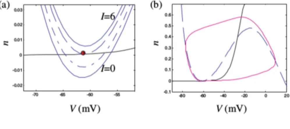
system (4.9)–(4.10) is known as planar, as its phase space is the two-dimensional plane spanned by V (the abscissa) and n (the ordinate). To understand the dynam-ics we calculate the nullclines for the dynamical variables V and n. In Fig. 4.5 is

FIGURE4.5: (a) Representative sub- (green) and supra-threshold or-bits (red) and (b)their temporal evolution. The nullclines are drawn

with the parameters value found in [19].

shown representative orbits of this system. Three “subthreshold” (green) and three “suprathreshold” (red) orbits are shown. In the latter case, the neuron depolarizes before returning to its resting state. It should be noted that this threshold depends not only on the initial membrane potential V but also the initial K+membrane con-ductance. The separatrix between sub- and supra-threshold is constituted by the inset of the saddle point (not shown). Whether the initial condition is sub- or supra-threshold, this system only has a single steady state solution in the current parameter regime. Hence, after at most one depolarization, it enters a quiescent state. There-after a discrete synaptic input, such as due to an excitatory post-synaptic potential

Computational study of resting state network dynamics