Wind pattern analysis applied Tokyo 2020 Olympic Game

(1)

Alma Mater Studiorum · Università di Bologna

SCUOLA DI INGEGNERIA E ARCHITETTURA

DIPARTIMENTO INFORMATICA - SCIENZA E INGEGNERIA Corso di Laurea Magistrale in Ingegneria Informatica

TESI DI LAUREA in

Intelligent Systems M

WIND PATTERN ANALYSIS

APPLIED TO TOKYO 2020

OLYMPIC GAME

Relatore:

Prof.ssa Michela Milano

Prof.ssa Alicia Ageno

Presentata da:

Fabio Di Francesco

Sessione I

(2)

(3)

Acknowledgements

I would like to thank Professor Ageno for the great help in the work of this thesis, as well as TriM team, that provided knowledge and suggestions about this field that was new to me, and also Meteocat that was always available to give information and explanation on the data used that allowed to develop the implementation of this project.

(4)

(5)

Abstract

The following master thesis is the product of the work carried out during the Erasmus exchange of the year 2017-2018 that involved the author, exchange student from the University of Bologna, the Universitat Politècnica de Catalunya , TriM, an italian company with a strong knowledge of weather data and forecasting, and Meteocat, the public meteorological company of Catalonia in a collaboration aimed to find new methodologies for the processing of meteorological data.

The reason that motivated this work is dictated by the increasing amount of weather data available today, that necessarily drives the weather forecasting in a more automated procedure that reduces the time needed to generate a forecast and the intervention of a human, in the figure of a meteorologist, in the analysis of the data. This allows to process more data and thus having predictions that take advantages of the usage of many information that could result in improved forecasting.

The development in the field of machine learning allows today to treat a vast amount of information in an automatic way, leaving the analysis process to the machines, freeing the user of this time-consuming task. And unsupervised learning is the branch that can process data that are not labelled nor preprocessed, speeding up the data mining.

The goal of this thesis is to apply unsupervised learning techniques to this scope, taking inspiration from the available literature that experimented in this field and combining different solutions into a new technique that aims to reduce the human decision in the process of the recognition of wind patterns and improve the automation of the whole process.

(6)

(7)

3.6.1 Manual clustering . . . 32 3.6.2 Automatic clustering . . . 33 3.6.2.1 Quality measures . . . 34 3.7 Clustering comparison . . . 36 3.8 Classification . . . 38 4 The implementation 39 4.1 First attempts . . . 39 4.2 Data Loading . . . 40 4.3 Normalisation . . . 42 4.4 Hierarchical Clustering . . . 43 4.4.1 Automatic clustering . . . 43 4.4.2 Manual clustering . . . 45 4.5 K-means . . . 47 4.6 Results report . . . 49 4.7 Classification . . . 51 5 Results Analysis 53 5.1 Meteorological analysis of clustering results . . . 53

5.1.1 Automatic clustering . . . 55

5.1.2 Manual clustering . . . 57

5.1.3 Automatic clustering revisited . . . 58

5.2 Classification results . . . 60

6 Conclusion 65 6.1 Future Work . . . 66

References 71 Appendix A Automatic clustering results 75 A.1 Automatic clustering infos . . . 75

A.2 K-means infos . . . 76

(9)

Table of contents ix

Appendix B Manual clustering results 91

B.1 Manual clustering infos . . . 91

B.2 K-means infos . . . 91

B.3 Manual clustering results, k = 17 . . . 92

B.3.1 Threshold . . . 92

B.3.2 Comparison with automatic clustering . . . 107

B.3.3 Comparison with manual clustering k = 10 . . . 107

B.4 Manual clustering results, k = 10 . . . 109

B.4.1 Threshold . . . 109

B.4.2 Comparison with automatic clustering . . . 119

(10)

(11)

List of figures

1.1 Representation of the components of the solution . . . 4

2.1 Vector representation of the wind flow . . . 8

2.2 The area covered by AROME . . . 11

2.3 Screenshot from PanoplyJ . . . 15

2.4 Georeferenced Plot . . . 16

2.5 Representation of the values stored in the NetCDF file . . . 17

2.6 The 16 points chosen for WRF . . . 18

2.7 The 16 points chosen for AROME . . . 19

3.1 Examples of dendrograms . . . 25

4.1 Initial screen of the application. . . 40

4.2 Section of data normalisation. . . 42

4.3 Section of hierarchical clustering. . . 43

4.4 Section of automatic hierarchical clustering. . . 43

4.5 Section of manual hierarchical clustering. . . 46

4.6 Section of k-means. . . 47

(12)

(13)

List of tables

2.1 Example of WRF file . . . 10

3.1 Types of linkage . . . 26

3.2 Quality measures . . . 36

5.1 Clusters division by direction . . . 57

5.2 Clusters matching . . . 61

5.4 Clusters similarity . . . 62

5.4 Clusters similarity . . . 63

A.1 Clusters information . . . 77

A.4 Ranges of TEMPERATURE (in °C): . . . 80

A.5 Ranges of HUMIDITY (in %): . . . 81

A.6 Ranges of PRECIPITATION (in Kg/mˆ2): . . . 82

A.7 Ranges of PRESSURE (in Pa): . . . 83

A.8 Wind speed ranges (in m/s) . . . 84

A.9 Wind direction ranges . . . 85

A.10 Wind direction ranges . . . 86

A.11 Wind direction wider ranges . . . 87

A.12 Transition matrix . . . 88

B.1 Clusters information . . . 94

B.4 Ranges of TEMPERATURE (in °C): . . . 97

B.5 Ranges of HUMIDITY (in %): . . . 98

(14)

xiv List of tables

B.7 Ranges of PRESSURE (in Pa): . . . 100

B.8 Wind speed ranges (in m/s) . . . 101

B.9 Wind direction ranges . . . 102

B.10 Wind direction wider ranges . . . 103

B.12 Transition matrix . . . 105 B.13 Clusters matching . . . 107 B.14 Clusters matching . . . 107 B.15 Clusters information . . . 111 B.16 Clusters information . . . 111 B.17 Clusters information . . . 112

B.18 Ranges of TEMPERATURE (in °C): . . . 112

B.19 Ranges of HUMIDITY (in %): . . . 113

B.20 Ranges of PRECIPITATION (in Kg/mˆ2): . . . 113

B.21 Ranges of PRESSURE (in Pa): . . . 114

B.22 Wind speed ranges (in m/s) . . . 114

B.26 Transition matrix . . . 117

B.27 Clusters matching . . . 119

(15)

Nomenclature

Acronyms / Abbreviations

AROME Applications of Research to Operations at MEsoscale

E East ENE East-North-East ESE East-South-East NE North-East N North NNE North-North-East NNW North-North-West NW North-West

NWP Numerical Weather Prediction SE South-East S South SSE South-South-East SSW South-South-West SW South-West WNW West-North-West

(16)

xvi Nomenclature

WSW West-South-West

(17)

Chapter 1 Introduction

1.1 Meteorology

Meteorology is the science that studies the atmosphere and the events connected to it. One of the main focus of meteorology is to produce weather forecasting, that is the application of the principles of meteorology in order to predict the phenomena that will happen in a given place and time. Various data are collected from instruments and sensors, and their changes over the time are studied to understand the meteorological phenomenon that is taking place and to construct models to be used for the prediction. This process requires the interpretation of a human, to choose the right model for the prediction and to interpret the results.

Weather forecasting is not only delivered to the general public, but there are some specific sectors that needs a forecast to operate and grant safety. For example, air traffic needs accurate weather forecasting to plan airplane routes in order to avoid thunderstorm or prevent icing of the wings. Furthermore, forecasting is helpful to prevent and control wildfires.

Lastly, an important application of weather forecasting is for navigation in waterways as weather can strongly influence the safety of the transit due to the wind, waves and tides. So, in this case, the wind plays a fundamental role, along with other weather parameters.

1.2 The scope of the thesis

The scope of the thesis focuses on marine weather forecasting, particularly in the study of wind patterns. The present master thesis is developed in the framework of the

(18)

2 Introduction

Tokyo2020 Olympic Games Weather Project, led by TriM company and funded by the Austrian Sailing Federation and by Croatia and Cyprus Laser Olympic classes. Sailing strategy and performance are strongly related to environmental parameters such as weather, oceanic current and geographical data. A thorough prediction of the conditions expected during a sailing race is a piece of valuable information for a sailor, as it completely conditions his/her tactics during the race. Therefore, within the Tokyo 2020 Weather Project a big amount of data are produced both by collecting data on the sea and by running numerical weather prediction models. All these data are stored into a cloud database.

1.3 The motivation

The increasing number of meteorological data available from weather models together with recent developments of technology represent a significant opportunity for the identification of repeatable weather patterns that can support actors working within complex environmental systems. Nevertheless, at the moment, the identification of weather patterns still involves a subjective interpretation from a meteorologist who is linking data coming from numerical weather prediction models, numerical data collected on the field and qualitative signs observed in different weather conditions. This process requires a significant human effort, resulting in a slower analysis of a limited number of data. Moreover, if the area of interest changes, all the manual process should start from the beginning. Automatizing this process would mean spending less time in generating predictions, which would permit the analysis of a wider range of meteorological data and would provide procedures that can be reused for different places. Consequently, better forecasting could be produced as it would take into account as many parameters as possible and it might be more easily quickly updated.

1.4 Objectives

The aim of this work is to find a manner to analyse automatically this data using machine learning, which is a technique that allows a computer to learn from data without being specifically programmed. The goal is to give added value to traditional classification schemes for wind patterns, based on meteorological experience and manual analysis of synoptic weather charts. A methodology based on clustering able to automatically induce wind patterns based on collected data, as well as the characteristic features of these patterns and their evolution through the day, will be developed and

(19)

1.4 Objectives 3

tested. The different automatic clustering that will be tested could also be able to describe different behaviours of the wind in different sailing areas, within the same wind pattern. All these would allow:

• A detailed analysis to determine the representativeness of the wind fields encoun-tered during training and racing period, their frequency of occurrence, timing, rate of evolution, and transition probabilities.

• Consequently, a more thorough prediction of the conditions expected before a sailing race, which is as mentioned a highly valuable information for the sailor. The system developed will be fed with meteorological data and apply machine learning in the form of clustering analysis that consists of grouping together elements that have similarities, to find a common pattern of winds to be used to plan the strategy in boat racing. Machine learning indeed fits very well this scope as it requires as many data as possible, and the measurements collected from sensors are many. What will be explained throughout this document is the technique used to find these patterns.

There are multiple applications of different techniques of clustering for finding different kinds of weather patterns. For example, Aran et al. [1] apply PCA analysis in combination with k-means clustering plus Discriminant Analysis to detect weather patterns associated with strong wind events in Catalonia. In this case, in order to compute this classification, the chosen algorithms that will be employed are hierar-chical clustering and k-means. In the literature, there are already attempts to take advantage of these two algorithms to analyse winds. In particular the works of Kaufmann and Whiteman [2] and Kaufmann and Weber [3] are two studies where this methodology was applied. In [2] they analyzed wind pattern in the Gran Canyon using data coming from meteorological stations. This paper was indeed the main reference as they proposed solution very suitable for the scope of this work. In spite of that, it is important to emphasise that the wind patterns object of this work aim to be far more specific than theirs, since a race in Olympic sailing takes place in a very small area (around 2-3 nautical miles), and the forecast needed must be far more accurate than a conventional weather forecast: the solution is aiming for the prediction of variations in direction of the wind of 5-10 degrees and variations of 2-5 knots in its intensity during the span of 3-6 hours that the races may last. Furthermore, their work was more focused on the meteorological aspect, so this research wanted to go deeper in the machine learning aspect, trying to improve their work using a methodology studied by Surdeanu et al. [4], that similarly to Kaufmann and Whiteman used clustering to group documents, but improving the automation of the algorithm, as the choice of the right

(20)

4 Introduction

number of clusters after the hierarchical clustering was taken by the algorithm. These two approaches will be combined together: finding automatically the optimal value for the number of clusters in hierarchical clustering and apply it in k-means. It should be noted that, although the ultimate goal is to apply this automatic methodology to the actual collected data, at the moment of implementing this work these data were not available yet since the collection of data in Tokyo started in August 2018 (and will last until 2020). Therefore, our methodology will only be applied to the output from the numerical weather prediction models. High resolution weather models provide wind forecasts for specific areas and specific ranges of time. Although of course, it can always be the case that what is forecasted is not what actually happens in the end, it can be a good approximation. The idea is to develop and test the methodology, and in case the results are promising, it will be easy to extrapolate it to whatever geographical area and whatever type of input data, either collected or generated from the weather models.

The project was developed to work independently by the site chosen, and, given that meteorological data of the sites of Tokyo where the races will take place are not yet available, measurements of Barcelona area were used to study, train and check the program.

The program was realized in Python chosen firstly for a discreet number of library dedicated to machine learning. These however revealed not to be suitable for the context treated in this work, so the algorithm was written by scratch while using different libraries for the computational part and the processing of the data.

1.5 Structure of the solution

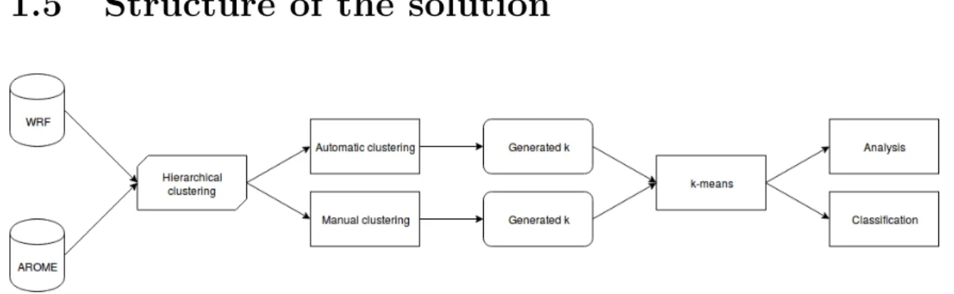
Fig. 1.1 Representation of the components of the solution

In figure 1.1 it’s possible to see how the solution is structured: the available data comes from two different sources of meteorological data, AROME and WRF. This two

(21)

1.6 Next chapters 5

sources came with different file representation but both covered the area of Barcelona and they were analyzed in the same way.

The data was firstly processed by hierarchical clustering, in particular in the two different approaches that were mentioned before: Automatic clustering corresponds to the work of Surdeanu et al. [4] while the Manual Clustering is a plain execution of a hierarchical clustering, as done in Kaufmann and Whiteman [2]. This two different executions both produce k, the number of clusters to be used in k-means.

Once the classifications are complete, it produces a series of statistics and graphs that are analyzed to check if the resulting classification was able to group wind patterns characterized by similar measurements values and to compare the two different approaches.

1.6 Next chapters

In the following chapter 2 the datasets used will be examined, as well as the type of files used to represent them. Next in chapter 3 the theoretical notion of clustering regarding the algorithms used will be explained and, after that, in chapter 4 how they were implemented in this work. Subsequently, chapter 5 is dedicated to the analysis of the results obtained from the data and the algorithms. Lastly, the conclusion and the thoughts for further work in chapter 6 close this thesis.

(22)

(23)

Chapter 2 The meteorological data

2.1 Data collection

The first step in the process that leads to weather forecasting is the data collection. This is usually done with satellites or weather stations equipped with different instruments, like barometers, thermometers, anemometers and more. These can be stations on the ground, or, as this will be the scope of this work, dedicated buoys to measure weather data in the sea.

2.2 Types of data

As we said the meteorological stations are furnished with many instruments that check various air parameters. In this work different types of parameters, know by the general public, are used:

• temperature • humidity • pressure

• total precipitation

In addition to these, there are two parameters that are the most important and the ones used in the algorithm calculations, that are related to the wind. They are the wind u and v components that are the mathematical representation of the wind flow as a vector.

(24)

8 The meteorological data

The wind has a speed and a direction. These two elements can be completely defined by a vector.

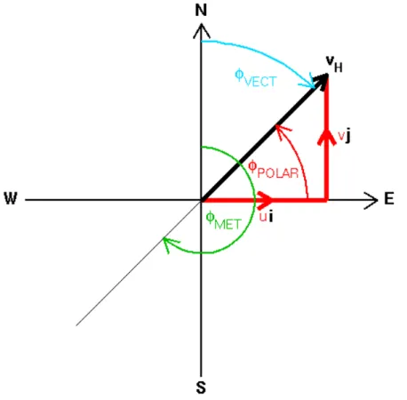
Fig. 2.1 Vector representation of the wind flow

From the figure 2.1 [5] is possible to see the vector defined by a wind flow vH. The components u and v (also called eastward direction and northward direction) are the projections of the vector on the axis. The representation of the direction, however, is not simply the angle ϕpolar generated by the vector with the x axis (corresponding to

E in the figure 2.1). There are two conventions to represent the direction: one is the wind vector azimuth, that is the direction where the wind is blowing, corresponding to

the angle ϕV ECT in the figure. The other is the meteorological wind direction, i.e the direction from which the wind is blowing, represented by the green arch ϕM ET. It is important to keep in mind this representation in the section of calculation, otherwise, this could lead to a wrong interpretation of the meteorological data.

In the rest of this document, the direction will be always considered as meteorological

(25)

2.3 Data sources 9

2.3 Data sources

2.3.1 Numerical Weather Prediction

Numerical Weather Prediction, or NWP, [6, 7] is a method of weather forecasting that employs mathematical models of the atmosphere that use current weather conditions to elaborate forecasting. An NWP is calculated with the help of a computer and there are many distinct models available that differ based on the atmospheric processes they are applied to or the part of the world that they analyze. The current weather observations are the input of numerical computer models that calculate outputs of many meteorological parameters, like temperature, pressure and many more, thanks to a process called data assimilation. So both the meteorological measurements and the numerical computer models have great importance in the forecasting.

The numerical models used consist in equations of fluid dynamics and thermody-namics that describe the atmosphere behaviour and predict it. Such equations are complex to solve and require to be simulated on super computers. This is a reason because meteorological forecast can predict weather up to six days, and also because the equations are nonlinear partial differential that cannot be solved exactly but the results obtained are approximate solutions, and the error grows with time.

The data that has been used for this work comes from two different weather models: WRF and AROME.

2.3.1.1 WRF

The Weather Research and Forecasting (WRF) [8] Model is a mesoscale numerical weather prediction system developed starting in the latter part of the 1990s, designed for atmospheric research and forecasting application. It was developed in the US by many research entities and universities and today is maintained by the National Center for Atmospheric Research (NCAR). It is composed of two dynamical cores, a data assimilation core and a parallel and extensible software architecture. It can produce simulations using actual atmospheric conditions or idealized conditions. WRF can count on a large developers and users community and it is widely used for meteorological bulletin as well by researchers and laboratories.

This is a high resolution model that serves applications across scales from tens of meters to kilometers and is not freely available to the public. For this reason, this meteorological data was provided by Meteocat, the meteorological service of Catalonia. In this project they collaborated providing the data and the know-how on how to deal with different kinds of files. From this model, they furnished the files with

(26)

the six weather parameters mentioned earlier needed in this project, in csv (comma separated values) files.

The data is contained in csv files that cover all month of March and April 2018. Each file represented a precise time and date of the period and contained the value of one measurement over different locations of the area of Catalonia. As said in 2.2 the types of data used are 6. That means that for every timestamp there were 6 different files each containing one measurement.

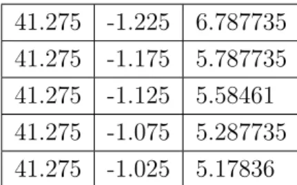
Table 2.1 Example of WRF file 41.275 -1.225 6.787735 41.275 -1.175 5.787735 41.275 -1.125 5.58461 41.275 -1.075 5.287735 41.275 -1.025 5.17836

The table 2.1 shows an extract of a csv file: the first column is the latitude, the second is the longitude and the last one is the measurement. Using this type of files was particularly easy: first of all, it is a common and spread text file format where values are separated by commas, or other special characters, stored in tables. It is also easy to read with just a spreadsheet program, like Microsoft Excel. These files are small in size and each of them was less than 30 KB, and, even if each of the six parameters was saved in a single file, the whole data set is, yes composed by more than 8000 files, but still occupied a total space in local memory of 240 MB, a huge difference in what will be seen with the AROME dataset. Lastly operating with csv files in Python is straightforward: the function genfromtxt from numpy, a powerful library of Python that allows to manipulate data and mathematical functions, read the all file row by row, and save it in an array.

2.3.1.2 AROME

AROME, Applications of Research to Operations at MEsoscale, [9] is a small scale numerical weather prediction model, maintained by Meteo-France, designed for short term forecasting, in particular for severe atmospheric phenomenons, like storms in the Mediterranean. It covers all France territory and waters and most of Spain.

(27)

2.3 Data sources 11

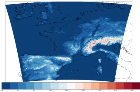
Fig. 2.2 The area covered by AROME

AROME collects data from radar networks to produce hourly based models with a high resolution. It is used to produce five days weather predictions but it has also proven to be useful with severe precipitations.

This data was provided instead by TriM that was the main partner in this project that along data contributed with knowledge and collaborated with Meteocat too.

The original data were saved in GeoTIFF files, one for each parameter. TIFF, Tagged Image File Format, is a tag-based file format designed to store and share raster images. GeoTIFF is an extension compliant with TIFF specifications used to store georeferenced information thanks to certain TIFF tags.

It was planned to merge all the measurements of one day in a single file and, as a result of the meetings and advice from Meteocat, there are two files suitable for this:

GRIB and netCDF.

GRIB files One choice to store the meteorologic data was GRIB (GRIdded Binary or General Regularly-distributed Information in Binary form) files [10, 11]. This particular file format is commonly used in meteorology to store weather data. Created by the World Meteorological Organization (WMO) it is a collection of records of data, in the form of tables, thought to transfer volumes of gridded data efficiently. Data packed in a GRIB are more compact than a text-oriented file, which means smaller files to store large amounts of meteorological data. There are two versions of GRIB currently used, GRIB1 and GRIB2. They differ for additions of new parameters or

(28)

more precise definitions of the existing ones. A record of a GRIB file represents a parameter described by gridded values or coefficients. In this case, the parameters represent the u and v values, temperature, humidity, pressure and total precipitations.

To operate with this kind of files there are different libraries and programs. The most used is wgrib, available as a bash command in Linux. The usage is quite simple, it allows to decode GRIB files and read their contents or convert them into other files. Despite its spread, GRIB files present some disadvantages that prevented to be used in this project. As said before, there are two main versions of GRIB and to read GRIB2 is necessary to use wgrib2. It requires many dependencies from other libraries to be installed therefore it was hard to configure everything correctly. Furthermore the parameters can be set differently as well as the grid of coordinates used. Lastly the output decoded from a GRIB file using wgrib is not easy to interpret. For example the output from a simple wgrib command of a wind measurement file is the following:

$ w g r i b Lyon−B a l e a r e s . grb

1 : 0 : d =18092018:UGRD: kpds5 =33: kpds6 =105: kpds7 =10:TR=0: P1=6:P2=0:TimeU=1:10 m above gnd : 6 hr f c s t : NAve=0 2 : 5 1 1 8 6 : d =18092018:VGRD: kpds5 =34: kpds6 =105: kpds7 =10:TR=0:

P1=6:P2=0:TimeU=1:10 m above gnd : 6 hr f c s t : NAve=0 3 : 1 0 2 3 7 2 : d =18092018:UGRD: kpds5 =33: kpds6 =105: kpds7 =10:TR=0:

P1=9:P2=0:TimeU=1:10 m above gnd : 9 hr f c s t : NAve=0 4 : 1 5 3 5 5 8 : d =18092018:VGRD: kpds5 =34: kpds6 =105: kpds7 =10:TR=0:

P1=9:P2=0:TimeU=1:10 m above gnd : 9 hr f c s t : NAve=0

This an extract of the command result. Firstly it can be noted that it is not very easy to understand. It includes information on the data like the byte offset, that is not vital to understand the content, while other data are stored in the values kpds: kpds5 with value 33 states that it is a u-component of wind; kpds6=105 that it is measured at a certain value above the ground and lastly kpsd7=10 that the measurement took place every 3 hours. However, all this information present in kpsd values can be understood only by checking the tables in the documentation of grib files that explain what each value represents. This is clearly not very immediate to understand and requires time to research the meaning of a value. To overcome this problem, it was agreed that all AROME files used in the project should have been converted into NetCDF files. netCDF netCDF (Network Common Data Form) [12] is another format to store array-oriented scientific data in a portable and self-describing file, that means that this kind of file can be accessed on different platforms, regardlessly how they represent

(29)

2.3 Data sources 13

integers, floats and characters, and also that the dataset includes a description of the data that is stored, like the units of measurement.

This type of file is developed and maintained by Unidata that is part of the University Corporation for Atmospheric Research (UCAR), indeed there are many tools provided by Unidata to work with geoscience data. As said the data are in form of arrays and this includes arrays of dimension n > 1, and the data used in this project are an array of dimension 3, latitude, longitude and time. This can be seen as a 3-D matrix composed by 24, as the daily hour, 2-D matrices with the dimensions of the area covered by the meteorological data, each element of the matrix containing the measurement of the parameter.

This file has evolved through the years and there are different versions released over the years. Until version 3.6.0 the versions of netCDF employed one binary format. These are referred to as the classical format. After 3.6.0 a 64-bit offset format was adopted allowing to use file bigger than 2 GiB. The last version 4.0.0, called netCDF-4, started using another binary format HDF5, which is a spread data model for storing and managing data, capable of supporting a wide variety of datatypes. It is designed to be flexible and efficient thus is portable and extensible.

The new versions allowed the netCDF file to store a larger amount of data with the 64-bit offset update and with the netCDF-4 format it was possible to use a more complex representation of data, like groups, nested trees and variable length array.

Despite the improvements of the newer versions, the classic format is the one that grants the maximum compatibility as the usage of later versions requires the interfaces and programs to be updated. So in this project, the format for the netCDF files is classic format.

This kind of file can be read easily via a Unix command, ncdump. In the following example, we can see an extract of the structure of the variables of one AROME file.

$ ncdump −h AROME_2018−04−06. nc d i m e n s i o n s : tim e = UNLIMITED ; // ( 4 8 c u r r e n t l y ) l a t = 561 ; l o n = 590 ; v a r i a b l e s : d o u b l e Band1 ( time , l a t , l o n ) ;

Band1 : long_name = " eastward_wind " ;

Band1 : _ F i l l V a l u e = 9 . 9 6 9 2 0 9 9 6 8 3 8 6 8 7 e+36 ; Band1 : grid_mapping = " c r s " ;

(30)

d o u b l e Band2 ( time , l a t , l o n ) ;

Band2 : long_name = " northward_wind " ;

Band2 : _ F i l l V a l u e = 9 . 9 6 9 2 0 9 9 6 8 3 8 6 8 7 e+36 ;

A classic format netCDF is composed of two parts, the header and the data. The

-h argument of ncdump shows the header. This describes the type of content and how

it is represented. It is possible to see that the dimensions that describe the variables are 3, time, latitude and longitude. This means that data vary by these 3 dimensions. Time, in particular, is defined as unlimited that is used for dimensions that can be extended, in cases when the total length is not known or it is necessary to add more data. On the other hand, latitude and longitude are well defined because a specific area is covered.

Speaking of the variables, two of the total 6 are present in the extract. They are a 3 dimensions array, represented by double values defined by the three dimensions and are respectively the u and v component. It is possible to specify a default value when some are missing, a name for the variable and the mapping of the grid used and the real coordinates.

Using this kind of file within Python was easy, it was just necessary to install a module, simply called netCDF4 that uses a class called Dataset. Accessing the data was relatively simple too, accessed as a 4 dimensions array, one dimension for the variable name (i.e. Band1, Band2, etc.) and 3 for the dimensions time, latitude and longitude.

Using such files revealed easy and handier than GRIB files, nevertheless, this type of format had a con, that is its size. The files used to store AROME data were on average 700 MB for a total of 40 GB for the complete dataset, and this affected the program performances on the loading of the data, a significant difference with the csv file of WRF.

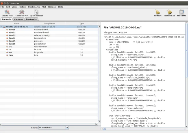
A useful program used during this work to inspect and check NetCDF file was PanoplyJ, developed by NASA. Thanks to this program it was easy to check the types of variables stored in the file and how they were structured.

(31)

2.3 Data sources 15

Fig. 2.3 Screenshot from PanoplyJ

From the screenshot of PanoplyJ in figure 2.3 we can understand better the composition of these files. On the right, there is a pane with the same information given by ncdump, regarding the dimensions and variables. On the left pane, all the variables and dimensions are single elements in a table, with additional information. Long names and the type of data are clearly expressed; it is interesting to note that the different variables Bands are Geo2D type. Indeed they are a collection of 2D matrices georeferenced data, in this case 48.

In PanoplyJ, is also possible to plot them on a map and have a visual representation of the values.

(32)

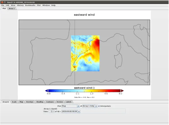
Fig. 2.4 Georeferenced Plot

(33)

2.3 Data sources 17

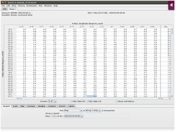
Fig. 2.5 Representation of the values stored in the NetCDF file

Every cell is the value of the measurement in a certain place given by the coordinates in the row and column header. The whole day is represented by 24 of these tables (even 48 as it is forecast also the following day) that can be selected in the lower part

of the window of figure 2.5. This table is exactly what will be loaded in Python. During the work on the project however, it surfaced that some values of the temperature of the days of May were wrong, indeed they had values of more than 10000. Checking the files with Panoply and talking with TriM revealed that there had been a mismatch during the conversion into netCDF. Firstly a workaround was used to exclude these wrong values in the code of the program, then the files were fixed, as those mismatched values referred instead to pressure. This has affected marginally the initial results during tests because, as said before, the main values used by the algorithm are u and v. Anyway in the final results, this mistake was corrected.

Choosing netCDF as the format to operate with revealed the best choice, weighting the compromises between the ease of use and the performance.

(34)

2.3.2 Area of measurements

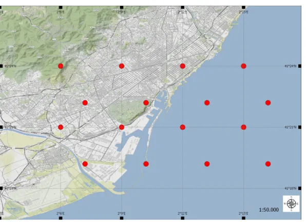
This calculation is aimed for the area of Tokyo that is where the sailboat races will take place. However measurements from Japan are not yet available, so to test the program it was chosen the bay of Barcelona, due to both the availability of high resolution data and the knowledge of the area from the supervisor of this thesis and TriM. This knowledge will be very valuable when analyzing the usefulness and coherence of the results obtained.

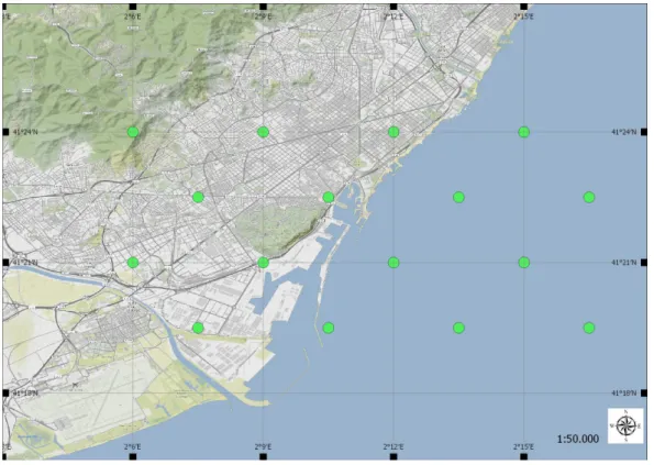
As in Kaufmann and Whiteman [2] there were weather stations measuring wind data, in this project 16 coordinates of the two weather model were taken as to simulate measuring station. These comprehend both points on the land and in the sea.

Fig. 2.6 The 16 points chosen for WRF

As it is possible to see in figure 2.6 half of the points are on the land while the other in the sea. In this way, it was possible to test the program with winds that characterise different locations.

The points chosen for AROME are quite similar but they differ slightly just because the WRF has a higher resolution, although they can be considered corresponding.

(35)

2.3 Data sources 19

(36)

(37)

Chapter 3 Clustering

3.1 Machine Learning

There are many definitions of machine learning. The most famous is the one gave by Arthur Samuel, a pioneer in machine learning in 1959: ′′Machine learning is the field of study that gives computers the ability to learn without being specifically programmed”.

There is also another definition, more formal, gave by Tom Mitchell: "a computer program is said to learn from experience E with respect to some task T and some performance measure P, if its performance on T, as measured by P, improves with experience E" [13].

In some way the aim is to imitate how the human brain learns, using statistical techniques and algorithms.

There are many and different learning algorithms, but they can be grouped into two main categories depending on how the algorithm learns: supervised and unsu-pervised learning.

In supervised learning, given a dataset, it is already known what is the correct output, so every measurement has a corresponding response. It is like teaching a computer what is right and what is wrong, giving it examples on how it should answer with specific inputs and learn the rule that maps inputs with correct outputs. Examples of supervised learning are regression, where input is mapped on a continuous output, and classification, where the predicted outputs are discrete, that means starting from inputs find the corresponding outputs in a series of classes or categories [14].

On the other hand, in unsupervised learning the dataset has no correct output, so it is not possible to teach the computer how a correct answer should be, it has to learn it by itself. In this case, it is harder to analyse the results of a learning algorithm since the correctness of the output is unknown to the programmer too and the goal

(38)

22 Clustering

is to find patterns in the data. Nevertheless, the advantage of unsupervised learning algorithms is that it is easier to find unlabelled data rather than labelled data, that requires human intervention [15]. Examples of unsupervised algorithm are clustering,

dimensionality reduction and neural networks.

Dimensionality reduction consists of reducing the dimension of the data that need to

be analysed to optimised computing time and costs. It assumes that data is redundant and that it can be represented with only a fraction of it [16] [17]. There are two popular algorithms to reduce dimensionality:

• Principal Component Analysis (PCA), that produces a low-dimensionality of a dataset, finding a linear combination that gives the maximum variance;

• Singular-Value Decomposition (SVD), that allows to represent data as a product of 3 smaller matrices.

Deep learning is a relatively new approach, based on the use of neural networks, that

tries to imitates how brain cells work, decomposing the problem in smaller tasks adopting elements called perceptrons that calculate output using functions and weights, composed in single or multiple layers. [18, 19]

Lastly clustering, that is the topic of this work, will be examined more in detail.

3.2 Fundamentals of clustering

Clustering is a machine learning technique where the aim is to find clusters, or groups, in a dataset. As said it is part of unsupervised learning, which means the input data is not labelled by a supervisor nor there is any indication of what defines a good value or a bad value.

Clustering the observations of a dataset means partition them in groups of objects that are similar to each other, while clustering objects that are different in other groups.

′′_{Similar”, however, is a generic concept and depends on the domain of application.}

[14]

As an example, it can be taken a series of clinical data from cancer patients. The samples of the dataset are expected to be heterogeneous, depending on the patient data. However certain aspects or subgroups of them could be similar between some, defining a certain type of cancer or other common characteristics. Clustering these data could help to find this common subgroups without having to classify them previously.

The field of application of this kind of method are numerous, thanks to the fact that data does not need to be preprocessed. As said they can be used with clinical

(39)

3.2 Fundamentals of clustering 23

data, but also in marketing to group clients that have common characteristics who can be the target of an effective advertising campaign or to drive them to the most suitable purchase.

Also they can cluster documents, for example, newspaper articles, dividing them in bags of words, and can be categorized by type (sport, economics, politics, etc.)

There are many clustering algorithms: hierarchical clustering and k-means are among the most spread and are the ones adopted in this project, but there are other important clustering algorithms such as DBSCAN and Expectation-Maximization, which have been discarded because they do not apply to our specific methodology, as described in section 1.5. However, they will be briefly mentioned as well due to their importance in the clustering group.

DBSCAN [20, 21] is a density-based cluster algorithm that is a class of clustering

where clusters are defined as an area of higher density compared to the rest of the data, while sparse objects are considered noise. With this kind of clustering is possible to discover clusters of arbitrary shape. DBSCAN, in particular, is based on the concept of density-reachability that defines a cluster as a maximal set of density-connected object. Objects are divided into three categories:

• core, that are the objects which have a minimum number, defined as a parameter, of other objects within a distance threshold;

• border objects have fewer elements than the minimum number in their neighbour, but are in the neighbour of a core object;

• outlier or noise object, that are neither core nor border objects. So a cluster is composed of core and border points.

DBSCAN pros are that it is able to ignore noise and handle clusters of different shapes and sizes. However, it needs an area where the density is lower to recognise the border of a cluster.

The distribution of objects can be also hypothesised to be a mixture of distributions where every group is generated by a single distribution but all the groups together appear as generated by a unique one.

The goal of Expectation-Maximisation (EM ) [4, 22–24] is to find the original distributions. To simplify the process they are considered all the same type, usually Gaussian. EM tries to find the parameters of the distributions calculating the log-likelihood, a simplification of the maximum likelihood estimation. EM executes iteratively the two steps Expectation and Maximisation: in the expectation phase,

(40)

24 Clustering

the expected value of the log-likelihood is calculated, while in the maximisation phase the expected value previously calculated is maximised to determine the distribution parameters. The process is repeated until convergence, that assured since the algorithm maximises the likelihood at every step.

3.3 Hierarchical Clustering

Hierarchical Clustering [14, 25] is one type of clustering that uses a distance function to establish if two objects are similar and thus be in the same cluster. Usually, Euclidean distance is used when attributes have the same scale

d(x, y) = n v u u t n X i=1 (xi− yi)2 (3.1)

There are also other distance functions, like correlated-base distance. It considers two observations similar if their features are correlated, even if they are far with Euclidean distance. For example, customers that buy few items can be clustered together, but maybe their shopping preferences might be very different; correlation-base distance would pair people with similar preferences independently of the number of purchases. Hierarchical clustering can be bottom-up or agglomerative, i.e. it starts with N clusters, each containing only one element and each step of the clustering consists in merging the two most similar until only one cluster is obtained. The opposite is the

top-down or divisive clustering that starts from a unique group and divides it until

every observation is in one group. This work will use the agglomerative version, which is also the most common one, starting from a group for every wind observation.

The result of Hierarchical clustering is a dendrogram, a tree-based representation of the observations. The leaves represent all the observation and the tree shows how they are merged.

(41)

3.3 Hierarchical Clustering 25

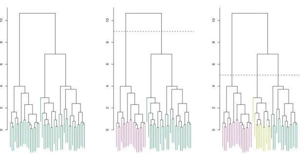
Fig. 3.1 Examples of dendrograms

Figure 3.1[14] shows some examples of dendrograms. From the y axis we can see how distant two elements are: the shorter vertical line that connects two observations is, the more similar the observations are. And moving up the tree gives an indication of the order of the merging because the two closest elements are the ones chosen to be joined, so the first horizontal line that connects two elements is the first cluster to be created.

The dashed lines in the second and third dendrograms is the height at which the dendrograms are cut, respectively 9 and 5. The number of intersections with the vertical lines represents the number of clusters that will be formed. Cutting the dendrogram at a height of 9 gives two clusters that contain respectively the elements in red and green. Instead, the height of 5 gives three final clusters. The height of the cut controls the number of clusters obtained.

The downside of this technique is the choice of the height, so the choice of the number of clusters. This is usually done by observing the clusters and picking an arbitrary height. Clearly, this is not the best solution, as it could require more attempts or either is not easy to understand for complex data if a cluster has effectively similar observations.

3.3.1 The algorithm

The algorithm of this method, illustrated in Algorithm 1, is really easy. It first needs a dissimilarity measure to sort the observations. Usually, for simple elements, Euclidean

(42)

26 Clustering

distance is a common choice. The algorithm works iteratively, starting from the leaves of the dendrogram where each of the observation has its own cluster. At each step the two most similar groups are merged, so after there are n − 1 cluster. At the next step, they become n − 2 and so on until all of them are grouped in a unique cluster.

During the execution the algorithm merges the two closest clusters it finds. This concept is straightforward when two single elements are considered, but for clusters with more than one element is necessary to choose a point that will be used to calculate the distance. So to extend the notion of distance to groups of observations, the linkage function was introduced, that calculates the distance between arbitrary subsets of the dataset. The most common types are single, complete, average and centroid linkage.

Table 3.1 Types of linkage Linkage Description

Single linkage

Computes all the possible distances between the elements of cluster A and cluster B and chooses the shortest distance of all.

Complete Linkage

Computes all the possible distances between the elements of cluster A and cluster B and chooses the largest distance.

Average Linkage

Computes all the possible distances between the elements of cluster A and cluster B and calculates the average of them.

Centroid Linkage The distance is the point distance between the means, i.e. the centroids, of cluster A and B.

Mathematically they can be expressed as follows

LSingle(A, B) = min

x∈A,y∈Bd(x, y) (3.2)

LComplete(A, B) = max

x∈A,y∈Bd(x, y) (3.3)

LAverage(A, B) =

P

x∈A,y∈Bd(x, y)

(43)

3.4 K-means 27 LCentroid(A, B) = d P x∈Ax |A| , P y∈By |B| ! (3.5)

Complete and average linkage are preferred over single linkage as they produce a more balanced dendrogram. Moreover, average and centroid linkage offer an advantage because take into account the shape of the cluster, differently than single and complete linkage that compute the distance between points.

Algorithm 1: Hierarchical agglomerative clustering input : dataset D, linkage function

output : The dendrogram representing the clustering Initialization of data: one single cluster per every object;

Compute the distance matrix, a squared matrix representing the distance between each cluster using the chosen distance function;

while the number of cluster > 1 do find the pair X, Y of closest cluster; merge them;

Update the distance matrix removing the rows and columns of X and Y and adding a new row and a new column with the distances of the new cluster; end

return the dendrogram formed;

3.4 K-means

The other clustering method taken in exam is k-means [14, 25, 26]. This simple algorithm partitions the data in K non-overlapping clusters. It requires the number k of clusters to be firstly specified, then it proceeds iteratively to assign all the elements to one of the k clusters. K-means is based on the idea that in a good cluster the within-cluster distance (or variance) is as small as possible. The within distance is a measure that indicates how the elements that belong to a cluster differ from each other: if it is small it means that the elements within the cluster are all very similar.

minimize C1,...,CK (_K X l=1 W (Cl) ) (3.6)

(44)

28 Clustering

The within-cluster distance has to be defined and, similarly to hierarchical clustering, this can be the squared Euclidean distance.

W (Ck) = 1 |Ck| X i,i′_∈C k p X j=1 (xij − xi′_j)2 (3.7)

is sum of the pairwise squared Euclidean distances of the objects of the k-th cluster, divided by the number of elements in the cluster, denoted by |Ck|.

Using Euclidean distance implies that the clusters generated will be hyperspheres. The most used algorithm, known as Lloyd’s algorithm, is a heuristic algorithm of the k-means problem, which is NP-complete, which means that it cannot find a global optimum in an efficient way. It can be generalised as follows.

Algorithm 2: K-means algorithm input : dataset D, value of K output : K clusters

Randomly initialise K vectors C1, ..., CK; repeat

foreach cluster do

compute the cluster centroid as the mean of cluster elements; end

assign each observation of D to the cluster of the closest centroid; until no changes in C1, ..., CK;

return the clusters C1, ..., CK;

The algorithm partitions the data in initial random clusters and then at every iteration assigns the elements to the cluster of the closest centroid, recalculating the centroids for every cluster.

K-means algorithm is guaranteed to decrease the within-distance of clusters at every step, thus the clustering always improves until there are no more changes. When it stops it means that it has reached a local optimum, but that does not assure that it is the best solution possible. For this reason, it suggested running the algorithm different times with different or randomized initial clusters.

The disadvantages of k-means regard the choice of k. It’s not easy to establish a priori the best value, so it requires multiple runs to choose the outcome with the minimum within-distance. Of course, the number of k affects also the performance as larger values require more computing time.

(45)

3.4 K-means 29

3.4.1 K-means variant

In this work a variant of the k-means was adopted, as done in Kaufmann and Whiteman [2], the Wishard’s variant[27], that aims to remove outliers from the clusters. As mentioned previously, outliers are observation points that are distant from the others. They can be due to measurement errors and cause problems in the calculation, so it is better to discard them.

The key element of this variation is the threshold that discriminates between outliers and regular elements.

(46)

30 Clustering

Algorithm 3: K-means algorithm - Wishard’s variant

input : dataset D, value of K, THRESHOLD, MINSIZE, MAXITER, MINC output : MINC clusters

Randomly initialize K vectors C1, ..., CK; repeat

repeat

foreach cluster do

compute the cluster centroid as the mean of cluster elements; end

foreach element x in D do

compute the distance of x from the centroids; if distance of x > THRESHOLD then

assign x in the outliers residue; end

else

if x is in residue or in another cluster then assign x to the cluster of the closest centroid; end

end end

if size of any cluster Cj < MINSIZE then assign cluster to the residue;

end

until no changes in C1, ..., CK OR number of cycles > MAXIT ; calculate pairwise similarities between clusters and merge the two most

similar;

until the number of cluster == MINC ; return the clusters;

This algorithm maintains the k-means principles, but for every element checks if it is an outlier examining their distance from the centroids, and if it is greater than the threshold, it is moved in the outliers group. Nevertheless, it can exit the group if the clusters and their centroids change such that its distance from one centroid becomes smaller than the threshold: it is moved out from the outliers and admitted back as regular elements. The MINSIZE defines the size, usually small, that characterize the minimum cluster dimension to be considered regular, otherwise, it would represent a

(47)

3.5 Distance measure 31

group of outliers. The MINC assures that a certain number of clusters will be returned since small clusters are marked as outliers and similar ones are merged, operations that reduce the total number of clusters.

This algorithm is thought to construct only the most likely partitions. In this method, true outliers are likely to be all assigned to the residue. However during the execution elements can enter and exit the residue due to the changes in the clusters, for this reason, there is the MAXIT parameter to prevent infinite loops.

In the implementation of this project it was planned to consider the MINSIZE = 1, thus every cluster with only one element that could not join with other elements was discarded as an outlier. However, it was not enforced the merging of the two most similar clusters as it was intention to preserve the input clusters configuration.

3.5 Distance measure

In the previous sections, talking about the distance used to measure similarity between elements, the Euclidean distance was indicated as the prevailing measure used. Nev-ertheless in this work the Euclidean distance was not suitable for the kind of data used. The u and v component, explained in section 2.2, are the two parameters that determine the similarities of wind flows, but it is necessary to take into account the timestamps and the location of the measurements.

In order to consider all these variables, Kaufmann and Whiteman [2] introduced a specific distance measure for wind patterns:

dab = 1 Nab Nab X j=1 q (˜uaj − ˜ubj)2+ (˜vaj − ˜vbj)2 (3.8)

that measures the distance between two timestamps a and b, where Nab is the total number of sites that are available at both times a and b, j is the current location and ˜

u and ˜v are the u and v values normalized.

3.6 Automatic and manual clustering

As said in the introduction in this project two different approaches were used to produce a clustering of the wind patterns, both based on the two clustering methods explained before.

(48)

32 Clustering

One consists of firstly analyse data with hierarchical clustering, choosing manually the number of clusters and refine the classification with k-means, since it allows elements to move back and forth to the best cluster. This method is based on the work of Kaufmann and Whiteman [2] and it is the object of comparison with another method adopted by Surdeanu, Turmo, and Ageno [4], that, similarly to Kaufmann, uses two clustering algorithms, hierarchical clustering and Expectation-Maximization to cluster a collection of documents. The interesting part of this paper is that the number of clusters resulting from the hierarchical clustering is chosen automatically by the algorithm and it does not require human intervention. So, the very interest of this work will be to compare these two methods, using for both hierarchical clustering and k-means and analyze the results to understand if the automatic clustering is able to deliver an outcome that is meaningful for the scope of this work and if can perform even better than the manual clustering.

3.6.1 Manual clustering

From now on the technique used in Kaufmann and Whiteman [2] will be referred to as

manual clustering. As briefly explained before it adopts both hierarchical clustering and

k-means. The form of hierarchical clustering used is complete linkage since Kaufmann and Whiteman found that it is more suitable in classifying wind patterns and it creates clusters that are more balanced in size. The motivation in using both the two clustering algorithms is the effect of outliers: they extend the boundary of a cluster away from its correct mathematical centre, thus producing incorrect results, and in hierarchical clustering objects assigned to a cluster cannot move to another one during the analysis. On the other hand k-means allows elements to change cluster and they can be assigned to a more relevant cluster.

However k-means still needs the number of clusters k and it cannot be decided previously because there is no information on the number of wind patterns that can be found. To solve this inconvenient, the input to k-means are the clusters formed by the hierarchical. This does not completely solve the inconvenient of choosing a proper number of clusters, because also in hierarchical clustering has to be decided, starting from the dendrogram. Kaufmann and Whiteman employed a simple method for determining this number. Since hierarchical merges two clusters at every step, they measured the dissimilarities of all the merging clusters. In compete linkage, they correspond to the maximum dissimilarity within the newly formed cluster. If the dissimilarity between a merge is high, it means that two rather different clusters were joined, so it is better to stop the merging before such a jump takes place. To make

(49)

3.6 Automatic and manual clustering 33

this decision the dissimilarities are represented in a graph, that has on the x-axis the number of clusters decreasing, and on the y-axis, the distance of the cluster merged and the points of the graph are connected by segments. The likely point (or points) to be chosen is the one before a steep segment that connects the following point of the plot.

3.6.2 Automatic clustering

The technique proposed by Surdeanu, Turmo, and Ageno will be mentioned as automatic

clustering. The reason for this method comes from the fact that nowadays data mining,

with all the resources available, is becoming more difficult to be handled manually, and, even if unsupervised techniques do not require data to be libelled, it was shown that algorithms like hierarchical clustering and k-means require the choice of a parameter by a human. So they wanted to increase the automation of the clustering process in a procedure that elects an adequate number of clusters by itself, without human decision. In [4] the authors based their work on the studies of Caliński and Harabasz [28], that proposed maximising the ratio of between and within cluster distances as a method to detect the number of clusters.

Surdeanu et al.’s method searches for the best model in all the clusters created from the hierarchical clustering:

1. the dendrogram’s clusters are sorted descending by their quality that is expressed by some quality measures that intuitively assess the likeliness that a cluster contains all and only similar elements. The higher it is, the best the cluster is; 2. from the clusters ordered the first that contains a certain percentage of all the

dataset is chosen. This percentage γ represents the factor of confidence given to the hierarchical clustering algorithm;

3. lastly the obtained clusters in the previous step are filtered to remove elements that are already contained in bigger clusters. The result of this step is a candidate with a γ confidence and a certain quality measure since there are many as it will be explained later.

The ratio defined by Caliński and Harabasz is the score of a model. Maximising its value means finding the model that has well separated clusters that within have very similar elements. Indeed it is calculated as:

C = B(n − k)

(50)

34 Clustering

where B is the between distance, i.e. the distance between each cluster and the others and W is the within distance, that measure the distance of the elements of a cluster to their centroid. B = k X i=1 nidist(centroid, meta_centroid)2 (3.10) W = k X i=1 ni X j=1 dist(dj, centroid)2 (3.11)

n is the total number of elements of the dataset, k is the dimension of the current

model, ni is the size of the i-th cluster, centroidi is the mean of the elements of a cluster and meta_centroid is the mean of the all dataset.

The algorithm of this procedure can be describe as follows: Algorithm 4: Automatic clustering algorithm

bestModel = null, bestScore = 0; forall quality measures do

currentScore = first local maximum of C as γ decreases from 100% to 0% ; if currentScore > bestScore then

bestModel = model associated with current quality measure and γ; bestScore = currentScore

end end

return bestModel;

3.6.2.1 Quality measures

Surdeanu et al. used different quality measures to asses the quality of the clusters in the dendrogram, that starts from 4 observations.

Minimising the within distance corresponds in having clusters that contain objects that are similar, thus that are closer to each other.

W(ci) = 1 ni(ni− 1) X xr∈ci X xs∈ci,s̸=r dist(xr, xs) (3.12)

is the measure that aims to have small pairwise distances of the objects of the clusters. It favours clusters with small W values.

(51)

3.6 Automatic and manual clustering 35

Objects that are similar should be contained in one cluster and be well separated from other clusters, so the between distance of clusters should be maximised. The measure B is the following:

B(ci) = 1 ni(n − ni) X xr∈ci X xs∈c/ i dist(xr, xs) (3.13)

that calculates the pairwise distance of objects in the i-th cluster with the remaining objects of the dataset.

Using B and W as post-filtering function of clusters may cause issues: B tends to be large for most clusters, as the criteria for clustering algorithms is to maximise inter-cluster distance; W instead has great variations as it is applied through all the dendrogram, where clusters have very different sizes. So in clustering comparing functions, W has more influence. Thus maximising the distance in the cluster vicinity allows measuring the separation of a cluster with just its neighbours, without introducing the noise of the whole collection.

N(ci) = dist(ci, sibling(ci)) (3.14) Using W and B as quality measures has also two potential drawbacks: they favor small and compact clusters, separated from the rest of the dataset and groups represented by denser clusters. In the first case, the system produces many categories with smaller coverage, in the other one it will miss information in the ignored categories. So it is necessary to pay attention also to other properties of clusters, apart from the density, like the growth G, characterised as the cluster expansion at the last merge occurred in the dendrogram, relative to the density of the cluster’s two children. It is defined as the ratio of the between distance of the children ci1 and ci2 and the average of the pairwise distances between the objects within the two children.

w_sum(ci) = X xr∈ci X xs∈ci,s̸=r dist(xr, xs) (3.15) within_children(ci) = w_sum(ci1) + w_sum(ci2) ni1(ni1− 1) + ni2(ni2− 1) (3.16) G(ci) = dist(ci1,, ci2) within_children(ci) (3.17)

(52)

36 Clustering

where w_sum(ci) is the sum of all distances between objects within the cluster ci and within_children(ci) is the average distance between objects of the children of the cluster. Good models have a small growth factor which means two close clusters are merged; on the other hand, a big growth factor means that two far and distant clusters were joined.

From this observations Surdeanu et al. [4] derived 6 quality measures, where observations that have to be maximized (B and N) are at the numerator of the formula, while the others that have to be minimized are at the denominator (W and G).

Table 3.2 Quality measures

Name W W B W N GW GW B GW N

Formula 1_/_W B_/_W N_/_W 1_/_GW B_/_GW N_/_GW

These formulas will be implemented in the part of the algorithm Automatic

cluster-ing.

3.7 Clustering comparison

Since this work will adopt two different techniques on the same data, it is important to know how they perform and how similar they are. For this reason is important to compare them, not only in a qualitative way, that could be subjective, but also with a quantitative technique that can asses numerically the similarity of the two methods, and thus the correctness of the automatic clustering.

A good source to find methods to quantify this correspondence comes from Wagner and Wagner [29]. They reviewed a series of measures to compare different clusterings, as the applications for this investigation are many, like checking if the algorithm is too sensitive to small perturbations or if the order of the data can produce very different results or see how does a clustering compare to an optimal solution. Wagner and Wagner classified the measures in 3 groups:

1. counting pairs of elements; 2. summation of the set overlaps; 3. use of the mutual information.

In the first category the various measures count pairs of objects that are in the same cluster in both clusterings, so that are classified in the same way. Specifically, it is