Improvement of LPJ dynamic global vegetation model by means of numerical assimilation methods: possible implications for regional climate models

DIPARTIMENTO DI SCIENZE DELL’AMBIENTE FORESTALE E DELLE SUE RISORSE

DOTTORATO DI

ECOLOGIA

FORESTALE

XXI

CICLO

IMPROVEMENT OF LPJ DYNAMIC GLOBAL

VEGETATION MODEL BY MEANS OF

NUMERICAL ASSIMILATION METHODS

:

POSSIBLE IMPLICATIONS FOR REGIONAL

CLIMATE MODELS

Settore Scientifico Disciplinare – AGR/05

Dottorando:

ALESSANDRO ANAV

Coordinatore: Prof.

PAOLO DE ANGELIS

Tutore:

Prof. R

ABSTRACT

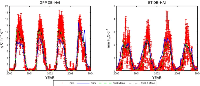
Some of the feedbacks between vegetation and climate have been studied in the Euro-Mediterranean area using both models and data.

The Lund-Potsdam-Jena (LPJ) Dynamic Global Vegetation Model describes the water, carbon, and energy exchange between land surface and atmosphere by means of a given set of parameters and input variables. In order to retrieve the underling probability density function of some key-model parameters controlling water and carbon cycle as well as to improve the efficiency of LPJ to simulate water and carbon fluxes a data assimilation system has been developed; it is based on a Bayesian approach that consistently combines prior knowledge about parameters with observations. Daily values of evapotranspiration and gross primary production, measured with eddy covariance technique in ten different CarboeuropeIP sites, have been compared with modeled data in order to constrain parameter values and uncertainties.

Results show how data assimilation is a useful tool to improve the ability of the model to simulate correctly water and carbon fluxes at local scale: after the inversion, in fact, LPJ successfully matches the observed seasonal cycle of the diverse fluxes, and corrects for the prior misfit to day-time GPP and ET.

The impact of land cover change on regional climate have been analyzed using the mesoscale model RegCM3. Three different simulations have been performed to asses the effects of an hypothetical deforestation and afforestation on climate.

Results show how land cover changes have a substantial impact on dynamic and thermodynamic, and how also area does not affected by land cover changes shows a significant variability in some climatic fields. Finally, the land cover changes have an important impact on the extreme events.

This thesis highlights how vegetation dynamics and climate influence each other. For such reason to improve simulation results we should develop fully coupled models that take into account some of the most important feedbacks between land surface and atmosphere.

CONTENTS

Abstract

1

INTRODUCTION

1.1 Background 1

1.2 Objectives of this thesis 2

2

LAND SURFACE-CLIMATE INTERACTIONS

2.1 Land surface processes 4

2.2 The role of terrestrial biosphere on the global carbon cycle 8 2.3 Dynamic Global Vegetation Models 14 2.4 The concept of data assimilation 19

3

A BAYESIAN INVERSION OF LPJ DYNAMIC GLOBAL

VEGETATION MODEL

3.1 Introduction 22

3.2 Methods and Data: An implementation of a data assimilation system into LPJ 24

3.2.1 Optimization algorithms 24

3.2.1.1 Conjugate gradient methods 25 3.2.1.2 Metropolis Algorithm 29

3.2.2 The optimization schemes 33

3.2.3 Model description and input data 35 3.2.4 Initial model parameters values and prior uncertainties 41 3.2.5 Eddy-covariance flux data 46 3.3 Results: Changes in model parameters and fluxes after a Monte Carlo sampling 52

3.3.1 Introduction 52 3.3.2 Comparing different optimization strategies and performances 53

Contents iv

3.3.3 Effect of the different parameterizations on water and carbon fluxes 58 3.3.4 Interstation and interannual variability 65 3.3.5 Final-optimized parameters and uncertainty 72 3.3.6 Validation against eddy data for year 2003 76 3.3.7 Global effects of the new parameterization 79

3.4 Discussions and conclusions 87

4

EFFECTS OF LAND COVER CHANGES ON CLIMATE OVER

EURO MEDITERRANEAN AREA

4.1 Introduction 91

4.2 Model, data, and experimental setup 93

4.2.1 Model description 93

4.2.2 Potential vegetation 94

4.3 Results: Impacts of land cover change on climate 97 4.3.1 Comparison of domain-averaged climate 97 4.3.2 Spatial differences in seasonally surface climate 98 4.3.3 Differences in atmospheric circulation 104

4.3.4 Impact on extreme events 105

4.4 Discussions and conclusions 107

Appendix

I

INTRODUCTION

1.1

BACKGROUND

Over the last decades both model and observational studies have shown that the climate system is sensitive to the processes that characterize the earth’s continental surface and that an accurate representation of these processes in climate models is of great importance [Alessandri et al., 2007]. However, even if the interaction between atmosphere and land surface systems is an essential aspect for climate studies many uncertainties are still remaining, due to an inadequate understanding of all the processes and complex interactions involved.

The models of the coupled climate-carbon cycle system, on one hand, vary widely in predictions of future CO2 sinks [Friedlingstein et al., 2006]. The strength of this sink, which consists uptake through terrestrial ecosystems and the oceans, has important implications for creating emissions targets to reduce the likelihood of dangerous anthropogenic interference in the climate system. Thus, policy decisions must be made in the face of large uncertainties. By assimilating measurement of CO2 fluxes into process-based biogeochemical models, we can constrain some model parameters and also decrease the misfit between simulation results and observations; this step could lead to a reduction of the uncertainty in future predictions, and hence we should be able to deliver good estimates of the carbon sinks and sources.

On the other hand, an improved knowledge and description of land surface water, energy and carbon conditions plays a pivotal role for improving land ecosystem and climate prediction. For example, soil moisture is a crucial variable for climate models because it influences the partitioning of available energy into sensible and latent heat fluxes and hence the evolution of the lower atmospheric conditions.

During the last few years, soil-vegetation schemes coupled to global climate models have become a fundamental tool to improve our knowledge of these processes. Global Circulation Models (GCMs) have been used to describe soil–atmosphere interactions and feedbacks in a

1.1 Background 2

wide variety of climatic conditions, including studies related to climate change. More recently, Regional Climate Models (RCMs) have also started to be used for these studies. Regional numerical models are an interesting tool to analyze surface processes highly related to regional scales, as many of the aspects related to hydrology and surface water budget mechanisms, and their transmission to the free atmosphere through the boundary layer. Thus, regional climate models have been used to study impacts of deforestation processes, changes in land-use, local and non-local changes in precipitation due to soil moisture modifications, initial soil moisture conditions influence on precipitation for long time periods (even months), relations of soil moisture and rainfall for drought or flood conditions, impacts of regional anthropogenic vegetation changes.

The results of these studies suggest that the feedbacks between land surface and atmosphere are key determinants of climate at a range of spatial (local to global) and temporal (seasonal to centennial) scales. In fact, many of the properties involved (vegetation type and cover, soil moisture, and snow cover) evolve continuously in response to atmospheric-climatic forcing, while the initial forcing may be amplified or dampened as a consequence of their interaction. For such reason, the necessity of more realistic and accurate computations of the exchanges of energy, momentum, water and carbon between the land surface and the atmosphere has been leading to continuous developments in land surface models. A parameterization of the vegetation included in the global circulation models or in the regional climate models allow us to better simulate the evolution of surface parameters such as roughness length, albedo, and surface–soil moisture [Alessandri et al., 2007]. Furthermore, the inclusion of a realistic vegetation allows a description of the function of roots, of the physiological control of transpiration, and of the water interception by the vegetation canopies, which is quickly evaporated back to the atmosphere and this can improve our simulation results.

1.2

OBJECTIVES OF THIS THESIS

The aim of this Ph.D. thesis is to study some of the feedbacks between vegetation and climate in the Euro-Mediterranean area using both models and data. More precisely, two different studies have been performed: in the first case have a data assimilation system have been developed to constrain some model parameters controlling the exchange of water and carbon fluxes between vegetation and atmosphere, while in the latter case is analyzed how theoretical land cover changes affect the climate.

1.2 Objectives of this thesis 3

To improve our knowledge on the influence of local-climate conditions on the parameterization of some model processes, we constrained twelve relevant LPJ dynamic global vegetation model parameters controlling water and carbon cycle; this allowed as well to minimize the mismatch between simulations results and measurement of water and carbon fluxes in the Euro-Mediterranean area. The improved knowledge of present-day parameter variability can be used in future to improve regional scenario simulations for the 21st century.

To achieve this objective we used multiple sites eddy data from the CarboEuropeIP network to develop a framework for nonlinear parameter estimation and to retrieve the shape of the underlying probability density function (PDF) of twelve model parameters controlling photosynthesis and evapotraspiration in the Lund-Potsdam-Jena Dynamic Global Vegetation Model (LPJ-DGVM) [Sitch et al., 2003]. The results of the multi sites optimization are used to analyze the spatial variability of parameters within and between different PFTs, and also to find out possible systematic defects in the model parameterization.

The analyses of parameter distribution as a function of dominant vegetation and climate, and in comparison to prior knowledge about the parameters from leaf-level will advance our understanding of how global models can represent specific processes of different ecosystems. Our hypotheses are:

1) that parameters of the Farquhar model of photosynthesis, and of water uptake and potential evapotranspiration change only slightly at ecosystem scale and between sites with the same vegetation type or climate forcing.

2) that the coupling between carbon and water fluxes through canopy conductance is reliable by the LPJ-DGVM.

On the other hand, to evaluate how the vegetation affect the climate, different simulation that make use of some hypothetical land cover changes have been performed by mean of a regional climate model (RegCM3) [Giorgi et al., 1990; Giorgi et al., 1993a, b]. In mesoscale models the land surface represents the lowest limit of the atmosphere, but the vegetation dynamics have been poorly described. For such reason here we focus on the effect of the changes in vegetation coverage on climate

The structure of the thesis is as follows. In the chapter 2 will be briefly discussed the main interactions between terrestrial ecosystems and atmosphere. In Chapter 3 will be described the construction and application of a data assimilation system, while in Chapter 4 will be evaluated the impact of theoretical land cover change on climate.

II

LAND SURFACE-CLIMATE

INTERACTIONS

2.1

LAND SURFACE PROCESSES: TERRESTRIAL

ECOSYSTEMS-ATMOSPHERE INTERACTIONS

Terrestrial ecosystems-atmosphere interactions refer to exchange of heat, moisture, traces gases, aerosols, and momentum between land surfaces and the overlying air [Pielke et al, 1998].

Terrestrial ecosystems and climate influences one another on timescale ranging from seconds to millions of years [Sellers et al., 1995; Pielke et al., 1998]. Ecosystems influence weather and climate over period of seconds to years trough exchanges of energy, moisture, and momentum between the land surface and the atmosphere and the changes in global-scale atmospheric circulation that can result from changes in these fluxes [Pielke et al., 1998]. Ecosystem structure and function is strongly determined on timescales of decades to centuries by climate influences, primarily through temperature ranges and water availability. On timescales of thousands of years, glacial-interglacial cycles probably involve coupled changes in the geographical distribution of the terrestrial ecosystems, surface albedo, biogeochemical cycling, and climate in response to changing solar forcing. On even longer geological timescales (millions of years), terrestrial ecosystems and the Earth’s climate have evolved together through such mechanisms as changes in the biochemistry and the composition of the atmosphere [Pielke et al., 1998].

Land covers about 30% of the surface area of the Earth; the land surface is considered as the lower level for the planetary boundary layer (PBL). The PBL represent the lowest part of the troposphere, where wind, temperature, and humidity are strongly influenced by the surface processes. These processes are so tightly intertwined that they cannot be treated separately. Net radiation is partitioned primarily among three major avenues of energy exchange between the

2.1 Land surface processes: terrestrial ecosystems-atmosphere interactions 5

ecosystem and the atmosphere: ground heat flux, latent heat flux and sensible heat flux [Chapin

et al., 2002].

The ground heat flux represents the heat transferred from the surface into and out of the soil; it is negligible over a day in most temperate and tropical ecosystems because the heat conducted into the soil during the day is balanced by heat conducted back to the surface at night. The magnitude of ground heat flux depends on the thermal gradient between the soil surface and deep soils and the thermal conductivity of soils, which is greatest in soils that are wet and have a high bulk density. In contrast to the temperate soils, permafrost regions of the arctic and boreal forest have substantial ground heat flux, due to the strong thermal gradient between the soil surface and the permafrost [Chapin et al., 2002].

Solar energy drives also the hydrological cycle thought the vertical transfer of water from Earth to the atmosphere via evapotranspiration (or latent heat), the sum of evaporation from surface and transpiration, which is the water loss by plants. So, the latent heat flux is the energy transferred to the atmosphere when water is transpired by plants or evaporates from leaf or soil surfaces. This heat is transported from the surface into the atmosphere by convection. Evapotranspiration accounts for 75% of the turbulent energy transfer from the Earth to the atmosphere and is therefore a key process in Earth’s energy [Chapin et al., 2002].

Finally, sensible heat flux is the heat that is initially transferred to the near-surface atmosphere by conduction and to the bulk atmosphere by convection: it is controlled in part by the temperature differential between the surface and the overlying air. Air close to the surface becomes warmer and more buoyant than the air immediately above it, causing this parcel of air to rise. Mechanical turbulence is caused by winds blowing across a rough surface: it generates eddies that transport warm moist air away from the surface and bring cooler drier air from the bulk atmosphere back toward the surface. Surface turbulence is the major process that transfers latent and sensible heat between the surface and the atmosphere [Chapin et al., 2002].

There are important interactions between latent and sensible heat fluxes from ecosystems. The consumption of heat by the evaporation of water cools the surface, thereby reducing the temperature differential between the surface and the air that drives sensible heat flux. Conversely, the warming of surface air by sensible heat flux increases the quantity of water vapour that the air can hold and causes convective movement of moist air away from the evaporating surfaces. Both of these processes increase the vapour pressure gradient that drives evaporation. Because of these interdependencies, surface moisture has a strong effect on the Bowen ratio-that is, the ratio of sensible to latent heat flux [Chapin et al., 2002].

Bowen ratios range from less than 0.1 for tropical oceans to great than 10 for deserts, indicating that either latent heat flux or sensible heat flux can dominate the turbulent energy transfer from

2.1 Land surface processes: terrestrial ecosystems-atmosphere interactions 6

ecosystems to the atmosphere, depending on the nature of the ecosystem and the climate. In general, ecosystems with abundant moisture have higher rates of evapotranspiration and therefore lower Bowen ratios than do dry ecosystems. Similarly, ecosystems dominated by rapidly growing plants, which have high transpiration rates, have proportionately lower sensible heat fluxes and low Bowen ratios. Strong winds and/or rough canopies, which generate surface turbulence, tend to prevent a temperature build-up at the surface and therefore reduce sensible heat flux and Bowen ratio. For these reasons, energy partitioning varies substantially both seasonally and among ecosystems. The Bowen ratio determines the strength of the linkage between the energy budget and the hydrologic cycle, because it is inversely related to the proportion of net radiation that drives water loss from ecosystems: the lower the Bowen ratio, the tighter the linkage between the energy budget and the hydrologic cycle [Chapin et al., 2002].

Besides influencing the atmosphere by transpiration and the associated partitioning of surface heat fluxes into latent and sensible contributions, vegetation also affects the surface albedo and the roughness length [Heck et al, 2001].

The albedo over vegetated land surfaces can vary from very low values (10-15% over humid tropical forests) to somewhat larger values (15-20% over herbaceous vegetation) [Hartmann, 1994]. The vegetation albedo is a function of plant structural and optical properties and the leaf area index [Dickinson, 1983]. As the amount of leaf area increases, light absorption increases inside a canopy and the reflection from background soil decreases. This results in an overall decrease in surface albedo. A similar situation is observed in the case of snow in tree-covered landscapes. Land surface with fully covered snow has high values of surface albedo (~0.8). The high albedo is masked in the presence of trees and can reach significantly lower values (~0.2-0.4) depending on vegetation cover type.

The roughness of a canopy surface influences the partitioning of sensible and latent heat fluxes between the land surface and the overlying air. Changes in vegetation height and leaf area exert a larger drag force on the atmospheric boundary layer and this influences the atmosphere dynamically as winds blow over the land's surface. Roughness is determined by both topography and vegetation [Hartmann, 1994].

Besides vegetation, also soils play a pivotal role representing an important seasonal water reservoir for the hydrological cycle. In midlatitudes soil plays a similar role to that of the oceans, but instead of storing heat, it stores precipitation in winter, which moistens then the atmosphere in summer via evapotranspiration [Heck et al, 2001]. The associated seasonal storage of water in the soil introduces long-term memory effects with timescales of several months which interact with the typical atmospheric timescales of few days.

2.1 Land surface processes: terrestrial ecosystems-atmosphere interactions 7

The study of the feedback mechanisms of the coupled land-atmosphere system has become increasingly important in recent years [Entekhabi, 1995; Betts et al., 1996], and their numerical parameterizations in atmospheric models become more and more refined [e.g., Dickinson et al., 1986; Sellers et al. 1986]. Extensive, satellite-based data sets are currently used to describe land surface parameters and monitor their seasonal and interannual variations. Feedback mechanisms between the land and the atmosphere are also relevant to climate change issues, since they may modulate and interact with anthropogenic changes. Anthropogenic CO2 emissions and the associated temperature changes [Houghton et al., 1995] may affect the physiological characterization of plants species [Sellers et al., 1996; Betts et al., 1997; Bounoua et al., 1999;

Heck et al, 2001].

General circulation models and regional climate models have increasingly been used to investigate the atmospheric and climate response to imposed global or regional changes of surface parameters (e.g., tropical deforestation, see Heck et al. [2001] for detailed references). Modeling of meteorological flows requires the use of conservation equations for fluid velocity, heat, mass of dry air, water substance in its three phases, and many other natural and anthropogenic atmospheric constituents. The characterization of biospheric processes in these models, however, has been limited to simple representation where most aspects of the soil and vegetation are prescribed. Stomatal conductance responds to atmospheric inputs of solar radiation, air temperature, air relative humidity, precipitation, air carbon dioxide concentration, and to soil temperature and moisture. Till few years ago, in meteorological models, these were the only meteorological variables to which the vegetation ant the soil dynamically respond [Pielke et al, 1998].

The last generation of GCM and RCM has a complex vegetation or its fully coupled with a complex land surface model. Current GCM and RCM, however, also lack dynamical vegetation and carbon cycling, so are unable to take account of feedbacks related to the evolution of vegetation structure, composition and growth as conditions change. The effects of regional-to-global feedbacks are highly relevant when assessing the carbon cycle and the greenhouse gasses forcing and can be a significant source of uncertainty [Morales et al., 2007].

The modeling of terrestrial ecosystems involves the short-term response of vegetation and soils to atmospheric effects, and the longer-term evolution of species composition, biome dynamics, and nutrient cycling associated with landscape and soil structure changes. The assimilation of carbon resulting in the growth of vegetation, and its subsequent release during decay has been a focus of these models. The spatial scale of these simulations have ranges from patch size (microscale) to biome (mesoscale) scales.

2.2 The role of terrestrial biosphere on the global carbon cycle 8

2.2

THE ROLE OF TERRESTRIAL BIOSPHERE ON THE GLOBAL

CARBON CYCLE

Carbon dioxide (CO2) is a naturally abundant trace gas in the atmosphere. Through its radiative properties it is (besides atmospheric water vapour) the most important greenhouse gas. Because of the natural greenhouse effect the mean global surface temperature amounts to around +15 ◦C compared to -18 ◦C without any climate relevant trace gases in the atmosphere and therefore is a necessity for our life on earth.

Although many elements are essential to living matter, carbon is the key element of life on Earth. The biogeochemical cycle of carbon is necessarily very complex, since it includes all life forms on Earth as well as the inorganic carbon reservoirs and the link between them. So, to understand and project future changes in the global carbon cycle, it is necessary to understand its underlying elements and processes.

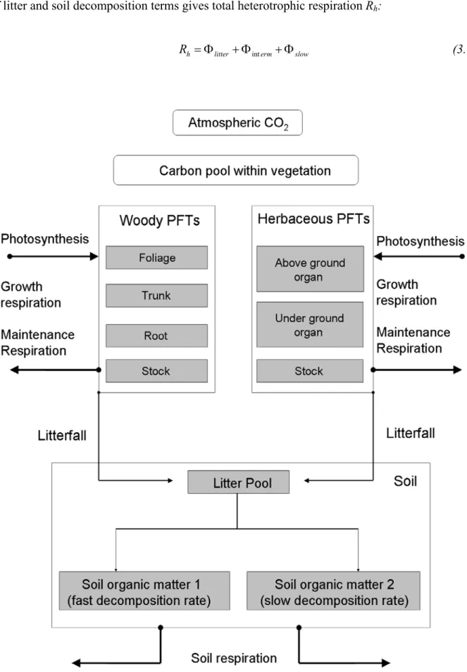
The carbon cycle consists of three main compartments (Figure 2.1): the atmosphere, the oceans,

and the biosphere. Each compartment consists of different carbon pools and exchanges carbon at different rates.

Figure 2.1. The global carbon cycle for the 1990s, showing the main annual fluxes in PgC yr–1:

pre-industrial ‘natural’ fluxes in black and ‘anthropogenic’ fluxes in red. Within the boxes, black numbers give the preindustrial size of the reservoirs and red numbers denote the changes resulting from human activities since preindustrial times. For the land sink, the first red number

is an inferred terrestrial land sink whose origin is speculative; the second one is the decrease due to the deforestation (taken from Denman et al. [2007]).

2.2 The role of terrestrial biosphere on the global carbon cycle 9

The largest amount of carbon (C) by far (about 38,000 Pg C) [Gruber et al., 2004] is stored in

the middle and deep ocean (Figure 2.1). This C is, however, relatively inert and, as such, less

relevant for the C cycle in coming decades [Bolin et al., 2000; Gruber et al., 2004]. Smaller but still considerably large pools are found in the terrestrial biosphere (2100–3000 Pg C), the surface layer of the oceans (600 Pg C) and the atmosphere (700–800 Pg C) [Grace, 2004; Denman et al., 2007].

Numerous well-replicated measurements of the composition of air bubbles trapped in Antarctic ice showed that the atmospheric CO2 concentration remained relatively constant at a level of about 280 parts per million (ppm) [Indermühle et al., 1999] during the last 10.000 years suggesting that the carbon cycle has been in quasi-equilibrium during that time.

Since industrialization (the last ≈150 years) atmospheric CO2 concentration increased by more than 80 ppmv to a total value of around 370 ppmv today, a magnitude which has not been exceeded during the last 420.000 years at a rate which is unique for at least the last 20.000 years [Prentice et al., 2001].

Fossil fuel burning and related industrial activities, as well as terrestrial carbon losses from land-use change are the caland-uses for the rise in atmospheric carbon concentration. Atmospheric CO2 is, however, increasing only at about half the rate of fossil fuel emissions; the rest of the CO2 emitted either dissolves in sea water and mixes into the deep ocean, or is taken up by terrestrial ecosystems [Prentice et al., 2001]. Partitioning of the terrestrial and ocean fluxes based on simultaneous measurements of CO2 and O2 suggest that the terrestrial biosphere sequesters up to 30% of the fossil-fuel emissions [Ciais et al., 1995; Prentice et al., 2001; House et al., 2003]. Because of the pivotal role that carbon plays in the climate system it is critical that we understand all the processes that regulate its cycling through vegetation and develop such mechanisms into GCM in order to make good estimates on the future changes in the global

carbon cycle.

The CO2 uptake and release of the terrestrial biosphere is determined by a number of processes

that are sensitive to climate, atmospheric CO2, moisture availability, and land use. Within the

terrestrial biosphere, plants take up CO2 by diffusion through the stomata of leaves (globally

about 270 Pg C yr-1) [Ciais et al., 1997]. More than 50% of this CO2 diffuses back to the

atmosphere without becoming part of biogeochemical processes within plants. A basic

biogeochemical process within plants is photosynthesis, where CO2 is converted under the

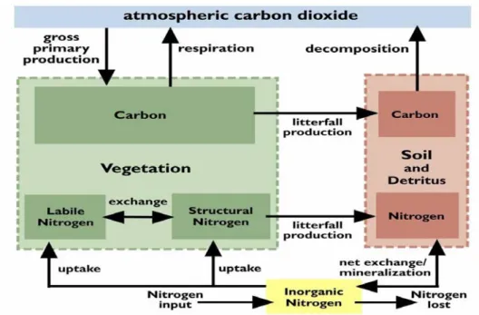
influence of “active radiation” (400-700 nm wave length) into carbohydrates that serve as raw material for further processes. The amount of C that is fixed through photosynthesis is called Gross Primary Production (GPP, Figure 2.2). The amount that is really taken up by plants, allocated to and incorporated in new plant tissues is defined as Net Primary Production (NPP,

2.2 The role of terrestrial biosphere on the global carbon cycle 10

Figure 2.2). As such NPP includes all increments in the biomass of leaves, stems, branches, roots, and reproductive organs. The remaining part of the C is lost by autotrophic respiration (Ra, Figure 2.2). Most of the C fixed through NPP also returns back to the atmosphere through heterotrophic respiration (Rh, Figure 2.2), and disturbances. The former process is the decomposition of soil organic matter by bacteria and fungi, which consume most of the organic material that enters the soil through dying plant material. Several soil C pools can be distinguished with different C contents, chemical composition, and different bacteria and fungi

composition. As result they have often different decomposition rates. The difference between Rh

and NPP is called Net Ecosystem Productivity (NEP) or Net Ecosystem exchange (NEE, Figure

2.2). Negative fluxes denote a net carbon flux from the atmosphere to the terrestrial biosphere because the assimilation process dominate on respiration terms; in such case the ecosystem is considered a sink of carbon. It represents the amount of carbon that is annually stored in the terrestrial biosphere. When also accounting for C losses due to fires, land-use change, harvest, and erosion, the total C flux is called Net Biome Productivity (NBP).

Figure 2.2. Main component of the terrestrial carbon cycle; blue arrows denote an assimilation of carbon by vegetation, while red arrows point out an emission of carbon from ecosystem to

atmosphere.

Globally, the terrestrial biosphere stores about 2100–3000 Pg C, divided into 466–660 Pg C in the vegetation and 1460–2300 Pg C in soils. The total terrestrial C storage is about three times

2.2 The role of terrestrial biosphere on the global carbon cycle 11

the amount in the atmosphere and the surface layer of the ocean [Sabine et al., 2004; Denman et al., 2007]. The range is caused, for example, by differences in definitions (e.g. some soil compartments), the total area included and various uncertainties (especially related to the soil carbon budget, which is difficult to measure). Global annual terrestrial GPP is estimated at 120

Pg C yr-1 [Denman et al., 2007]. Roughly, one half of this gross primary production is lost to the

atmosphere via autotrophic respiration from plant tissues [Lloyd and Farquhar, 1996; Waring et

al., 1998], and the remaining 53–68 Pg C yr-1 Pg C are incorporated into plant tissue as terrestrial net primary production

The estimates are based on integration of field measurements, remote sensing, atmospheric measurements and modeling the historical C cycle. The range is due to uncertainties in land cover and land use [Houghton, 2003; Lambin et al., 2003], and in the response of the terrestrial

biosphere to environmental changes like climate, CO2, and nitrogen fertilization.

NPP fluxes vary with the study, especially for tropical regions [Berthelot et al., 2005]. Furthermore, the range is caused by the different measurement methods and the different time periods of the studies. Regarding the time period, Potter et al. [1999] and Nemani et al. [2003] showed that the global NPP increased about 6% over the last decades. The global NEP flux over

the last decades is estimated at between -3 and -10 Pg C yr-1 [Watson et al., 2000; Cox, 2001;

Cramer et al., 2001; Prentice et al., 2001; Grace, 2004; Schaphoff et al., 2006]. Note that there is a wide range of uncertainty, especially in soil processes [Grace, 2004], and a considerable inter-annual variability [Valentini et al., 2000]. Furthermore, the low end of the range often represents model results that implicitly include some effects of disturbances.

Looking at the possible future, we see that various models have projected an increasing NEP flux up to the middle of this century, followed by a stabilization [Cramer et al., 2001; Scholes and Noble, 2001], a decline [Lucht et al., 2006; Schaphoff et al., 2006] or even a shift towards a C source [Cox et al., 2004]. The decrease (and shifts towards a C source) is due the enhanced heterotrophic respiration due to the increased mean atmospheric temperature. These projections are also surrounded with substantial uncertainty due to uncertainties in future regional climate

[Schaphoff et al., 2006] and the response of the biosphere to future climate and atmospheric CO2

[Cramer et al., 2001; Friedlingstein et al., 2006].

When CO2 emissions due to land-use changes are excluded, the global residual terrestrial C sink

is estimated to be in the range of -0.9 to -2.4 Pg C yr-1 over the 1980s and -2 to -3 Pg C yr-1 in

the 1990s [Denman et al., 2007]. Recent observations indicate that the global sink is still

2.2 The role of terrestrial biosphere on the global carbon cycle 12

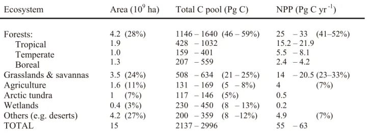
The C pools and fluxes are not homogenously distributed across the world, but differ

geographically, seasonally and between ecosystem types (Table 2.1). Ecosystem types that store

large quantities of C are forests, grasslands, and wetlands.

Ecosystem Area (109 ha) Total C pool (Pg C) NPP (Pg C yr -1) Forests: Tropical Temperate Boreal 4.2 (28%) 1.9 1.0 1.3 1146 – 1640 (46 – 59%) 428 – 1032 159 – 401 207 – 559 25 – 33 (41–52%) 15.2 – 21.9 5.5 – 8.1 2.4 – 4.2

Grasslands & savannas 3.5 (24%) 508 – 634 (21 – 25%) 14 – 20.5 (23–33%)

Agriculture 1.6 (11%) 131 – 169 (5 – 8%) 4 (7%)

Arctic tundra 1 (7%) 117 – 146 (5%) 0.5

Wetlands 0.4 (3%) 230 – 450 (8 – 13%) 0.2

Others (e.g. deserts) 4.2 (27%) 200 – 359 (8 –12%) 4.9 (7%)

TOTAL 15 2137 – 2996 55 – 63

Table 2.1. Global C pools and NPP fluxes differentiated over ecosystems (sources: Silver

[1998]; Gitay et al. [2001]; Nemani et al. [2003]; Grace [2004]; Sabine et al. [2004]; Fischlin et al. [2007]).

On the global scale, forests cover more than 4 billion hectares or about 28% of the terrestrial biosphere [FAO, 2001; Grace, 2004]. About half the forest area is located in developed countries (mostly temperate and boreal types of forests) and half in developing (mostly tropical) countries. Forest ecosystems play a pivotal role in the global C cycle because they store nearly half the

terrestrial C (Table 2.1). If considering only the vegetation C pools, forests even store 80–90% of

the carbon [Körner, 2003]. The largest fraction of this pool (i.e. about 60%) is stored in tropical forests [Sabine et al., 2004]. Note that the C pools and fluxes vary even considerably between tropical forest types, depending on the type of forest and degree of disturbance. The living

biomass of tropical rain forests, for example, ranges between 160–190 Pg C ha-1 compared to dry

forests with only 30–60 Pg C ha-1. Boreal forests also contain a considerable amount of carbon in

the soil (i.e. 200–500 Pg C) [Sabine et al., 2004].

Secondly, forest ecosystems are important for the global C cycle because of the considerable C exchange between forests and the atmosphere. Almost all the forests around the world currently

sequester C and, in particular, tropical forests fix into biomass up to 1200 gC m-2 yr-1. Including

the C losses due to deforestation, tropical forests still represent either a small C sink [Hougton, 2002; Cramer et al., 2004; Grace, 2004].

2.2 The role of terrestrial biosphere on the global carbon cycle 13

Natural grasslands are also widely spread across the world. The total grassland area is about 3.5 billion hectares, of which 65% is located in warm and tropical regions [Sabine et al., 2004]. Much grassland around the world has been converted into agricultural land over the past decades, resulting in a declining amount [Meyer and Turner, 1998]. Natural grasslands are important for the global C cycle because of the large extent and the considerable carbon storage, on the one hand, and their sensitivity to climate change and direct human influence on the other [Parton et al., 1994]. Regarding the former, the global C storage in the living biomass of natural grasslands is 33–85 Pg C, while the total C pool in grassland soils is in the range of 279 and 559 Pg C [Sabine et al., 2004]. Large differences are found across the world for grasslands too. The C storage in the living biomass of tropical grasslands is generally higher than in grasslands in temperate regions, whereas the soil C pools are comparable in both parts of the world [Sabine et al., 2004]. Global NPP estimates of grasslands vary between 8.6 and 15 Pg C yr-1. The productivity decreases due to human influences, causing a reduced C storage and soil erosion [Burke et al., 1991; Ojima et al., 1993]. The observed NPP range is, in particular, determined by the seasonal distribution of precipitation [Ojima et al., 1993]. This is because many natural grasslands in the world are water limited [Meyer and Turner, 1998]. Because of the dependency on water, climate change (especially seasonality and precipitation) may have a considerable effect on the total C balance of grasslands.

Wetlands also store large amounts of carbon, mainly in soils (240–455 Pg C) [Gorham, 1991; Sabine et al., 2004]. The majority of the wetlands and C storage can be found in boreal and arctic regions. Tropical wetlands are less relevant (total C storage about 70 Pg C) [Diemont, 1994], although the largest C densities have been observed here. Furthermore, wetlands are important for the C cycle because of the risk of a significant loss of their soil C pool under climate change. The optimum annual average temperature for C sequestration of most wetlands is between 4 and

10 oC. This can be currently observed in much of the southern-boreal and northern-temperate

zones. With projected temperature increases, conditions are likely to exceed the optimum range. Numerous arctic wetlands may even disappear entirely under temperate increases in the range of

2–3 oC [Hitz and Smith, 2004]. Likewise, changes in precipitation affect the species composition

of wetlands and, as such, the functioning [Keddy, 2000]. All these changes can result in a change in wetlands from a C sink into a C source.

Understanding the complexity of the terrestrial C dynamics in relation to anthropogenic activities and environmental changes, including future trends and assessment of possible policies, can be achieved through modeling. Various types of terrestrial C-cycle models have been developed, ranging from highly aggregated and simple, to complex process-based. Next section will give a brief description of the existing models.

2.3 Dynamic Global Vegetation Models 14

2.3

DYNAMIC GLOBAL VEGETATION MODELS

To formulate a model is to put together pierces of knowledge about a particular system into a consistent pattern that can form the basis for (1) interpretation of the past history of the system and (2) prediction of the future of the system. In other words, simulation models use mathematical expressions to describe the behaviour of a system in an abstract manner [Bratley et al., 1987]. The mathematical expressions are based on scientific theories and assumptions. Compared to the real world, the structure and processes are simplified in any simulation model. Simulation models have also other diverse purposes from predictions/projections (i.e. assessing responses to changing driving forces) described above such as education and an improved understanding/discovery of relationships between the elements of a system [Goudriaan et al., 1999]. Furthermore, a general purpose of any model is to enable its users to draw conclusions about the real system by studying and analyzing the model results.

The complexity of ecological controls over all the processes that influence ecosystem carbon balance makes long-term projections of terrestrial carbon storage a daunting task. Making these projections is, however, critical to improving our understanding of the relative role of terrestrial ecosystems in the global carbon balance. Experiments that test the multiple combinations of environmental conditions influencing terrestrial carbon storage are difficult to design. Modeling allows a limited amount of empirical information to be greatly extended through simulation of complex combinations of environmental-biotic interactions [Chapin et al., 2002]. One important use of ecosystem models has been to identify the key controls that govern rate estimates of the area of each patch type. Satellite imagery now provides improved estimates of the aerial extent of many patch types, but spatial and temporal variation in processes makes it difficult to find good representative sites from which data can be extrapolated [Chapin et al., 2002]. This extrapolation approach can be combined with empirical regression relationships (rather than a single representative value) to estimate process rates for each patch type. Carbon pools in forests, for example, might be estimated as a function of temperature or normalized difference vegetation index (NDVI) rather than assuming that a single value could represent the carbon stocks of all forests.

Process-based models make up another approach to estimating fluxes or pools over large areas. These estimates are based on maps of input variables for an area (e.g., maps of climate, elevation, soils, and satellite-based indices of leaf area) and a model that relates input variables to the ecosystem property that is simulated by the model.

2.3 Dynamic Global Vegetation Models 15

Many of key processes regulating NEP involve changes that occur over decades to centuries (Figure 2.3). The temporal resolution of the models must therefore be coarse, with time steps (the shortest unit of time simulated by the model) of a day, month, or year. Use of relatively long time steps such as weeks or months reduces the level of detail that can be considered.

Figure 2.3. Spatial and temporal resolution of environmental processes (left panel) and carbon cycle dynamics (right panel).

The basic structure of a model of NEP must include the pools of carbon in the soils and vegetation. It must also include the fluxes of carbon from the atmosphere to plants (GPP or NPP), from plants to the atmosphere (plant respiration, harvest, and combustion), from plants to soil (litter fall), and from soil to the atmosphere (decomposition and disturbance). Models differ in the detail with which these and other pools and fluxes are represented. Plants, for example, might be considered a single pool or might be separated into different plant parts (leaves, stems, and roots), functional types of plants (e.g., trees and grasses in a savanna), or chemical fractions such as cell wall and cell contents.

So far, a broad range of models exist, and they are used to investigate the magnitude and geographical distribution of a wide numbers of variables related to the vegetation [Cramer et al., 1999]. These models range in complexity from regressions between climatic variables and one or more estimates. Different models use different simplifying assumptions, and they often use

2.3 Dynamic Global Vegetation Models 16

different environmental variables leading to different estimates. So, there is no single "best" model, but each model has a unique set of objectives, and the model structure must be designed to meet these objectives.

Perhaps the biggest challenge in model development is deciding which processes to include. One approach is to use a hierarchical series of models to address different questions at different scales. Models of leaf-level photosynthesis and of microclimate within a canopy have been developed and extensively tested for agricultural crops, based on the basic principles of leaf biochemistry and the physics of radiation transfer within canopies. One output of these models is a regression relationship between environment at the top of the canopy and net photosynthesis by the canopy. This environment-photosynthesis regression relationship can then be incorporated into models operating at larger temporal and spatial scales to simulate NPP, without explicitly including all the details of biochemistry and radiation transfer. This hierarchical approach to modeling provides an opportunity to validate the model output (i.e., compare the model predictions with data obtained from field observations or experimental manipulations) at several scales of temporal and spatial resolution, providing confidence that the model captures the important underlying processes at each level of resolution.

Global vegetation models (GVM) have in the past decade evolved from largely statistical correlation to more process-based, rendering greater confidence in their abilities to address questions of global change. There are generally two classes of GVMs, biogeography models and biogeochemistry models [Haxeltine and Prentice, 1996]: biogeochemistry models have traditionally been used to assess biogeochemical fluxes through ecosystem given prescribed distribution of ecosystem types, while biogeography models have been used to simulate the response of biome boundaries to projected changes in climate and atmospheric CO2 [Pan et al., 2002]. In other words, the biogeography models place emphasis on determination of what can live where, but either do not calculate or only partially calculate the cycling of carbon and nutrients within ecosystems. The biogeochemistry models simulate the carbon and nutrient cycles within ecosystems, but lack the ability to determine what kind of vegetation could live at a given location under specific environmental conditions.

As biogeochemistry model, the Terrestrial Ecosystem Models (TEMs) were designed to simulate the carbon budget of ecosystems for all locations on Earth at 0.5° longitude by 0.5° latitude resolution (60000 grid cells) for time periods of a century or more [McGuire et al., 2001]. TEM has a relatively simple structure and a monthly time step, so it can run efficiently in large numbers of grid cells for long periods of time. Soil, for example, consists of a single carbon pool. The model assumes simple universal relationships between environment and ecosystem processes based on general principles that have been established in ecosystem studies. The

2.3 Dynamic Global Vegetation Models 17

model assumes, for example, that decomposition rate of the soil carbon pool depends on the size of this pool and is influenced by the temperature, moisture, and C:N ratio of the soil. TEM incorporates feedbacks that constrain the possible model outcomes. The nitrogen released by decomposition, for example, determines the nitrogen available for NPP which in turn governs carbon inputs to the soil and therefore the pool of soil carbon available for decomposition. This simplified representation of ecosystem carbon dynamics is sufficient to capture global patterns of carbon storage [McGuire et al., 2001], making the model useful in simulating regional and global patterns of soil carbon storage. The basic structure of a TEM is shown in Figure 2.4.

Figure 2.4. Driven from monthly climatology, TEM simulates the terrestrial carbon cycle.

To develop regional and global estimates of NPP and carbon storage, TEM normally uses geographically-referenced data sets organized at a spatial resolution of 0.5x0.5 degree to capture the spatial variability of environmental conditions across the region. Because a 0.5 degree grid cell covers a large area and environmental conditions are considered to be constant within the grid cell, NPP estimates might be improved using data sets with a finer spatial resolution.

As a matter of fact, even in a constant climate, ecosystem structure is generally unstable. Natural mortality of plants or of plant parts such as leaves and branches constantly adds biomass to the litter pool upon which other organisms thrive and thereby influence the flux of carbon from organic substances back to the atmosphere. This mortality occurs erratically, usually as a result of disturbances, and thereby creates new opportunities for other plants. Later stages of the process, such as the decomposition of dead plant matter, last much longer and may involve large

2.3 Dynamic Global Vegetation Models 18

quantities of carbon that are stored for long time periods (in the case of wetlands for many millennia). For studies of the global carbon cycle, it is necessary to make at least rough estimates of these overall fluxes and their sensitivities to the environment, such as temperature and moisture balance.

Increasingly, vegetation structure has been incorporated into models as a dynamic feature of the biosphere (rather than an input), driven by climate and carbon and water fluxes: fully dynamic versions of the spatially explicit GVMs are being developed and incorporate both biogeography and biogeochemistry processes. So, in order to capture the responses of land ecosystems to climate change, processes such as resource competition, growth, mortality, and establishment have been included in terrestrial models and born a new class of model, called Dynamic Global Vegetation Model (DGVM).

These models represent vegetation not as biomes (e.g., savanna) but rather as patches of Plant Functional Types (PFT, e.g., grasses, trees). This is because many of the leaf physiological and plant allocation parameters used in ecological models cannot be measured for biomes but can be measured for individual plant types [Bonan et al., 2002]. Plant functional types reduce the complexity of species diversity in ecological function to a few key plant types and provide a critical link to ecosystem processes and vegetation dynamics [Woodward and Cramer, 1996;

Smith et al., 1997].

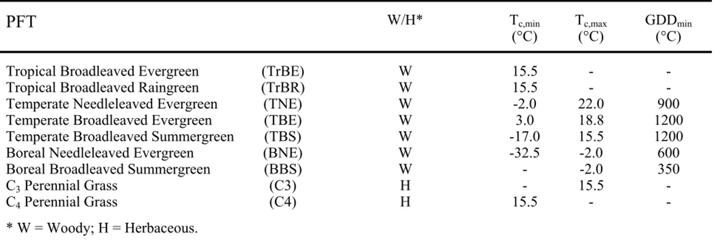
Crucial for the development of DGVMs is the definition of an appropriate set of PFTs. PFTs must be few in number so that they can be parameterized in the global model, but sufficiently complex to cover at least a part of the variety in functional behavior among plants around the globe. For each PFT we need to parameterize the physiological processes. Some PFTs are defined directly on the basis of physiology, e.g. C3 and C4 plants, which by their different photosynthetic pathways respond in different ways to climate change. Other PFT distinctions are made according to leaf longevity, such as between deciduous and evergreen plants.

Dynamic Global Vegetation Models (DGVM), using a given number of PFT, describes the carbon and water exchange between land surface and atmosphere by means of a given set of parameters and input variables. They uses spatially referenced information on climate, elevation, soils and vegetation as well as soil and vegetation specific parameters to make estimates of water and carbon fluxes and pool sizes of terrestrial ecosystems.

A comparison of model results with field data for the location where water and carbon fluxes has been measured provides one reality check. At these sites, measurements of NEP over several years spanning a range of weather conditions provides a measure of how that ecosystem responds to variation in climate. This allows a test of the model’s ability to capture the effects of ecosystem structure and climate on NEP.

2.4 The concept of data assimilation 19

2.4

THE CONCEPT OF DATA ASSIMILATION

Numerical models offer a description of the physical and ecological dynamics of the system of interest at the required time and space scales. However, models are and will always be only a simplified representation of reality. They include a number of approximations, assumptions and uncertainties that cause the model to drift away from the real state of the system that it is designed to predict. Moreover, and this is principally the case with ecological models, with the increasing complexity of the models, also their calibration becomes more and more difficult, due to the increasing number of system parameters. Finally, one of the fundamental insights in physics of the last century was that nature is not deterministic, i.e. even if the current state of a natural system would be fully known, its future state is not uniquely defined. Therefore approaches are needed, that take probabilistic considerations into account, e.g. instead of determining a theoretical future state, give rather an estimation of the most likely realisation of future events, along with its probability and an estimation of the eventual error [Evensen, 2006]. One long term interest of biogeochemical modellers is to first check relatively simple models for consistency and thereby discover the most important processes that need to be considered for large–scale predictions of biogeochemical fluxes. If these most prevailing processes are recovered and correctly parameterised, such a basic model could then be gradually modified and be extended for local process studies as well.

For ecosystem modeling it is inevitable to validate the applied model equations and to justify the associated complexity. Many terrestrial ecosystem models consist of parameterisations which are believed to describe certain biogeochemical processes within the land surface. Only few parameterisations are based upon measurements, conducted in laboratories or only in few different biomes. This is in strong contrast, for example, to physical models of the atmosphere and ocean circulation, which are mainly build on the sound theory of the Navier-Stokes equation. As a consequence, it becomes necessary to study the discrepancies between model results and observations with great care. Such investigations can be subject to three major questions:

1) Are the model’s equations and their spatial discretization appropriate? 2) Are the model’s parameter values optimally chosen?

3) Are the model’s derived variables comparable with in situ observations?

In practice all the questions above cannot be handled separately, making a systematic approach more troublesome. For example, it is difficult to distinguish between the errors which are related

2.4 The concept of data assimilation 20

with the model equations and those which are due to the improper choice of parameter values. If one seeks for the most appropriate prognostic equations or model resolution one must answer, or at least discuss, the second and third question in advance.

With respect to the second question, data assimilation techniques are generally used to find an optimal combination of parameter values that minimise a function which describes the misfits between observation and model results, mostly named objective or cost function (J, Figure 2.5). In other words, data assimilation is a methodology which can optimise the extraction of reliable information from observations and combine it with numerical models.

Figure 2.5. Example of data assimilation in a numerical forecasting system. Considering the observations as a long time sequence of carbon fluxes measured in a given station, we can validate a model output (previous forecast curve) with these measurements. If the model drift away from observations we can “correct” the simulations by data assimilation techniques; in other word we constrain some model parameters in order to minimize the difference between the

model simulation (corrected forecast) and observations.

Thanks to the achievements in research and technology, measurements have become available for a lot of areas of the world and quite efficient and more and more accurate. Considerable effort has been spent to extend and refine the networks of data acquisition and to collect the measurement (e. g. Euroflux, Fluxnet). In particular the use of eddy covariance data has largely increased the availability of essential observational data for TEM, such as water, carbon fluxes and heat fluxes.

2.4 The concept of data assimilation 21

From a methodological point of view, we should use observed carbon and water fluxes at ecosystem scale by the eddy covariance technique to constrain the parameters derived at fine scale in the laboratory or field. This would lead to a parameterization of a global TEM which is adequate for the scale of interest. However, the analysis of parameters and their uncertainties stratified for vegetation type or climate indices allows advanced ecological interpretations, too. The third question deals with the interpretation of biogeochemical measurements and the associated terminology. For the optimisation one usually presumes that the model counterparts to the observations are correctly calculated. In some cases it is still discussed whether a certain measurement, or its procedure, represents a specifically defined biogeochemical process sufficiently well or not. In contrast, the model’s counterparts to the observations are mathematically clearly defined. Consequently, the inconsistency between a model output and a measurement result must not automatically imply that the model equations are wrong but could be subject to the inadequacy of comparing the model’s diagnostic result with the measurement.

III

A

BAYESIAN

INVERSION

OF

LPJ

DYNAMIC

GLOBAL

VEGETATION

MODEL

3.1

INTRODUCTION

The terrestrial biosphere, through biophysical interaction and biogeochemical exchange with atmosphere and ocean, is able to modify local and global climate [Foley et al., 1994; Prentice et

al., 2000].For this purpose, terrestrial ecosystem models have been used extensively to study the processes leading to either carbon loss or gain by the land ecosystem [McGuire et al., 2001;

Prentice et al., 2001].

One important question that models of the carbon cycle could answer is what the future atmospheric concentrations of CO2 may be. The estimates of the terrestrial carbon budget are however highly uncertain [Friedlingstein et al., 2006]. Uncertainties in the model simulations originate both from missing or non-adequate process representation, and from uncertainties in the parameters used. In fact, to run these models, a large number of parameters must be specified. To assign values to the biological parameters is especially difficult, because, unlike many physical or chemical parameters, they cannot be directly measured or regarded as constants [Matear, 1995].

So far, parameters for description of processes like photosynthesis or respiration have been estimated in laboratories or at spatial scales of centimetres to meters in the field [Farquhar et al., 1980; Lloyd and Taylor, 1994]. In global models like TEMs, however, the same equations and most often also the same parameters have been applied to grid cells of 0.5° width and more,

3.1 Introduction 23

which comprise even more than one ecosystem. The reliability of such technique is highly questionable especially because equations are most often derived empirically.

From a methodological point of view, we should use observed carbon and water fluxes at ecosystem scale by the eddy covariance technique to constrain the parameters derived at fine scale in the laboratory or field. In fact, the existence of both a model able to predict the time evolution of one or more variables and of systematic observations leads to an inverse problem; in other words, we can compute few model parameter values in an optimal way, so that the predictions of the model at the stations of measurement in the whole period of observation differ as little as possible from the observations collected.

Recently, the remarkable growing amount of eddy covariance measurements available have allowed to try to quantify uncertainty ranges for some ecosystem model parameters [Knorr, 2000; White et al., 2000; Wang et al., 2001; Reichstein et al., 2003; Braswell et al., 2005; Knorr

and Kattge, 2005; Sacks et al., 2006; Santaren et al., 2007; Wang et al., 2001]. However, eddy

covariance observations have been underutilized in data assimilation studies; only few multi-site assimilation using eddy covariance data has been attempted [e.g. Wang et al, 2007] and for our knowledge no published papers describe the spatial and temporal parameters variability between different ecosystems. Assimilating observations from different eddy covariance sites will reveal how coherent these parameters are both between and within PFTs. Such an analysis will also reveal whether key processes are missing or misrepresented by examining the models’ ability to reproduce observed water and carbon fluxes across a range of spatial and temporal timescales. Various techniques are used for the data assimilation, such as conjugate gradient methods, Kalman Filtering, optimal interpolation (OI), successive corrections and so on [Press et al., 1992]. However, most of these techniques are designed for linear dynamics, and may fail to work correctly in the nonlinear case [Gauthier, 1992; Miller et al., 1994]. Moreover, since our data have errors and the truth is imperfectly known, the problem should be considered as a probabilistic one. That is, the correct solution is not a unique set of parameters but rather a set of parameter estimates along with confidence intervals.

Standard variational methods do not naturally produce this probabilistic information; instead, they merely generate the optimum parameter values. They also require significant effort to implement. In contrast, the Monte Carlo Markov Chain (MCMC) method, based on the Metropolis-Hastings algorithm [Metropolis et al., 1953], is simple to implement, very flexible (including the ability to handle nonlinear models) and produces an ensemble of parameter estimates from which statistical properties can readily be derived and probabilistic forecasts made. The substantial handicap of this method is the massive computational demand which it imposes [Hargreaves and Annan, 2002].

3.2.1 Optimization algorithms 24

3.2

METHODS AND DATA: AN IMPLEMENTATION OF A DATA

ASSIMILATION SYSTEM INTO LPJ

3.2.1 Optimization algorithms

In the present thesis, we developed two different algorithms into LPJ to reduce the mismatch between observations and simulations; each algorithm works minimizing a given cost function (J). The first one (conjugate gradient methods) is a very efficient and fast optimization algorithm that approaches the minimum often within a few iterations. However, when the cost function is a complex surface this algorithm has a tendency to terminate in a local minimum: the failures are attributed to the complex shape of the cost function, caused by non-linearities in the model which lead to discontinuities in the cost function [Matear, 1995]. For such reason there exists an uncertainty in using suitable starting conditions that make it difficult to judge if the global minimum was reached [Aster et al., 2005]. One of the solutions to that problem is to repeat the optimization with various starting points and monitor if they all converge to the same solution [Mary et al., 1998]. However, with the increase in model dimensions the gradient methods is prone to finding a local minimum closest to the starting point rather than the desired global minimum and it is, therefore, the method of choice only for optimizations of low number of parameters [Aster et al., 2005].

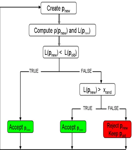
To identify the global minimum, an exhaustive global search method that visits the entire model space using a random walk techniques based on Monte Carlo search have been developed.

This method take advantage of the fact that all local likelihood maxima are sampled if a sufficient number of iterations are performed; for such reason, this method avoid entrapment in local minima and is therefore ideally suited for highly non-linear optimization problems [Mosegaard and Tarantola, 1995]. Each optimization step is only dependent on the previous. The most efficient Monte Carlo method to sample the model space is the Metropolis algorithm [Metropolis et al., 1953]. The Metropolis algorithm performs a random walk (comparable to a Brownian motion) in the model space. The walk is guided by probabilistic rules that decide if a move is accepted or rejected: moves that improve the fit are always accepted, while moves that degrade the fit are accepted with a certain probability. This allows the algorithm to move in and out of local minima.

An advantage of the Monte Carlo search with respect to gradient methods is that it is independent of the structure and analytical properties of the cost function and only requires the evaluation of the cost function. Also, the method is independent of the initial guess because the algorithm enforces a randomization of the initial guess. The major disadvantage is that the

3.2.1 Optimization algorithms 25

stochastic nature of the algorithm requires a large amount of computer time to reach an acceptable final state. The factor controlling the numerical demands of MCMC are the complexity of the model which was integrated may thousand of times, and the number of parameters to optimize.

In the next section, will we described the two different methods from a mathematical point of view. Following Mosegaard and Tarantola [1995], henceforth it is convenient to adopt the subsequent notation:

¾ s denotes the single station where observation are collected.

¾ t is the time (it assumes discrete values since there is a finite sampling time step).

¾ p is the vector of parameters necessary within the model to make predictions.

¾ M(p, s, t) is the prediction of the model, given a certain p, at station s at time t.

¾ D(s, t) is the single observation taken at station s at time t.

In the following D and M(p) and p will be used as vectors.

3.2.1.1 CONJUGATE GRADIENT METHODS

The aim of an inverse algorithm is to find a global minimum of a cost function J(p) in the multidimensional p-space; in other words, we try to reduce the time-space misfits between the observed data D and modeled variables M(p), with the constraints of the model equations and their parameters p. In the Bayesian context, the cost function is usually the sum of two terms: the first term weights the uncertainties of the initial parameters with their respective a priori error covariances. The second term is the sum over time of all data-model misfits at observation locations, weighted by measurement error covariances. Generally, we can write the cost function as: 1 1 0 0 0 1 1 ( ) [ ] [ ] [ ( ) ] [ ( ) ] 2 2 T D J p = p p C− − p p− + M p −D C− M p −DT (3.1)

Here the upper index T indicates matrix transposition, p0 is the vector of a priori guesses for the parameters to optimize, C0 is the diagonal matrix of squared errors that we associate to the a priori guesses, and CD is the diagonal matrix of the squared errors that we associate to the observations.

3.2.1.1 Conjugate gradient methods 26

The solution is sought iteratively by performing several evaluations of the cost function and of its gradient according to:

0

J

∇_p = (3.2)

Descent methods iteratively determine the descending directions along the cost function surface. The minimization can be stopped by limiting the number of iterations, or by requiring that the norm of the gradient ∇ p decreases by a predefined amount during the minimization: this J( ) value is an intrinsic measure of how much the analysis is closer to the optimum.

We employ two different methods to minimize the cost function: 1st derivative (or gradient) of

J(p) to model parameters p ⎛ ∂_{⎜ ∂}J( )

⎝ ⎠

p p

⎞

⎟ yields direction of steepest descent. The method of steepest

descent approaches the minimum in a zigzag manner, where the new search direction is orthogonal to the previous (Figure 3.).

Figure 3.1. Successive minimizations along coordinate directions in a long, narrow “valley” (shown as contour lines). The step size gets smaller and smaller, crossing and recrossing the

valley (from Press et al. [1992]).

The search starts at an arbitrary point X0 and then slide down the gradient, until we are close enough to the solution. In other words, iteration continues until the extreme has been determined with a chosen accuracy ε.

3.2.1.1 Conjugate gradient methods 27

Unless the valley is optimally oriented, this method is extremely inefficient, taking many tiny steps to get to the minimum, crossing and re-crossing the principal axis (Figure 3.) [Press et al., 1992].

2nd derivative (or Hessian) of J (p)

2 2 ( ) ( ) J ⎛ ∂ ⎜ ∂ ⎝ ⎠ ⎞ ⎟ p

p yields curvature of J. The product of the Hessian by the local gradient yields a vector that directly points toward the minimum, even if this vector is oblique with respect to the direction of the steepest descent.

It is easy to see that the gradient (or Newton) methods correspond to obtaining at the current point pi the “paraboloid” that is tangent to the function J(p) and that has the same local curvature and jumping to the point where this tangent paraboloid reaches its minimum [Tarantola, 2005]. Gradient-based methods try to find a compromise between two somewhat contradictory pieces of information. By definition, a gradient-based method uses local information on the function to be optimized, i.e., information that makes full sense in a small vicinity of the current point but does not necessarily reflect the properties of the function in a large domain. But each iteration of a gradient-based method tries to make a jump as large as possible, in order to accelerate convergence. For the intended finite jumps, the local information brought by the gradient may be far from optimal. In most practical applications, the user of a gradient-based method may use physical insight to ‘correct’ the gradient, in order to define a direction that is much better for a finite jump [Tarantola, 2005].

Choosing the right method to be used in an inverse problem is totally problem dependent, and it is very difficult to give any suggestion at the general level. For small-sized problems, Newton methods are easy to implement and rapid to converge. For really large-sized problems, the linear system that has to be solved in the Newton method may be prohibitively expensive and sometimes the methods may not work well [Tarantola, 2005].

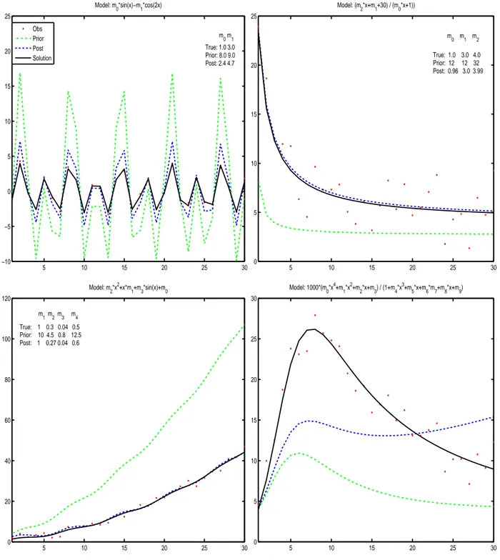
Just to test the performances of the gradient methods a toy model has been developed; a toy model is a simplified set of objects and equations relating them that can nevertheless be used to understand a mechanism that is also useful in the full non-simplified theory.

The complexity of the equations built in the toy model handles both linear and non-linear systems, while the number of parameter to optimize have been changed from few parameters to a huge number according to the LPJ model complexity. In the toy model each number of parameters has associated a given equation (i.e. model, where y=f(x)). The data have been created as follow: once the number of parameters to optimize has been chosen we initialized the

true parameter values to create the model solution, while the observation have been computed

adding a Gaussian noise to the model solution values. The prior (initial) model estimates have been created using guess parameter values (different from true values). Once both observations