Efficiency and instabilities
of financial markets
Lucio Maria Calcagnile
relatori
Prof. Stefano Marmi
Prof. Fulvio Corsi
Tesi di Perfezionamento
Efficiency and instabilities
of financial markets
Lucio Maria Calcagnile
relatori
Prof. Stefano Marmi
Prof. Fulvio Corsi
Tesi di Perfezionamento
in Matematica per le tecnologie industriali
Preface
This thesis tracks my research path, which started right after my master’s de-gree in mathematics, then developed in the 3-year period in which I attended the Perfezionamento in Matematica per le tecnologie industriali at the Scuola Normale Superiore (January 2009–December 2011) and in the subsequent years (2012–present), within the stimulating and original research context created by the collaboration between the mathematical finance group of the SNS and LIST1.2 This collaboration was agreed in November 2011 with the signing of a convention between the two parts, for a 36-month period (later extended) starting from January 2012. The collaboration was signed with the stated primary goals of cooperating in doing research work in common interest areas, which were mainly—but not limited to—quantitative finance, and the exchange of knowledge, both of technical and scientific nature, and of academic and industrial interest. The SNS-LIST collaboration developed within a quantitative finance research laboratory, named QuantLab3, created by LIST within its Advanced Technology Direction. It is in this context that I continued my research path, initially with a 12-month research associate position4 at SNS funded by LIST within the signed convention (January 2012–January 2013), then being directly employed by LIST as quantitative analyst to continue working on the QuantLab activities (May 2013–present). Retracing my research activity from the beginning, in 2010 my first work—made with my two master’s thesis advisors Stefano Galatolo and Giu-lia Menconi—was published on the Journal of Nonlinear Science. It was an
1LIST S.p.A. (member of List Group) is a company developing innovative software
solutions for the financial industry, with its headquarters situated in Pisa. Web site: www.list-group.com.
2In May 2011, the SNS organised the workshop L’instabilit`a nei mercati finanziari: il
Flash Crash un anno dopofor a review of the scientific literature inspired by 6thMay 2010
Flash Crash. It was during this workshop that LIST and the mathematical finance group of the SNS found out the mutual interest in the subject of market instabilities and talked about a possible collaboration to do research on this topic together.
3Web site: www.quantlab.it. 4Assegno di ricerca.
PREFACE
evolution of my master’s thesis work and it was finally printed during the second year of my Perfezionamento course. In this work we studied the entropy—viewed as an ergodic theory concept—of different classes of dy-namical systems, using an information theory approach.
During my Perfezionamento course, first under the guidance of my ad-visor Stefano Marmi and then with the joint mentoring of S. M. and Fulvio Corsi, the idea was born to employ the Shannon entropy as a tool to quan-tify randomness in high frequency financial time series, i.e., as a means to study market informational efficiency analysing high resolution market data. There was some literature about using information theory tools to study market efficiency, but the majority dealt with low frequency (daily) data and those few works actually using high frequency data suffered—from our viewpoint—from serious shortcomings. We took on this problem with a com-bined theoretical and empirical approach, which allowed me to learn a lot of quantitative finance topics and to study in depth the pecularities of high frequency time series, from the stylised facts of intraday price data to many different mathematical approaches used to model them, and to the deep and subtle market microstructure issues. This study was particularly important for my scientific education, because it represented the bridge from genuine mathematics and the fascinating world of quantitative finance.
Thanks to this study on market efficiency with high frequency financial data, I was able to start building a valuable expertise made up both of theoretical knowledge and practical competences, which was very useful in my subsequent work within the SNS-LIST collaboration. Doing research in QuantLab provided me with the double opportunity, on one side, to make the most of the acquired knowledge and, on the other side, to widely deepen it.
The main topic of the research developed in QuantLab was that of finan-cial market systemic instabilities, which revealed to be a fertile research area and—to me personally—a very interesting and stimulating one. The second part of this thesis is made up of two articles written in this context.
The development of the research activity in QuantLab needed a consider-able effort by the involved partners, requiring the engagement of people, the transmission of knowledge between people with different backgrounds, the building of new competences, the designing and realisation of the necessary technological structures. All this was at its very beginning as I was finishing my 3-year Perfezionamento course, so that the research in the QuantLab context could be carried out only in the subsequent years.
I acknowledge LIST for the funding of the research associate position I had at the Scuola Normale Superiore to collaborate in the research project
PREFACE
Metriche di instabilit`a sistemica dei mercati. I also acknowledge the sup-port of the research grant GR12CALCAG Entropia di Shannon ed efficienza informativa dei mercati finanziari at the Scuola Normale Superiore.
Throughout my long research path, I have had the privilege to work with people who have taught me a lot from a scientific point of view and also with whom I have spent many enjoyable moments. I am much obliged to my advi-sor Stefano Marmi, for his wise guidance throughout my long and composite research path. I am also grateful to my advisor Fulvio Corsi, for his precise and valuable help. I am thankful to Fabrizio Lillo, for his valuable guid-ance in a research area where I had a lot to learn. I warmly thank Giacomo Bormetti, for the considerable amount of time we spent working together, for his kind encouragement and for the many enjoyable daily moments we shared.
Finally, I want to thank my parents, who, in their own way, kept en-couraging me in difficult moments of my life. This thesis is dedicated to them.
Lucio Maria Calcagnile
Abstract
In this thesis, we consider two topics in the field of high frequency financial econometrics. The first one is the measurement of market efficiency from high frequency data, within an information theory framework. The study of this topic is performed with an analytical and empirical combined ap-proach. The second topic is that of financial market systemic instabilities at high frequency level and is analysed mainly with an empirical and modelling approach.
In the first part of the thesis, we deal with the question of how market ef-ficiency can be measured from high frequency data. Our interest is motivated on one hand by the availability of high resolution data, that are an incredibly rich information source about financial markets, and on the other hand by some literature on the problem of efficiency measurement that suffers, in our opinion, from serious methodological shortcomings. The process of incorpo-rating the available information into prices does not occur instantaneously in real markets. This gives rise to small inefficiencies, that are more present at the intraday level (high frequency) than at the daily level (low frequency).
Analysing 1-minute and 5-minute price time series of 55 exchange traded funds (ETFs) traded at the New York Stock Exchange (NYSE), we develop a methodology to isolate true inefficiencies from other sources of regularities, such as the intraday pattern, the volatility clustering and the microstructure effects. Our tool to measure efficiency is the Shannon entropy. Since it applies to finite-alphabet symbolic sources, we work with 2-symbol and 3-symbol discretisations of the data.
In the 2-symbol discretisation, one symbol stands for the positive returns, the other for the negative returns. The zero returns, corresponding to price stationarity between consecutive records, are simply discarded. In the 2-symbol discretisation, the intraday pattern and the volatility have no effect, since they are modelled as multiplicative factors. Only the microstructure effects affect the symbolisation. In a first analysis, we test the null
hypoth-ABSTRACT
esis of the symbolised data being indistinguishable from white noise, i.e., uncorrelated data with maximum uncertainty and Shannon entropy equal to 1. Results show, as expected, that the hypothesis is not realistic and that perfect efficiency is rejected in almost all cases. The entropy measurements, however, provide us with a quantification of inefficiency. Data sampled at the frequency of 5 minutes show a higher level of efficiency than those at the 1 minute frequency, confirming that the microstructure effects are greater at higher frequencies.
Market microstructure gives rise to linear autocorrelation that have been modelled in the literature as autoregressive moving average (ARMA) pro-cesses. This motivates us to conduct an analytical study of the Shannon entropy of these processes. We find analytical expressions for the Shannon entropy of order two and three of the AR(1) and MA(1) cases. We also prove a number of results about general properties of the probabilities of fi-nite binary sequences derived from the AR(1) and MA(1) processes, that are applicable and useful to obtain (at least partial) results about the entropies of order greater than three. All this analytical work and the results about the AR(1) and MA(1) Shannon entropy are original and we dedicate a sep-arate chapter to this subject. We believe that these results and the whole approach have their own interest and can be useful in other contexts as well. Relying on the ARMA modelling of asset returns, we follow two ways. For the series that are best fitted with an AR(1), an MA(1) or a simple white noise process, we define a measure of inefficiency as the (suitably normalised) difference between the Shannon entropy measured on the data and the the-oretical value of the Shannon entropy of the corresponding process. For the other series, which are best fitted with ARMA(p, q) models with p + q > 1, we define a measure of inefficiency as the (suitably normalised) difference between 1 (the entropy of a white noise process) and the Shannon entropy of the ARMA residuals. Results show that in some cases a large part of the ap-parent inefficiency is explained by the linear dependence structure, while in many other cases the ARMA residuals continue to contain some (nonlinear) inefficiencies. We also rank the ETFs according to the measured inefficiency and notice that the rankings are not very sensitive to the choice of the en-tropy order. By rigorously testing the ARMA residuals for efficiency, we reject the hypothesis of efficiency for the large majority of the ETFs.
We find a strong relationship between low entropy and high relative tick size. This is explained by noting that an asset’s price with a large relative tick size is subject to more predictable changes. We also notice an interesting relation between the inefficiency of ETFs tracking the indices of countries, with the ETFs of the Asian/Oceanic countries being very inefficient, the ETFs tracking the indices of European countries showing a moderate amount
ABSTRACT
of inefficiency and ETFs relative to American countries being among the most efficient. The levels of detected inefficiency for the country ETFs can be related to the opening time overlap between the country markets and the NYSE, where the ETFs are exchanged with a trading dynamics that can or cannot rely on a simultaneous evolution of the corresponding indices. We hypothesise that those ETFs that track indices of markets that are closed during the ETFs’ trading time are deliberately given a low price, since their dynamics is only coarsely determined.
In a 3-symbol discretisation, one symbol represents a stability basin, en-coding all returns in a neighbourhood of zero. Negative and positive returns lying outside of this basin are encoded with the other two symbols. Previous works working with a 3-symbol discretisation of data fix absolute thresholds to define this basin. We argue that there are numerous problems in doing so and, as a major enhancement with respect to such literature, we propose a very flexible approach to the 3-symbol discretisation, which is also rather general. We define the thresholds for the symbolisation to be the two ter-tiles of the distribution of values taken by the time series. Such a definition has many advantages, since, unlike a fixed-threshold symbolisation scheme, it adapts to the distribution of the time series. This is important because different assets have different distributions of returns and fixed thresholds could introduce discrepancies in treating the different time series. Moreover, the distribution of returns also varies with the sampling frequency, so that a fixed symbolisation scheme for different frequencies appears inappropriate. Finally, our flexible tertile symbolisation can be applied not only to the raw return series, but also to series of processed returns whose values range on different scales. Such are the cases of the returns filtered for the intraday pattern, of the volatility-standardised returns and of the ARMA residuals.
Using the tertile symbolisation, we investigate to what degree the intraday pattern, the volatility and the microstructure contribute to create regulari-ties in the return time series. We follow a whitening procedure, starting from the price returns, removing the intraday pattern, thus getting the deseason-alised returns, then standardising them by the volatility, finally filtering the standardised returns for the ARMA structure and getting the ARMA resid-uals. We symbolise all these series with the dynamic tertile thresholds and estimate the Shannon entropy of the symbolis series to measure their degree of randomness.
Results show that, in the vast majority of cases, the raw return symbolised series are the most predictable, with the removal of the intraday component making the series more efficient. The most noteworthy results come however from the standardisation step. The removal of the volatility is responsible for the largest increase in the entropy, meaning that volatility gives the return
ABSTRACT
series a huge amount of regularity. On average, this effect is larger (62%) than the combined effect of the intraday (18%) and microstructure (20%) regularity. This result convincingly demonstrates that, when studying the randomness of a three-symbol discretised time series, the volatility must be filtered out. Omitting this operation would give results that tell more on the predictable character of the volatility than on, for example, market effi-ciency. The last whitening step, consisting in removing the ARMA structure, further contributes to move return series towards perfect efficiency. Overall, our results show that much of the assets’ apparent inefficiency (that is, the predictability of the raw return series) is due to three factors: the daily seasonality, the volatility and the microstructure effects.
In the second part of the thesis we deal with the topic of abnormal high frequency returns of asset prices5 and systemic instabilities of financial mar-kets. We also develop two different modelling approaches. Modelling the dynamics of large movements in security prices is of paramount importance for risk control, derivative pricing, trading and to understand the behaviour of markets. Our interest for the topic is motivated by the importance of understanding the consequences that the increase of algorithmic and high frequency trading has on market stability, in a context of more and more in-terconnected markets, where technological progress has deeply changed both the way that trading is performed and the velocity of the spread of informa-tion.
The purpose of this research is a deep understanding of the dynamics of market instabilities, from many different viewpoints, with particular interest in systemic events. We devote our attention to the study of their statisti-cal properties, their historistatisti-cal evolution, their relation with macroeconomic news, their autocorrelation and dependence properties, their modelling.
We identify the intraday times of abnormal returns by means of a jump identification procedure based on the standardisation of one minute returns by the intraday pattern and the local volatility. In a first work (Chapter 8), we show that the dynamics of jumps of a portfolio of stocks deviates signif-icantly from a collection of independent Poisson processes. The deviation that we observe is twofold. On one side, by considering individual assets, we find evidence of time clustering of jumps, clearly inconsistent with a Poisson process. This means that the intensity of the point process describing jumps depends on the past history of jumps and that a recent jump increases the probability that another jump occurs. The second deviation from the
Pois-5We refer to abnormal returns of asset prices also as jumps or instabilities.
ABSTRACT
son model is even more relevant, especially in a systemic context. We find a strong evidence of a high level of synchronisation between the jumping times of a portfolio of stocks. In other words, we find a large number of instances where several stocks jump within the same one minute interval (which is our maximum resolution). This evidence is absolutely incompatible with the hypothesis of independence of the jump processes across assets.
In order to model the time clustering of jumps for individual assets we propose the use of Hawkes processes, a class of self-exciting point processes, which reveal to be very effective in describing the single asset jumping proper-ties. However, the natural extension of the application of Hawkes processes to describe the dynamics of jumps in a multi-asset framework, i.e., considering multivariate Hawkes processes, is highly problematic due to the exponential growth of the parameter number and, more importantly, it is inconsistent with data. In fact, even considering just two stocks, we find that a bivariate Hawkes model is unable to describe the high number of synchronous jumps that we empirically observe in the data. This is due to the fact that the kernel structure of Hawkes is more suited to model lagged jumps rather than synchronous jumps. Our main contribution is the introduction of a Hawkes factor model to describe systemic events. We postulate the presence of an unobservable Hawkes process describing a market jump factor. When this factor jump, each asset jumps with a given probability, which is different for each stock. An asset can jump also by following an idiosyncratic Hawkes process. We show how to estimate this model and how to discriminate be-tween systemic and idiosyncratic jumps. Results from simulations of the model show that it is able to reproduce the main features that characterise the departure from a random behaviour of jumps, namely, the time cluster-ing of jumps on individual stocks, the large number of simultaneous systemic jumps and the time lagged cross-excitation between different stocks.
In a second work (Chapter 9), we analyse one-minute data of 140 stocks for each year from 2001 to 2013, addressing other questions. Concerning the evolution of the dynamics of market instabilities in the last years, our research provides the empirical evidence that, while the total number of extreme price movements has decreased along the years, the occurrence of systemic events has significantly increased. This trend is more and more pronounced when considering events of higher and higher level of systemicity. To identify the possible causes of such events we compare their time occurrences with a database of pre-scheduled macroeconomic announcements, which can be ex-pected to have a market-level influence and to possibly explain market-wide events. Unexpectedly, only a minor fraction (less than 40%) of events in-volving a large fraction of assets has been preceded by the release of a macro news. This evidence leaves room for the hypothesis that financial markets
ABSTRACT
exhibit systemic instabilities due to some endogenous dynamics, resulting from unstable market conditions such as a temporary lack of liquidity.
Finally, we provide the evidence that highly systemic instabilities have the double effect of (i) increasing the probability that another systemic event takes place in the near future and (ii) increasing the degree of systemicity of short-term instabilities. In order to reproduce such empirical evidences, we propose a model within the class of multivariate Hawkes processes, with mu-tually exciting properties. We present a multidimensional—yet parsimonious in the number of parameters—Hawkes process which provides a realistic de-scription of the market behaviour around systemic instability events.
Chapter 2 has a mathematical character and introduces the concepts of information source and entropy in the context of dynamical systems and random processes.
Chapter 3 presents and compares some methods to estimate the entropy of dynamical systems, with a combined ergodic theory and information theory approach. It is constituted by the publication (P1).
In Chapter 4 we develop the analytical study of the entropy of the AR(1) and MA(1) processes, motivated by the study on market efficiency of Chapter 7. This is original content and constitutes part of the preprint (P4).
In Chapter 5 we review the application of information theory to gam-bling and portfolio theory developed by Kelly. The presentation follows [1]. We also review the Efficient Market Hypothesis and some literature on the measuring of market efficiency from real data.
In Chapter 6 we present the stylised facts of high frequency financial data and the data cleaning procedures that we use to filter them out in the analyses of Chapters 7, 8 and 9.
In Chapter 7 we develop our study of market efficiency measurement using the Shannon entropy. We use both an analytical approach, using the theoretical results obtained in Chapter 4, and a more empirical one. The content of this chapter is original and constitutes—together with Chapter 4—the preprint (P4).
Chapter 8 contains our first work on market instabilities. It focuses on methods for their detection and on the development of the Hawkes models
ABSTRACT
for their modelling. This chapter also constitutes the publication (P2).
Chapter 9 is our second work on market instabilities, treating the topics of the historical evolution of instabilities, their exogenous/endogenous origin, the analyses about the systemicity levels and their modelling. It constitutes the preprint (P3).
List of publications
(P1) L. M. Calcagnile, S. Galatolo, G. Menconi, Non-sequential Recursive Pair Substitutions and Numerical Entropy Estimates in Symbolic Dy-namical Systems, Journal of Nonlinear Science, 20 (2010), pp. 723–745
(P2) G. Bormetti, L. M. Calcagnile, M. Treccani, F. Corsi, S. Marmi, F. Lillo, Modelling systemic price cojumps with Hawkes factor models, Quanti-tative Finance 2015, DOI: 10.1080/14697688.2014.996586
(P3) L. M. Calcagnile, G. Bormetti, M. Treccani, S. Marmi, F. Lillo, Collec-tive synchronization and high frequency systemic instabilities in finan-cial markets; preprint at http://arxiv.org/abs/1505.00704
(P4) L. M. Calcagnile, F. Corsi, S. Marmi, Entropy and efficiency of the ETF market ; preprint at http://arxiv.org/abs/1609.04199
Contents
Preface iii
Abstract vii
List of publications xv
1 Introduction 1
1.1 Measuring the informational efficiency of markets with the
Shannon entropy . . . 2
1.2 Studying and modelling the properties of market instabilities . 6
I
Entropic measures of market efficiency
11
2 Information sources and entropy 13 2.1 Introduction . . . 132.2 Information sources . . . 14
2.2.1 Random processes and sequence spaces . . . 14
2.2.2 Shift transformations . . . 16
2.2.3 Dynamical systems . . . 16
2.2.4 From dynamical systems to symbolic dynamics . . . . 19
2.2.5 Ergodicity . . . 20
2.3 Entropy . . . 22
2.3.1 Introduction . . . 22
2.3.2 Entropy of a random process . . . 23
2.3.3 Entropy of a dynamical system . . . 25
3 Estimating entropy from samples 29 3.1 Non-sequential recursive pair substitution . . . 30
3.1.1 Introduction . . . 30
3.1.2 Definitions and results on the NSRPS method . . . 31
CONTENTS
3.2 Empirical frequencies (EF) . . . 35
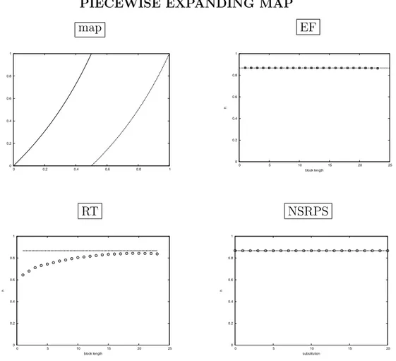
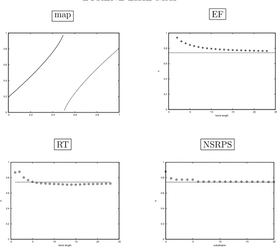
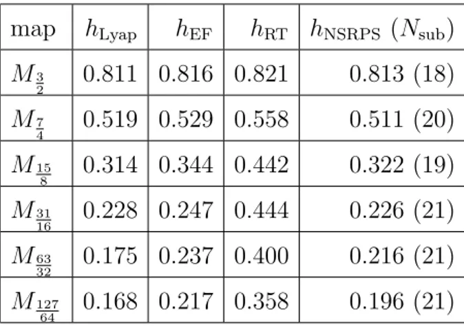
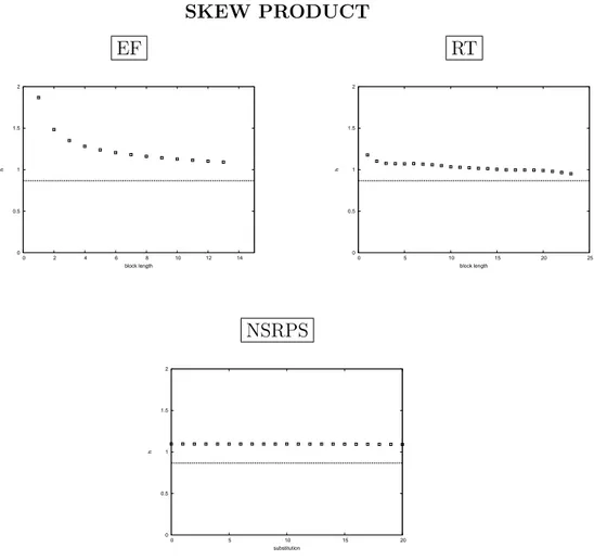
3.3 Return times (RT) . . . 36 3.4 Lyapunov exponent . . . 37 3.5 Computer simulations . . . 38 3.6 Experiments . . . 39 3.6.1 Maps . . . 40 3.6.2 Renewal processes . . . 47 3.7 Conclusions . . . 49
4 Entropy of the AR(1) and MA(1) processes 53 4.1 The AR(1) and MA(1) processes . . . 54
4.1.1 The AR(1) process . . . 54
4.1.2 The MA(1) process . . . 55
4.2 The Shannon entropy of the processes AR(1) and MA(1) . . . 56
4.2.1 A geometric characterisation of the Shannon entropies HkAR(1) . . . 59
4.2.2 Calculating the entropies Hk . . . 61
5 Gambling, portfolio theory and market efficiency 65 5.1 Gambling . . . 65
5.1.1 Dependent horse races and entropy rate . . . 67
5.2 Information theory and portfolio theory . . . 68
5.2.1 Duality between the growth rate and the entropy rate of a market . . . 69
5.3 Market efficiency . . . 71
5.3.1 A brief history . . . 71
5.3.2 The random walk hypothesis . . . 71
5.3.3 Efficient Market Hypothesis: the weak, the semi-strong and the strong form . . . 72
5.3.4 Refutability of the EMH . . . 72
5.3.5 Relative efficiency . . . 73
5.4 Literature review on measuring market efficiency . . . 73
5.4.1 Measuring market efficiency with the Lempel-Ziv com-pression index . . . 74
5.4.2 Measuring market efficiency with a Variable Order Markov model . . . 77
5.4.3 Measuring market efficiency with the Shannon entropy 80 5.4.4 Measuring market efficiency with the Hurst exponent and the Approximate Entropy . . . 81
CONTENTS
6 High frequency data 83
6.1 Stylised facts for intraday returns . . . 83
6.2 Cleaning and whitening . . . 84
6.2.1 Outliers . . . 84
6.2.2 Stock splits . . . 85
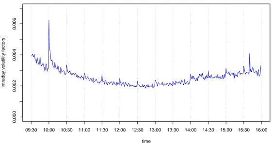
6.2.3 Intraday patterns . . . 85
6.2.4 Heteroskedasticity . . . 86
7 The informational efficiency of financial markets 89 7.1 ETF data . . . 90
7.1.1 Exchange Traded Funds . . . 90
7.1.2 Dataset . . . 91
7.1.3 Data cleaning . . . 91
7.2 Binary alphabet . . . 95
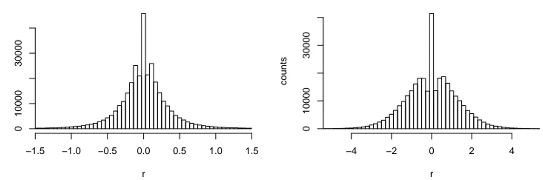
7.2.1 Discretising returns . . . 95
7.2.2 Modelling return series as AR(1) or MA(1) processes . 99 7.2.3 Modelling return series as ARMA(p, q) processes . . . . 102
7.3 Ternary alphabet . . . 111
7.3.1 The impact of intraday patterns and volatility on mar-ket efficiency measures . . . 113
7.4 Conclusions . . . 116
II
Market instabilities
119
8 Modelling systemic price cojumps with Hawkes factor mod-els 121 8.1 Introduction . . . 1218.2 Data description and data handling . . . 125
8.2.1 Intraday pattern . . . 127
8.3 Jump identification . . . 128
8.3.1 Performance of the jump detection methods on simu-lated data . . . 130
8.4 Basic statistics of jumps of individual stocks and of systemic jumps . . . 132
8.4.1 Jumps of individual stocks . . . 132
8.4.2 Systemic jumps . . . 135
8.5 A multi-scale statistical test based on multiple jumps and cross jumps detection . . . 137
8.5.1 A benchmark case: the Poisson model . . . 140
CONTENTS
8.6.1 Univariate case . . . 142 8.6.2 Bivariate case . . . 144 8.7 A factor model approach to systemic jumps . . . 146 8.7.1 Bivariate Poisson factor model . . . 147 8.7.2 N dimensional Hawkes factor model with idiosyncratic
components . . . 148 8.8 Robustness analysis . . . 152 8.9 Conclusions and perspectives . . . 157 8.10 Appendix: Volatility auctions . . . 160
9 Collective synchronization and high frequency systemic in-stabilities in financial markets 161 9.1 Introduction . . . 161 9.2 Data . . . 163 9.2.1 Financial data . . . 163 9.2.2 News data . . . 163 9.3 Methods . . . 164 9.3.1 Identification of extreme events . . . 164 9.4 Results . . . 164 9.4.1 Historical dynamics of jumps and cojumps . . . 165 9.4.2 Systemic cojumps and macroeconomic news . . . 167 9.5 Model . . . 169 9.5.1 Hawkes process for multiplicity vector . . . 169 9.5.2 Model results . . . 170 9.6 Discussion . . . 172 9.7 Appendix A: Data . . . 173 9.7.1 Market data . . . 173 9.7.2 News data . . . 174 9.8 Appendix B: Dependence of systemic cojumps on time scale
detection . . . 174 9.9 Appendix C: Model . . . 175 9.9.1 Multivariate Hawkes point processes . . . 175 9.9.2 Choice of the parametrization . . . 176 9.9.3 Estimation of the model parameters . . . 178 9.9.4 Results for the investigated dataset . . . 179 9.9.5 Model results for the years 2001–2012 . . . 180
Bibliography 189
Chapter 1
Introduction
Central theme of this thesis is the analysis of high frequency financial data. In recent years, the wide availability of high resolution data has renewed and stimulated the interest of researchers with a mathematical and physical background towards the complex world of financial markets.
The mathematical study of financial markets has a long history and a multitude of approaching methods. One that we find particularly fascinating is the attempt to transport to financial markets some concepts from the theory of dynamical systems. For example, in the late 1980s and especially during the 1990s, some literature focused on the concept of chaos in financial markets, i.e., the apparently random behaviour of markets as the result of a nonlinear dynamics. See [2] for a literature review on the topic of chaos in financial markets and [3, 4] for notable works on the subject. There is also a sizeable amount of literature on the concept of entropy in finance, which has been used as an important tool in portfolio selection [5, 6, 7], asset pricing [8, 9, 10, 11], Efficient Market Hypothesis testing and market efficiency measuring [12, 13, 14]. We investigate how entropy can be used to quantify inefficiency, with the awareness that high frequency data, alongside with the advantage of providing a much higher amount of information than low frequency—daily, at most—data, also present serious challenges.
Another topic that, especially in recent years, has attracted the attention of researchers is that of market instabilities. Recent crashes—the biggest and most famous one being the 6th May 2010 Flash Crash—have posed several questions about their nature, e.g., how frequently do they happen?, are they occurring more and more frequently?, are their causes exogenous or endoge-nous to the markets? We study detection techniques, correlation properties, historical evolution, exogenous/endogenous origin, modelling possibilities.
In this thesis, we deal with the two aforementioned topics, namely the problem of measuring the informational efficiency of markets and the study
CHAPTER 1. INTRODUCTION
and modelling of market instabilities, in both cases with high frequency fi-nancial data as our starting point.
1.1
Measuring the informational efficiency of
markets with the Shannon entropy
Financial markets are places where information plays a major role. The agents in the market trade based on all the available information—public and private—and it can also be said that the collective trading activity itself generates new information. It is no surprise that, in this context of hid-den and manifest information, information theory was applied. Information theory has a precise beginning, identifiable in Claude Shannon’s ground-breaking 1948 paper A Mathematical Theory of Communications, published on the Bell System Technical Journal [15]. Though—as acknowledged by Shannon himself in the beginning of his paper—a basis for a general the-ory of communication was contained in the work of Nyquist and Hartley at Bell Laboratories in the 1920s, it was Shannon’s unifying vision that revo-lutionised communication, developing the first key concepts and inspiring a multitude of research topics that we now define as the field of information theory.
In his paper Shannon introduced four major concepts: the channel ca-pacity, i.e., the concept that every communication channel has a speed limit, measured in binary digits per second; the digital representation of data (the term bit is used in his article for the first time), be it text, sound, image or video; the concept of source coding, which deals with efficient represen-tation of data and is now synonymous with data compression, based on the removal of redundancy in the information to make the message smaller; the quantification of the amount of information in a signal, called entropy. The entropy of a source is essentially an average measure of the randomness of its outputs. It represents the average amount of information that the source transmits with each symbol, or, equivalently, the average amount of uncer-tainty removed with the transmission of each symbol.
Soon after Shannon developed the entropy theory of information, many attempts were made to give information a more intuitive meaning and prac-tical applications. In his 1956 paper A New Interpretation of Information Rate [16], Kelly proved that a gambler with side information could use some of Shannon’s equations to achieve the highest possible return on his capital. Presenting his idea as a system for betting on horse races, Kelly showed that the gambler’s optimal policy is to maximise the expected logarithm of wealth
1.1. MEASURING THE INFORMATIONAL EFFICIENCY OF MARKETS WITH THE SHANNON ENTROPY
and that this goal is achieved with the gambling scheme where bets on each horse are proportional to the probability that each horse will win.1 Kelly also showed that the financial value of side information (i.e., the increase in wealth that results from that information) is equal to the mutual informa-tion between the horse race and the side informainforma-tion. The strong connecinforma-tion between information theory and gambling on horse races was also extended to the financial markets in the broader concept of portfolio selection, high-lighting how striking the parallels between the theory of optimal investment in the stock market and information theory are. In fact, gambling on horse races can be viewed as a special case of portfolio selection, since placing bets in a race with m horses corresponds to investing on m special stocks in the market, where the final value of the stock for horse i is either 0 or the value of the odds for horse i. Both in the context of horse races and of a stationary stock market, it has been shown that the growth rate of the wealth is a dual of the entropy rate. The theory of growth optimal portfolios was introduced by Kelly [16] and Latan´e [17] and generalized by Breiman [18]. Barron and Cover [19] proved that the mutual information between some side informa-tion and the stock market is an upper bound on the increase in the growth rate.
A market is said to be informationally efficient if it is efficient in process-ing the information. In an efficient market observed prices express a correct evaluation of all available information. The concept of market efficiency was first anticipated by Bachelier in 1900, who writes in his PhD dissertation that “past, present and even discounted future events are reflected in market price, but often show no apparent relation to price changes.” [20]. Modern literature on market informational efficiency begins however in the 1960s, with the independent works of Samuelson and Fama. The idea that asset prices fully reflect all available information (the so-called Efficient Market Hypothesis (EMH) was introduced in modern economics by Samuelson, with his article [21]: Proof that properly anticipated prices fluctuate randomly. Samuelson observed that “[i]f one could be sure that a price would rise, it would have already risen.” It was Fama, though, the first to introduce the term ‘efficient market’ [22]. In his seminal papers [23, 24, 22, 25] he was con-cerned with the old debate between technical analysis (the use of patterns in historical data to forecast future prices) and fundamental analysis (the use of accounting and economic data to establish the assets’ fair prices).
Fama proposed three forms of the efficient market hypothesis, correspond-ing to different information sets available to market agents. The weak form
1This strategy is called Kelly criterion, Kelly betting, Kelly formula, proportional betting
CHAPTER 1. INTRODUCTION
says that prices fully reflect the information contained in past prices. The semi-strong form maintains that prices fully reflect all publicly available formation. The strong form asserts that market prices fully reflect any in-formation, public and private.
Market efficiency implies the random character of prices (the more effi-cient the market, the more random the sequence of price changes). A per-fectly efficient market is one in which price changes are completely random and unpredictable. This ideal situation is the result of many market par-ticipants attempting to profit from their information. When investors try to exploit even the smallest informational advantages at their disposal, their actions have the effect of incorporating the information into market prices, so that in the end the profit opportunities that first motivated the trades are quickly eliminated.
A statistical description of the unforecastability of price changes is pro-vided by the so-called random walk hypothesis (RWH), suggesting a model in which prices evolve in a purely random manner. Much of the literature about market efficiency revolved around the RWH and testing for the presence of patterns in historical market data. A number of works testing data for the RWH were published from the beginning of the 1960s to the beginning of the 1990s, with general results supporting the RWH for daily data and only occasional results of departure from randomness and rejection of the RWH [26].
Fama [25] summarises the early random walk literature, his own contri-butions and other studies about the information contained in the historical price time series and concludes that the results strongly support the weak form of the EMH. The evidence accumulated in the 1960s and 1970s shows that, while markets cannot be completely efficient in the strong form, there is convincing support for the weak and semi-strong forms. Departures from the EMH are commonly explained as consequences of over- or underreaction to new information by the investors, when prices are temporarily pushed be-yond the fair or rational market value and subsequently adjusted, with the formation of patterns.
As pointed out by Campbell, Lo, MacKinlay [27], perfect informational efficiency is an idealised condition which is never met in real markets. Inef-ficiencies are always present in real markets and there is no point in investi-gating the efficiency of markets in absolute terms. Rather than the absolute view taken by the traditional literature on market efficiency, it is much more interesting to study the notion of relative efficiency, that is, the degree of effi-ciency of a market measured against the benchmark of an idealised perfectly efficient market.
We stress that this is the point of view we take in this work. We shall
1.1. MEASURING THE INFORMATIONAL EFFICIENCY OF MARKETS WITH THE SHANNON ENTROPY
investigate to what degree assets depart from the idealised perfect efficiency, ranking them according to relative efficiency.
Relative efficiency was studied in [28, 29, 30, 13, 31, 12], where different concepts and tools were used to measure the amount of randomness in the historical return time series, namely, the algorithmic complexity, a variable-order Markov model, the Shannon entropy, the Hurst exponent, the approx-imate entropy. All these works have in common the procedure of translating a data time series into a symbolic one, by assigning a symbol to a particular behaviour of the price (for example, symbols 0, 1, 2 are given the meaning of ‘the price goes down’, ‘the price goes up’, ‘the price remains stable’ and the return time series is translated into a sequence of 0s, 1s and 2s). This is also what we do in Chapters 4 and 7, investigating symbolisations of stochastic processes and historical time series into 2 or 3 symbols. Like [13], we use the Shannon entropy as a tool for measuring the randomness of the series.
In [28, 29, 30] the authors measure the relative efficiency of the return time series by means of a 3-symbol discretisation, with one symbol representing the price stability behaviour, defined as the absolute value of price returns— or of price differences, in one case—being less than a threshold. A serious shortcoming of their procedure, however, is that they do not normalise re-turns for the volatility. In our opinion, much of the apparent inefficiency they find in the series is essentially due to the persistency of volatility, which trans-lates into the three symbols forming patterns (in periods of high volatility the two symbols not representing price stability will be very frequent, while the opposite will hold in periods of low volatility).
All the cited papers dealing with relative efficiency, with the exception of [30], deal with daily data. Working instead with high frequency data (i.e., intraday price records) is both very interesting and very challenging. As long as the amount of information is concerned, intraday data obviously provide a much richer source than daily data. Moreover, it is more natural to investigate the presence of recurring patterns and inefficiencies at a high frequency level, since at the daily level they tend to compensate. On the other hand, we have to confront ourselves with new problems. The fact that a security has different buy and sell prices and the fact that prices move on a discrete grid are known as microstructure effects, since they depend on the structure of the market and on the price formation mechanism. They are sources of regularity in recorded price series—they add autocorrelation—and can play a major role especially for low liquidity assets. These effects add spurious regularity to the series, which must be properly discounted if one wants to quantify the true efficiency.
The scientific literature has proposed a variety of approaches to the mod-elling of microstructure. An interesting one is the modmod-elling by means of
CHAPTER 1. INTRODUCTION
the autoregressive–moving-average (ARMA) models. These models are able to capture the return series autocorrelation due to the microstructure fea-tures. The benchmark provided by the ARMA models can be used in two different ways. One way is estimating the best model on the data and taking the time series of residuals2, then analysing the residual time series to quan-tify the remaining regularities. Another way to use the benchmark of the autoregressive moving-average models is to compare the randomness of the data time series with the theoretically calculated value of the randomness of the ARMA models. We follow both approaches, developing an interesting theoretical study about the Shannon entropy of ARMA models.
Our method to measure the assets’ efficiency is designed to discount all known sources of regularity of high frequency data: the intraday pattern, the long-term volatility and the microstructure effect. Only the inefficiency that remains in the processed series, after these effects have been filtered out, can be regarded as the true inefficiency.
1.2
Studying and modelling the properties of
market instabilities
Recent years have seen an unprecedented rise of the role that technology plays in all aspects of human activities. Unavoidably, technology has heavily entered the financial markets, to the extent that all major exchanges are now trading exclusively using electronic platforms. This has profoundly changed the way the trading activity is conducted in the market, from the old phone conversation or click and trade on a screen to software programming. In algo-rithmic trading, computer programs process a large amount of information— from market data to political news and economic announcements—and out-put trading instructions with no human intervention being required. Trading algorithms include the search for arbitrage opportunities (for example, small discrepancies in the exchange rates between three currencies), the search for optimal splitting of large orders at the minimum cost, the implementation of long-term strategies to maximise profits. An important class of algorithms is devoted to the automatic parsing and interpretation of news releases, result-ing in tradresult-ing orders beresult-ing generated before humans have even read the news title. Electronic platforms and new technologies have facilitated the flourish-ing of the so-called high frequency tradflourish-ing, which is nowadays a significant fraction of all the trading activity in US and Europe electronic exchanges
2Residuals can be thought of as the term-by-term difference between the data and the
fitted model.
1.2. STUDYING AND MODELLING THE PROPERTIES OF MARKET INSTABILITIES
[32].
It has been argued that high frequency trading is beneficial to the dis-covery of the efficient price [33]. Arbitrage opportunities that may originate under some circumstances are promptly exploited—and thus eliminated—by algorithms that act as high frequency traders, resulting in a more efficient price. On the other side, the ultra fast speed of information processing, order placement and cancelling potentially allows large price movements to propa-gate very rapidly through different assets and exchanges [34], and is believed to be a means of contagion and the cause of an increased synchronisation among different assets and different markets.
On 6th May 2010, this synchronisation effect had its most spectacular appearance in what is known as the Flash Crash. The crash started from a rapid decline in the E-Mini S&P 500 market and in a very short time the anomaly became systemic and the shock propagated towards ETFs, stock indices and their components, and derivatives [35, 36]. The price of the Dow Jones Industrial Average plunged by 9% in less than 5 minutes but recovered the pre-shock level in the next 15 minutes of trading. The SEC reported that such a swing was sparked by an algorithm executing a sell order placed by a large mutual fund. Then high frequency traders, even though did not ignited the event, caused a “hot potato” effect amplifying the crash. In the aftermath of the crash, several studies have focused on events, evocatively named mini flash crashes, concerned with the emergence of large price movements of an asset in a very limited fraction of time and attributing their origin to the interaction between several automatic algorithms [37] or to the unexpected product of regulation framework and market fragmentation [38].
In recent years, it has been observed a growing tendency of the financial markets to exhibit systemic instabilities, i.e., sudden large price movements involving a great part of the market. Researchers have tried to answer the following questions. Are these extreme price fluctuations driven by the re-lease of price sensitive information? Or, on the contrary, are these events an effect of any unrevealed endogenous dynamics? Many such events can-not be associated with exogenous events such as news releases and it has been suggested in literature that this susceptibility may be generated in an endogenous way by the trading process itself. The Flash Crash has dramat-ically shown how strongly interconnected different markets and asset classes can become, especially during extreme events.
Scientific literature about discontinuities in asset prices has concentrated mostly on the identification problem at the daily time scale, i.e., on trying to answer the question of whether an extreme return occurred on a given day. This topic, referred to as the jump identification problem in the econometric literature, was extensively studied in theoretical works as well as in empirical
CHAPTER 1. INTRODUCTION
analysis and applications to asset pricing. Significantly less research—and mainly of empirical nature—has been devoted to the study of cojumps, i.e., large price movements occurring synchronously in two or more assets. In literature, the modelling of discontinuities in the dynamics of asset prices is commonly performed by means of a compound Poisson process, see e.g. [39]. While having the great advantage of being analytically tractable, Poisson processes (as well as the more general L´evy processes) have independent in-crements and thus cannot account for any kind of serial or cross-sectional correlation. It is instead reasonable to presume that the jump component of the price process has some clustering properties and that a better choice for its modelling would be one that allows some dependence between the jump-ing times. Moreover, considerjump-ing the increased interconnection of electronic markets, it is reasonable to expect some synchronisation between the jump-ing times of different assets. This is particularly important when aimjump-ing to describe and model events of systemic instabilities such as the Flash Crash, for which using independent jump processes would clearly be inadequate.
A class of self-exciting point processes that are good candidates to well describe the correlation properties of the jump time series is that of Hawkes processes. These processes were introduced in seismology more than forty years ago [40] and have been widely employed to model earthquake data [41, 42]. In recent years, Hawkes processes have become popular also in math-ematical finance and econometrics [43, 44, 45]. They have been effectively used to address many different problems in high-frequency finance, such as estimating the volatility from transaction data, devising optimal execution strategies or modelling the dynamics of the order book.
A univariate Hawkes process is a point process whose intensity is the sum of two components: the baseline intensity, responsible for the happening of events unrelated to the history of the process up to the present time, and a backward-looking kernel, which adds a further intensity for every past event (more recent events give a higher contribution) and is responsible for the generation of child events, i.e., events triggered by previous ones. A univari-ate Hawkes process is thus a natural choice for trying to model a clustered time series like the one of an asset price jumps. While the baseline intensity could explain the exogenously generated jumps, the kernel could account for the endogenous mechanisms of self-excitement and auto-triggering.
In a global perspective, considering market instability properties means looking also at cross-asset dependencies and mutual excitement properties. Since in a highly connected market large price movements in one asset can propagate and thus be responsible of extreme returns in other assets, a model describing global instabilities must necessarily possess inter-asset correlations or some kind of multi-asset features.
1.2. STUDYING AND MODELLING THE PROPERTIES OF MARKET INSTABILITIES
It is natural to consider multivariate Hawkes processes, multidimensional point processes which possess, along with the self-exciting properties of stan-dard univariate Hawkes processes, also cross-exciting properties for every possible pair of processes. However, as we show in Chapter 8, they present two notable downsides. Firstly, the number of parameters of a multivari-ate Hawkes process grows quadratically with the dimension, i.e., an N-dimensional Hawkes process has O(N2) parameters, and thus its estimation becomes unfeasible for high dimensions. Secondly, but more importantly, we find that even a 2-dimensional Hawkes model is not able to reproduce the high number of synchronous jumps observed in empirical data. These considerations led us to search for different approaches.
In a first work, Chapter 8, we investigate the one-asset and multiple-asset jump clustering properties. After studying the performance of our jump identification method and analysing some statistical properties of jumps of individual stocks and of systemic jumps, we first compare the empirical data with a Poisson benchmark and then develop the Hawkes modellisation of the jump dynamics. Since, as said before, bivariate Hawkes processes fail at describing the cojump properties of asset pairs, we develop a Hawkes factor model, which postulates the presence of an unobservable point process describing a market factor. When this factor jumps, each asset jumps with a given probability. Each asset can jump also according to an idiosyncratic point process. Both the factor process and the idiosyncratic processes are modelled as Hawkes processes, in order to capture the time clustering of jumps.
In a second work, Chapter 9, we propose a further deep study on sys-temic instabilities, from different perspectives. First of all, we investigate the historical evolution of systemic jumps in the years from 2001 to 2013, answering the questions “How have systemic instability properties changed in the last years?” and “Have markets become systemically more unstable?”. Technology and market structure have evolved and continue evolving, thus it is reasonable to hypothesise that also market systemic instabilities have changed in some of their properties.
We then study to what extent systemic instabilities are due to macroe-conomic news. Announcements about new interest rates, employment data, industrial production and other economical/financial relevant news usually cause an adjustment of markets to the new available information. This ad-justment could be violent if the released information differs significantly from the experts’ opinions or if it is unanticipated to some degree. However, not all systemic instabilities can be associated with the release of macroeconomic news and some of them can also have an endogenous origin, like the Flash Crash.
CHAPTER 1. INTRODUCTION
Finally, we study the relation of systemic instabilities with other systemic instabilities. We do this in two ways. The first one consists in looking at how the occurrence of a systemic event increases the probability that another systemic event happens in a few minutes, based on the level of systemicity3 of the conditioning event. The second way consists in studying how systemic events with a higher level of systemicity anticipate new events with high level of systemicity.
In order to model the dipendencies among cojump multiplicities, we de-sign a multivariate Hawkes process where each component is meant to ac-count for the point process of a different cojump multiplicity. In other words, we avoid modelling the single-asset jump processes and then looking at their aggregated properties, instead we directly model the point processes of tiplicity 1, multiplicity 2, . . . , multiplicity N , where N is the maximum mul-tiplicity, i.e., the total number of assets. The idea supporting this approach is what we observe on data, namely, the fact that a cojump event of a certain multiplicity is generally followed by other events with a similar multiplicity (multiplicity is highly autocorrelated). This accounts for both effects of (i) highly systemic events triggering more new events and (ii) higher-multiplicity events triggering other higher-multiplicity events. The parametrisation of the multivariate Hawkes kernel is chosen in such a way that the exciting effect of multiplicity i on multiplicity j is highest for j = i and decreases as|i − j| increases, i.e., the closest the two multiplicities, the highest the mutual excit-ing effect, and the more distant the two multiplicities, the lowest the mutual exciting effect.
3We call level of systemicity of a cojump the fraction of the market exhibiting a price
jump. Similarly, we talk of the multiplicity of a cojump event as the number of assets involved in the collective jump. The two expressions differ in that the first one expresses a relative magnitude, while the second one is an absolute number. However, unless their relative/absolute character is crucial for what we say, we use them interchangeably.
Part I
Entropic measures of market
efficiency
Chapter 2
Information sources and
entropy
2.1
Introduction
An information source or source is a mathematical model for a physical entity that produces a succession of symbols called “outputs” in a random manner. The space containing all the possible output symbols is called the alphabet of the source and a source is essentially an assignment of a probability measure to events consisting of sets of sequences of symbols from the alphabet. A nat-ural definition for a source is then as a discrete-time finite-alphabet stochastic process. However, it is often useful to explicitly treat the notion of time as a transformation of sequences produced by the source. Thus in addiction to the common random process model we shall also consider modelling sources by dynamical systems as considered in ergodic theory.
A source is ergodic if, intuitively, its statistical features can be deduced from a single typical realisation. In other words, if the source is ergodic, observing many samples of a process is statistically equivalent to observing a single sample, provided that it is typical, that is, it reflects the process’ properties. Ergodic theory is the mathematical study of the long-term av-erage behaviour of systems. Historically, the idea of ergodicity came from Boltzmann’s ergodic hypothesis in statistical mechanics, which states that the average of a physical observable over all possible initial conditions (phase space mean) should equal the long-term time average along a single orbit (time mean). For an observable f on a system (X, µ) with evolution law T , the ergodic hypothesis can be expressed by
Z X f dµ = lim N→∞ 1 N N−1 X k=0 f (Tkx) a. e.
CHAPTER 2. INFORMATION SOURCES AND ENTROPY
The systems for which the hypothesis holds are called ergodic.
The entropy of a source is essentially an average measure of the random-ness of its outputs. It represents the average amount of information that the source transmits with each symbol, or, equivalently, the average amount of uncertainty removed with the transmission of each symbol.
2.2
Information sources
We can describe an information source using two mathematical models: A random process and a dynamical system. The first is just a sequence of ran-dom variables, the second a probability space together with a transformation on the space. The two models are connected by considering a time shift to be a transformation.
2.2.1
Random processes and sequence spaces
A discrete-time stochastic process is a sequence of random variables X1, X2, X3, . . .
defined on a probability space (X, Σ, µ). In many cases it is useful to consider bi-infinite sequences . . . , X−1, X0, X1, . . ., and what we present for processes
with indices in N holds, with the straightforward generalisations, for pro-cesses with indices in Z. For more details see Shields [46].
The process has alphabet A if every Xi takes values in A. We shall only be interested in finite-alphabet processes, so, from now on, “process” will mean a discrete-time finite-alphabet process.
The finite sequence am, am+1, . . . , an, where ai ∈ A for m ≤ i ≤ n, will be
denoted with anm. The set of all strings anm will be denoted with Anm, except for m = 1, when An will be used.
The k-th order joint distribution of the process {Xk} is the measure µk
on Ak defined by
µk(ak1) = Prob(X1k = ak1), for every ak1 ∈ Ak.
The distribution of the process is the set of joint distributions {µk : k ≥
1}. The distribution of a process can also be defined by specifying the start distribution µ1 and, for each k ≥ 2, the conditional distributions
µ(ak|ak1−1) = Prob(Xk = ak|X1k−1 = ak1−1) =
µk(ak1)
µk−1(ak1−1)
.
The distribution of a process is thus a family of probability distributions, one for each k. The sequence, however, cannot be completely arbitrary, for
2.2. INFORMATION SOURCES
implicit in the definition of process is that the following consistency condition must hold for every k≥ 1,
µk(ak1) =
X
ak+1∈A
µk+1(ak+11 ), for every ak1 ∈ Ak. (2.1)
A process is defined by its joint distributions and this means that the particular space on which the measurable functions Xn are defined is not
important. Given a process, there is a canonical way to define a probability space and a sequence of random variables on it which realise the process. This is the so-called Kolmogorov representation and it is based on the symbolic sequences spaces. We briefly describe it here, referring the reader to Shields’ book [46] for a more detailed and formal presentation.
Let A be a finite set. We denote by AN the set of infinite sequences
x = (xi), xi ∈ A, i ≥ 1.
The cylinder determined by anm, with ai ∈ A for m ≤ i ≤ n, denoted by [anm],
is the subset of AN defined by
[anm] ={x ∈ AN : x
i = ai, m≤ i ≤ n}.
Let Σ be the σ-algebra generated by the cylinders. The elements of Σ are called the Borel sets of AN. For every n ≥ 1 the coordinate functions
ˆ
Xn : AN → A is defined by ˆXn(x) = xn. The next theorem states that
every process with alphabet A can be thought of as the coordinate function process { ˆXn} on the space AN endowed with the Borel sigma-algebra and a
probability measure.
Theorem 2.2.1 (Kolmogorov representation theorem). If{µk} is a sequence of measures for which the consistency conditions (2.1) hold, then there is a unique Borel probability measure µ on AN such that µ([ak
1]) = µk(ak1) for each
k and each ak1.
In other words, if {Xn} is a process with finite alphabet A, there is a
unique Borel measure µ on AN for which the sequence of coordinate functions
{ ˆXn} has the same distribution as {Xn}.
For the proof, see Shields [46], p. 2.
A process is stationary if the joint distributions do not depend on the choice of time origin, that is, if
CHAPTER 2. INFORMATION SOURCES AND ENTROPY
for all m, n and anm. The intuitive idea of stationarity is that the mechanism which generates the random variables does not change with time.
When the space of bi-infinite sequences AZ is used, the definition of
cylinder extends straightforwardly to this setting and an analogue of Theo-rem 2.2.1 holds for AZ. That is, if {µ
k} is a family of measures for which
the conditions of consistency (2.1) and stationarity (2.2) hold, then there is a unique Borel measure µ on AZ such that µ([ak
1]) = µk(ak1), for each k ≥ 1 and
each ak1. The projection of µ on AN is obviously the Kolmogorov measure on
AN for the process defined by {µ k}.
2.2.2
Shift transformations
The shift is the transformation that rules the dynamics of sequence spaces. The (left) shift is the map σ : AN→ AN defined by
(σx)n= xn+1, x∈ AN, n≥ 1,
or, in symbolic form,
x = (x1, x2, x3, . . .)⇒ σx = (x2, x3, x4, . . .).
Note that
σ−1[anm] = [bn+1m+1], bi+1= ai, m≤ i ≤ n,
so that the set map σ−1 takes a cylinder set onto a cylinder set. It follows that σ−1B is a Borel set for each Borel set B, which means that σ is a Borel measurable mapping.
The stationarity of the process translates into the condition µ([anm]) = µ([bn+1m+1]) for all m, n and anm, that is, µ(B) = µ(σ−1B) for every cylinder set B, which is equivalent to the condition that µ(B) = µ(σ−1B) for every Borel set B. This latter condition is usually summarised by saying that σ preserves the measure µ or, alternatively, that µ is σ-invariant.
For stationary processes there are two canonical representations. One as the Kolmogorov measure on AN, the other as the σ-invariant extension to the
space AZ. The latter model is called the bi-infinite Kolmogorov model of a
stationary process. Note that the shift σ in the bi-infinite model is invertible.
2.2.3
Dynamical systems
LetX = (X, B, µ) be a probability space and T a measure-preserving trans-formation, that is, a measurable T :X → X such that
∀B ∈ B T−1(B)∈ B e µ(T−1(B)) = µ(B). 16
2.2. INFORMATION SOURCES
Equivalently, the condition that T preserves the measure µ is expressed by saying that µ is T -invariant.
Since the composition of preserving transformations is still measure-preserving, we can consider the iterates Tn :X → X .
Using the given definition, it is difficult to verify whether a given transfor-mation is measure-preserving, for in general we have not explicit knowledge of all the elements of B. It is sufficient, though, to explicitly know a semi-algebra that generates B. A semi-algebra is a collection S of subsets of X for which the following conditions hold:
(i) ∅∈ S;
(ii) if A, B∈ S then A ∩ B ∈ S;
(iii) if A ∈ S then X \ A = ∪ni=1Ei with Ei ∈ S for each i and the Ei’s
pairwise disjoint.
For example, if the space is the unit interval [0, 1], the collection of subin-tervals is a semi-algebra. This follows from the following theorem (Walters [47], p. 20).
Theorem 2.2.2. LetX1 = (X1,B1, µ1) andX2 = (X2,B2, µ2) two probability
spaces and T : X1 → X2 a transformation. Let S2 be a semi-algebra that
generates B2. If for each A2 ∈ S2 it holds T−1(A2)∈ B1 and µ1(T−1(A2)) = µ2(A2), then T is measure-preserving.
With some notation abuse, in the following we shall write T : X → X (and similar) instead of the more correct T :X → X .
Isomorphism of measure-preserving transformations
In the study of measure-preserving transformations, it is very useful to intro-duce a notion of isomorphism between them. Thanks to this notion, in many cases it is possible to translate the study of a measure-preserving transfor-mation of a given space to the shift transfortransfor-mation of a sequence space (see Section 2.2.4).
Two isomorphic transformations both possess or do not possess some properties (for instance, ergodicity, see Section 2.2.5) and for them we shall find some invariant quantities (for instance, entropy, see Section 2.3.3).
Definition 2.2.1. Let (X1,B1, µ1) and (X2,B2, µ2) be two probability spaces
with respective measure-preserving transformations
CHAPTER 2. INFORMATION SOURCES AND ENTROPY
We say that T1 and T2 are isomorphic (or, more precisely, that the dynamical
systems (X1,B1, µ1, T1) and (X2,B2, µ2, T2) are isomorphic), and we shall
write T1 ∼ T2, if there exist two sets M1 ∈ B1, M2 ∈ B2 with µ1(M1) = 1,
µ2(M2) = 1 such that
(i) T1M1 ⊆ M1, T2M2 ⊆ M2,
(ii) there exists an invertible measure-preserving transformation
φ : M1 → M2 with φT1(x) = T2φ(x) ∀x ∈ M1,
that is, such that the following diagram is commutative.
(M1, µ1) T1 −−−→ (M1, µ1) φ y φ y (M2, µ2) T2 −−−→ (M2, µ2)
(In the condition (ii), the set Mi, i = 1, 2, is meant to be endowed with the
σ-algebra Mi∩ Bi ={Mi∩ B | B ∈ Bi} and the restriction of the measure µi
to such σ-algebra.)
We say that T2 is a factor of T1 if there exist M1 and M2 as before such that (i) and (ii’) hold, where
(ii’) there exists a (not necessarily invertible) measure-preserving transfor-mation
φ : M1 → M2 con φT1(x) = T2φ(x) ∀x ∈ M1.
In such a case, T1 is said to be an extension of T2.
Observe that the relation of isomorphism between measure-preserving transformations is an equivalence relation. Moreover, if T1 ∼ T2, then T1n ∼
T2n for all n > 0.
Example. Let T be the transformation T z = z2 on the unit circle S1 with the Borel σ-algebra and the Haar measure, and let U be defined by U x = 2x (mod 1) on [0, 1) with the Borel σ-algebra and the Lebesgue measure. Let us consider the map φ : [0, 1) → S1 defined by φ(x) = e2πix. The map φ is bijective and measure-preserving (it is sufficient to verify it on the intervals and use Theorem 2.2.2). Furthermore it holds φU = T φ and so U ∼ T .
2.2. INFORMATION SOURCES
2.2.4
From dynamical systems to symbolic dynamics
We describe in these section a procedure to relate the study of a dynamical system on a generic space to the study of a sequence space with the shift transformation.
Let T be an invertible measure-preserving transformation of a probability space (X,B, µ) and let α = {A1, . . . , Ak} be a finite measurable partition of
X. We denote by Ω the product space {1, 2, . . . , k}Z, so that a point of Ω is
a bi-infinite sequence ω = (ωn)∞−∞, where ωn ∈ {1, 2, . . . , k} for all n. On Ω
the shift transformation σ is defined as in Section 2.2.2.
We now show that there exist a σ-invariant probability measure ν on the Borel σ-algebra B(Ω) of Ω and a measure-preserving map φα : (X,B, µ) →
(Ω,B(Ω), ν) such that φαT = σφα. For x∈ X define
φαx = (ωn)∞−∞ if Tnx∈ Aωn.
The n-th coordinate of φαx is the index of the element of α which contains
Tnx.
It is thus defined an application φα : X → Ω and it obviously holds σ(φαx) = φα(T x), for all x ∈ X. To see that φ is measurable, note that for
every cylinder set [ωmn], m < n, it holds
φ−1α ([ωmn]) =
n
\
j=m
T−jAωj.
Then for each cylinder set C it holds φ−1α (C)∈ B, and since cylinders generate B(Ω) it holds φ−1
α (B(Ω)) ⊆ B.
The map φα transports in a natural way the measure µ on (Ω,B(Ω)):
ν(E)def= µ(φ−1α E) for each measurable set E⊆ Ω.
Clearly φα : X → Ω is measure-preserving and from the map equality σφα =
φαT it follows that σ preserves ν.
When the map T is not invertible, an analogue construction is possible taking into consideration the space of symbolic sequences Ω+={1, 2, . . . , k}N.
The explained construction is very important and we base on it the com-puter simulations we present in Section 3.6. Let us now establish some ter-minology.
Definition 2.2.2. The sequence φα(x) is called the (α, T )-name of x. A
point x∈ X is called α-typical for T (or, simply, typical) if every sequence ω1ω2. . . ωn appears in the (α, T )-name of x with frequency µ(Aω1∩ T−1Aω2∩