SUPERELEMENTS MODELLING

(1)

S e c t i o n 4 .

This last Section of the thesis will be focused to the study of techniques that can be used for the reduction of a FE model. In particular, the use of the Superelement technique will be explained in the detail in the following pages. The aim of this Section will be not only to introduce this technique, but also to apply it to a TWF specimen, to perform the same mechanical test simulation introduced in the previous sections and to verify if this method is a good approach for future analyses.

Efficiency is the primary reason to use superelements; this is because a finite element model is rarely analyzed only one time; often it is modified and re-analyzed more than one time. Without using superelements, each analysis can cost the price of a complete solution, while on the other side a superelement is solved independently by all the others so it is enough to modify or to correct an error or to re-analyze only the superelement corresponding to a given case. In general, to organize a model in superelements is useful because of the following main reasons (MSC/NASTRAN user’s guide [9]):

• Reduced Cost

Instead of solving the entire model each time, superelements offer the advantage of incremental processing. The main gain is that it is necessary to process only the parts of the structure directly affected by the changes instead of all the complete model. The use of split databases allows control of disk usage and reduces the computer resource requirements for individual runs without sacrificing the accuracy of the results obtained.

• Quicker Turnaround

Because superelements can be processed individually it is possible to submit individual superelement processing runs.

• Reduced Risk

(2)

superelement need to be processed only once, unless a change requires reprocessing the superelement. If an error occurs during processing, only the affected superelement and the residual structure (final superelement to be processed) need to be reprocessed. The superelements that did not have an error do not need to be processed again until a change is made to them.

• Large Problem Capabilities

Limits on available disk space or memory are the only limitations that should be encountered by a user. When the size of a model becomes too large to be processed on a computer without using superelements, it is possible to use split databases for incremental processing and copy database information that is not needed until data recovery onto tape.

• Security

Many companies work on proprietary or secure projects. Even when working on secure programs, there is a need to send a representation of the model to others so that they may perform a coupled analysis of an assembly which incorporates the component. The use of external superelements allows users to send reduced boundary matrices that contain no geometric information about the actual component-only mass, stiffness, damping and loads as seen at the boundary. Upon receiving a set of reduced matrices in any format that can be read by MSC.Nastran, an engineer can define an external superelement using those matrices and attach the foreign structure to his model.

Superelement analysis can be described as a form of substructuring. That is, a model can be divided into superelements by the user and MSC Nastran will process each superelement independently of all other superelements. The processing of each superelement results in a reduced set of matrices (mass, damping, stiffness, and loading) that represent the properties of the superelement as seen at its connections to adjacent structures. Once all superelements have been processed, these reduced matrices are assembled in what is known as the residual structure, and the assembly solution is performed. Data recovery for each superelement is performed by expanding the solution at the attachment points, using the same transformation that was used to perform the original reduction on the superelement. Superelements can consist of physical data (elements and grid points) or can be defined as an image of another superelement or as an external superelement (a set of matrices from an external source to be attached to the model). In this study the main reason to consider the superelement technique was to reduce the large model size. For prediction on test coupon level it still would be possible to use the very detailed models as discussed in Section 2 and 3. However to model entire antenna reflectors such detailed models would vastly exceed available computer resources.

(3)

This is because a simple TWF specimen of 6x6 RUC size has a bulk data made up of thousands and thousands of data, while at the same time the specimen size is only more or less 18x18 mm. Therefore a big surface like an antenna reflector needs to be modeled with a simplified TWF model, so the idea was to use the Superelement technique to reduce the detailed models to small superelements represented by a few boundary nodes.

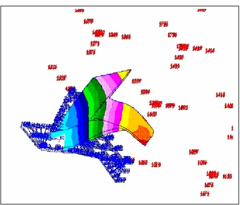
According to this, in the next pages this technique will be introduced to the two models that were defined in the present work; the Solid Hex element model and the Shell-Hex model; simulations on them will be shown in order to verify the validity of the results of Superelements in mechanical and thermal load analysis compared to the original models with no Superelement definition. Validation of this technique will be demonstrated by considering as reference one node which does not belong to the main Superelement; the comparison will be gone on considering Forces and Displacements evaluated on it considering both the full TWF model and the one built using only Superelement. This point of view will be considered both in the mechanical and the thermal simulation as base of comparing. As explained in NASTRAN documentation, it is possible to define superelements as an image or copy of other superelements. This approach was selected for the present study. In this approach a primary superelement is defined. For this primary superelment the detailed finite element model needs to be created and the to be retained nodes in the superelment need to be identified. For the solid element model and the Shell one, different numbers of boundary points were selected because of the different nature of the elements themselves. The following pictures show the different definition of the primary superelement of both models.

Figure 1: Solid primary Superelment

(4)

For all copies (images) of the primary superelement, “only”the boundary nodes have to be defined. In the pictures above they are indicated with the red numbers. To automate this a MATLAB program was written. The functionality of this program will be explained later. Once all the superelements are defined in the bulk data of the MSC/NASTRAN job file (.bdf file), the solution of the model can be performed by NASTRAN which will be able to recognize each superelement introduced.

1. SOLID ELEMENT MODEL.

According to what written above, in this paragraph the application of the Superelement technique will be introduced to the TWF model made up of HEX8 elements which is shown in the picture below.

Figure 3: Solid model

The first step is the definition of a MSC/NASTRAN job file (.bdf file) which is made up of all the data used not only for defining the primary superelement but also to define all the boundary points that will be used to locate all the copies of superelement in the right place. To obtain this a changing was played to the main PCL function in order to define only the data mentioned above; it was necessary to rename all the boundary points because it is necessary to define a way to create automatically all the boundary points maintaining a rational order. The result at this step is shown in the next pictures.

(5)

As it is possible to check in the picture above, only the data used to define the single RUC and the grid points that will be used as boundary points of all the superelements are defined. The new available PCL function is also able to create all the superelement presetting for each specimen that we need because it is defined in a parametric form; the output of this function is shown in the next picture.

Figure 5: Main superelement and boundary points

At this point it is necessary to introduce all the boundary conditions that describe the problem.

Definition of the new job file.

Once the bulk data of the model is created, it is necessary to define the boundary conditions that will characterize the problem. Moreover it still has to be defined both Primary and Secondary Superelements.

Definition of Superelements.

For this step it is necessary to insert in the MSC/NASTRAN job file (.bdf file) the structure that will be now explained. The definition of this organized structure needs to follow a particular order; in fact the same order that was used to define the external points of the primary superelement will have to be used

(6)

when the external points of the secondary superelements will be defined. All the steps necessary to define a right organized job file are shown below.

1 )Primary superelment.

For this step it is necessary to define internal and external points directly in the job file; in particular internal points are defined using the code SESET while the external points are defined using the code CSUPEXT. The next extract from a Nastran job file shows this step:

Figure 6: definition of the primary superelement

2) Defining Copies of Superelements.

The next step is the definition of the copies of the primary Superelement that will be used to define all the complete model. For this it is necessary to define all the external points of the new superelements that will be bounded to the residual structure. It is also important to underline that in this way the Superelement is not right defined because it is necessary to introduce all the external points according to the same order used to define the external points of the primary Superelement. For this, the codes that have to be introduced directly in the Nastran job file are: CSUPER in order to define the new

$############################################################ $ $ CREATING PRIMARY SUPERELEMENT number : 10 $ $############################################################ $

$ definition of the internal points of S.E. 10 $

SESET,10,4,THRU,528 $

$############################################################ $

$ CREATING THE BOUNDARY POINTS OF THE PRIMARY S.E. $ $############################################################ $ CSUPEXT,10,1000,1001,1002,1003,1004,1005,1006 CSUPEXT,10,1007,1008,1009,1010,1011,1012,1013 CSUPEXT,10,1014,1015,1016,1017,1018,1019,1020 CSUPEXT,10,1021,1022,1023,1024,1025,1026,1027 CSUPEXT,10,1028,1029,1030,1031,1032,1033,1034 CSUPEXT,10,1035,1036,1037,1038,1039,1040,1041 CSUPEXT,10,1042,1043,1044,1045,1046,1047,1048 CSUPEXT,10,1049,1050,1051,1052,1053 $

(7)

Superelement and SEQSEP for introducing the right order with which they have to be considered. The next extract from a Nastran job file will clear everything:

Figure 7: Definition of the secondary Superelements.

It is important to underline that this step is very slow if it is made handily; in fact, the number of the GRID POINTS to select and the necessity to maintain the same order could need a lot of time. Because of it, a Matlab routine was written according to the order that all the boundary points follow. It is now enough to give in input to the Matlab function the Length and the Width of a generic specimen to have automatically a file named RUC.dat that it needs to be loaded by Nastran in the job file using the code INCLUDE’RUC.dat’. It is also necessary to have this .dat file in the same folder in which the Nastran job file is created. The following extract is useful to clear every doubt.

$##################################################################### $

$ CREATING IMAGE SUPERELEMENT number : 11 $ $##################################################################### CSUPER,0011,10,1027,1028,1029, 1030,1031,1032,1033,1034, 1035,1063,1064,1065,1066, 1067,1068,1069,1070,1071, 1072,1073,1074,1075,1076, 1077,1078,1079,1080,1081, 1082,1083,1084,1085,1086, 1087,1088,1089,1090,1091, 1092,1093,1094,1095,1096, 1097,1098,1099,1100,1101, 1102,1103,1104,1105,1106, 1107 $ $##################################################################### $

$ CREATING CORRISPONDENCE BOUNDARY POINTS PRIMARY/IMAGE S.E. $ $##################################################################### SEQSEP,11,10,1006,1007,1008,1003,1004, 1005,1000,1001,1002,1009, 1010,1011,1012,1013,1014, 1015,1016,1017,1018,1019, 1020,1021,1022,1023,1024, 1025,1026,1027,1028,1029, 1030,1031,1032,1033,1034, 1035,1036,1037,1038,1039, 1040,1041,1042,1043,1044, 1045,1046,1047,1048,1049, 1050,1051,1052,1053

(8)

Figure 8: loading the RUC.dat file from external source.

3) Ready to start!

After all the steps explained above, it is possible to run the solution. Nastran will automatically create a group of files of which we will take care of the .f06 and the .xdb file. The first one is a file in which it is possible to display any possible FATAL ERROR or WARNING MESSAGE that a non correct definition of the model can give. The xdb file is the solution of the problem that can be loaded directly from Patran. Considering that the bulk data is made up of all that was necessary to define primary superelement and the boundary points, the solution can only be displayed for the primary superelements, while for the rest of the model, actually it is only possible to display the displacement of all the boundary points or the nodal forces involved there. The following picture show an example of deformation of the primary superelement.

$

SOL 101 CEND

SEALL = ALL SUPER = ALL

TITLE = MSC.Nastran job created on 15-Jun-05 at 10:04:22 ECHO = NONE

$ Direct Text Input for Global Case Control Data SUBCASE 1

$ Subcase name : Default SUBTITLE=Default SPC = 2 LOAD = 1 DISPLACEMENT(SORT1,REAL)=ALL SPCFORCES(SORT1,REAL)=ALL STRESS(SORT1,REAL,VONMISES,BILIN)=ALL $ $ $ $######################### $

$ richiama supshell.dat ed imposta $ i parametri di tolleranza $ per l' analisi $ $######################### $ $ BEGIN BULK PARAM POST 0 PARAM CONFAC .5 PARAM AUTOSPC YES PARAM PRTMAXIM YES $

$ $

INCLUDE'RUC.dat' $

(9)

Figure 9: example of deformation of the main superelement.

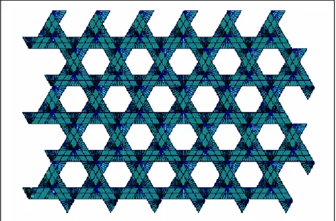
2. SHELL ELEMENT MODEL.

In this paragraph it will be introduced the application of the superelement technique to a TWF model made up of Shell Elements. In this way it will be possible to compare both the Solid and the Shell model in order to evaluate which one has a better behavior; in the next pages all the tests on these two models will be introduced in the detail, results and comments will be explained too. The following picture shows the model that will be considered as reference.

(10)

Figure 10: Shell TWF model

In particular, the same method used for the solid model will be now applied; the first step is again the definition of the single RUC and all what is necessary to define it. Because of the use of Shell elements, this new model will show a significant advantage in what concerns the size of the bulk data required to define the model. The following picture shows the single RUC cell built with only Shell Elements.

Figure 11: Primary superelement.

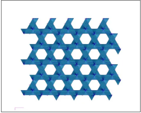
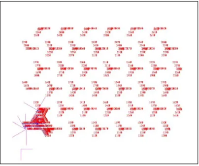
The second step is the definition of a new PCL function which is able to automatically create not only the single RUC but also all the boundary points that will be used in the definition of the Superelements that will build all the specimen itself. In this way it is enough to give in input the size of the specimen to obtain all that is necessary to define a superelement model; the following pictures show all this.

(11)

Figure 12: Superelement model

Figure 13: Primary superelement and boundary points

1)Definition of Superelements.

Now it is possible to define the Primary Superelement that will be used to create all the specimen through copies of it. For this step it is necessary to define internal and external points directly in the job file; in particular internal points are defined using the code SESET while the external points are defined using the code CSUPEXT. The next extract from a Nastran file shows this step:

(12)

Figure 14: definition of the main superelem

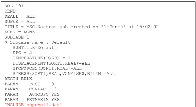
As it was said before, it is important to remember exactly the order with which all the external points are defined by using the code CSUPEXT; that is because in the next step, when copies of the Primary Superelement will be created, a wrong definition of the order of the external points will cause an error during the running. This is the reason for which it was decided to define a Matlab routine which creates a .dat file name supshell.dat made up of all the codes that are necessary to define completely each Superelement; so now it is enough to give in input the Length and the Width of the Specimen and the Matlab function automatically creates the file with the right definition of Superelements to import in the same directory where is the Nastran job file. It is also necessary to load this file directly in the job file through the code INCLUDE as it is shown in the next text box.

Figure 15: including superelement definition from an external source.

$######################################################################## $ $ CREATING PRIMARY SUPERELEMENT number : 10 $ $######################################################################## SESET,10,2,THRU,329 $ $######################################################################## $

$ CREATING THE BOUNDARY POINTS OF THE PRIMARY S.E. $ $######################################################################## CSUPEXT,10,1000,1001,1002,1003,1004,1005,1006 CSUPEXT,10,1007,1008,1009,1010,1011,1012,1013 CSUPEXT,10,1014,1015,1016,1017,1018,1019,1020 CSUPEXT,10,1021,1022,1023,1024,1025,1026,1027 CSUPEXT,10,1028,1029 SOL 101 CEND SEALL = ALL SUPER = ALL

TITLE = MSC.Nastran job created on 21-Jun-05 at 15:02:02 ECHO = NONE

SUBCASE 1

$ Subcase name : Default SUBTITLE=Default SPC = 2 TEMPERATURE(LOAD) = 1 DISPLACEMENT(SORT1,REAL)=ALL SPCFORCES(SORT1,REAL)=ALL STRESS(SORT1,REAL,VONMISES,BILIN)=ALL BEGIN BULK PARAM POST 0 PARAM CONFAC .5 PARAM AUTOSPC YES PARAM PRTMAXIM YES INCLUDE'supshell.dat'

(13)

1) Defining copies of Superelement.

After the definition of the Primary Superelement it is now necessary to define all the other Superelements as copies of the Primary one. For this now it is only necessary to have available all the boundary points that will be used to bound each copied Superelement to the residual structure. In fact a copied Superelements is only made up of all the matrices that describe the Primary Superelement, but it is necessary to define the same number of external points that the Primary Superelement has and also to maintain the same order. For defining a copy of Superelement it is necessary to use the following codes: CSUPER and SEQSEP. With the first code it is defined the new Superelement ID, the source and all the external points of the new Superelement while the second code SEQSEP is necessary to define the correspondent order between the external points of the Primary and Secondary Superelement. Now the Matlab function is also able to create this as it is shown in the following text box taken from the file supshell.dat.

Figure 16: definition of secondary superelements.

$######################################################################## $

$ CREATING IMAGE SUPERELEMENT number : 11 $ $######################################################################## CSUPER,0011,10,1015,1016,1017, 1018,1019,1035,1036,1037, 1038,1039,1040,1041,1042, 1043,1044,1045,1046,1047, 1048,1049,1050,1051,1052, 1053,1054,1055,1056,1057, 1058,1059, $ $######################################################################## $

$ CREATING CORRISPONDENCE BOUNDARY POINTS PRIMARY/IMAGE S.E. $ $######################################################################## SEQSEP,11,10,1004,1003,1002,1001,1000, 1005,1006,1007,1008,1009, 1010,1011,1012,1013,1014, 1015,1016,1017,1018,1019, 1020,1021,1022,1023,1024, 1025,1026,1027,1028,1029 $

(14)

2) Ready to start!

After all the steps explained above, it is possible to run the solution. Nastran will automatically create the same group of files that was introduced before. Considering that the bulk data is made of all that was necessary to define primary superelement and the boundary points, the solution can only be displayed for the primary superelements, while for the rest of the model, actually it is only possible to display the displacement of all the boundary points or the nodal forces involved there.

(15)

TESTING AND COMPARING SUPERELEMENT MODELS

In this second part of the section, both the Solid and the Shell TWF models will be subjected to mechanical simulations and the results will be compared to the ones obtained with the Superelement models. In particular the target of this final part is to compare the results from a model with no definition of Superelements in it with those obtained from the same model but made of only Superelements; in this way it will be possible to verify if the Superelement technique is consistent and can be used confidently in future works.

3. MECHANICAL SIMULATION TESTS.

In this paragraph a mechanical test simulation will be introduced, that will be considered as reference for a comparison between models with and without Superelements. It is important to underline that because of the definition of a model with Superelement technique, it is only possible to define external loads on its external points; actually this is a limit in the use of this new technique. Anyway it was considered as reference a simple case of uniaxial load for which one side of the specimen is completely fixed and the opposite side is subjected to a displacement of given value. It was chosen to consider a displacement in the X direction and so to have at the end a rather faithful simulation of the E1 modulus test that it was performed in the previous sections. The way to go on will be to start with the original model with no Superelement in it, to continue with the corresponding Superelement model and to compare the results.

4. SOLID HEX8 MODEL.

(16)

Figure 17: Solid model

The material properties are the same used until now, a Carbon Epoxy impregnated yarn with characteristic of transversely isotropic material. The boundary conditions applied are: u = v = w = 0 on the left side of the specimen and u = 0.001 mm and v = w = 0 on the opposite side. The following pictures show the boundary conditions; they will be repeated for each model.

U = V = W = 0 U = 0.001 m V = W = 0

Figure 18:boundary conditions.

The results are evaluated in terms of reactions (N) on the fixed side of the specimen and displacement (mm) on a node chosen as reference.

(17)

(REACTION on the fixed size of the 5x6 URC specimen) • Fx = - 0.49422 • Fy = - 0.0345 • Fz = 7.89E-05

(DISPLACEMENT evaluated on the node 12830)

• X = 0.0003817 • Y = 0.0002855 • Z = 0.00056385

5. SUPERELEMENT SOLID MODEL.

The same test will be applied to a 5x6 RUC Solid model made up of only Superelments.

Figure 19: primary superelement

(18)

In the pictures above is it possible to see the Primary Superelement and the whole specimen made of the primary superelment and all the external points of the other superelements defined as copies of the primary. The boundary conditions that will be applied are the same of the Full Solid Model; in particular the correspondent node will be taken as reference in order to compare the results between these two models. The node considered is the node 2603. The red arrow (see pictures above) links to the node location which will be considered as reference for all the following simulations. The results can be displayed in terms of deformation of the Primary Superelement and not of all the specimen; this is because the data base is only made of all the elements used to build the single RUC cell and the boundary points, but it is possible to know the displacement or the force on a node that is defined as external point. Actually the limit of this technique is that it is not possible to display all the deformation of the specimen or to know the displacement of a node which is internal to a Superelement defined as copy of the Primary; this is an interesting point for a future work. The following picture show the deformation of the Primary Superelement; it is only an example of what in reality it is possible to display using Superelements, so for the Shell Superelement model it will be omitted.

Figure 20:deformation of the primary suprelement

The results obtained for this model are shown below in term of reaction on the fixed side of the specimen (evaluated as summation of all the nodes fixed) and displacement of the node considered as reference.

(19)

• X = 0.0003818 • Y = 0.0002853 • Z = 0.00056057

It is important to underline that the node that was taken as reference does not belong to the Primary Superelment; this is because it is interesting to verify what is the behaviour in terms of Secondary Superelements; in other words the target of this test is to verify the difference in terms of force and displacements between a full model and the correspondent model defined with Superelements. Looking at the results and comparing them, it is possible to observe that the Superelement technique gives excellent results when it is applied to the TWF specimen in problems in which forces or displacements are the target; in fact the difference between the two results is really low.

6. SHELL CQUAD4 MODEL.

The same steps will be now followed for a specimen of the same size of the solid model but made up of Shell CQUAD4 elements. The specimen that will be introduced consists of shell elements for the

(20)

yarns with HEX8 elements added in the cross section defined with the resin properties; this is an unreal configuration. The following picture shows the specimen and the cross section itself.

In the same way of the other models, the same boundary condition will be applied in order to compare the results with the results obtained with the Solid and Superelement Solid models. The following pictures show the configuration.

U = V = W = 0 Figure 21: boundary conditions U = 0.001mm V = W = 0 Zoom of the Cross section

Made up of HEX8 solid Element with resin properties

(21)

Again the results are evaluated in terms of reaction on the fixed side of the TWF specimen and the displacement of the corresponding node (as for the other model, the node considered as reference is in the same location for each model). In particular for this example the node 13606 will be considered as reference.

• X = 0.000329 • Y = 0.0003548 • Z = 0.00031481

It is important to underline that the behavior of this model doesn’t represent the real one because the cross section is made not only of Shell elements, but also of Hex elements defined with the resin properties; it means that we are adding something that doesn’t exist in the reality. The results displayed above refer to the case in which the resin has its own real properties defined in each Hex element; as it is possible to verify, the values of the displacements are quite different if compared to the values obtained with the Solid model.

7. SUPERELEMENT SHELL MODEL

The Superelement technique will be now applied to the Shell model. The same steps used to create the Superelement model of the Solid Element model will be applied, so only the pictures will be shown

(22)

because the way to define this new model is exactly the same. The Superelement model will appear as follows.

Figure 22: Superelement shell model and primary superelement

The boundary conditions are exactly the same applied to the other models and the results are evaluated in terms of reaction on the fixed side and displacement on one node. In particular the node 1890 is chosen as reference in order to be compared to the displacement evaluated in the other models.

Primary Superelement Made up of CQUAD4 And HEX8 elements

(23)

(REACTION on the fixed size of the 5x6 URC specimen) • Fx = - 0.52646

• Fy = - 0.047119 • Fz = 2.7188E-05

• X = 0.000329 • Y = 0.0002708 • Z = 0.000427

In the table below it is possible to look at the summary of the results.

Fx (N.) Fy Fz X (mm) Y Z

Full Solid - 0.49422 - 0.0345 7.89E-05 0.0003817 0.0002855 0.0005638 Sup.Solid - 0.49444 - 0.03449 7.957E-05 0.0003818 0.0002853 0.0005605 Full Shell - 0.5295 - 0.04755 4.017E-05 0.000329 0.0003548 0.00031481 Sup.Shell - 0.52646 - 0.04711 2.718E-05 0.000329 0.0002708 0.000427

Table 1: summary of the results.

It is important to make comments about the Superelement technique, applied on both the Solid and the Shell model. Looking at the results, it is possible to observe that the Solid model seems to behave better than the Shell model; in fact the difference in the results evaluated going from a full Solid model to a Superelement Solid model is really low, while with the Shell model we have a higher difference in the results, specially in the out-of-plane behavior, both the Fz reaction and the Z displacement of the node chosen as reference; the cause of this error may be the particular out-of-plane behavior of the shell element or a too complicated geometry of the model. The next part of this section is about the application of a nodal temperature on all the specimens instead of a displacement or a force. This contest will involve a different way to define the load in the Superelement technique as it will be shown

(24)

8. NODAL TEMPERATURE TEST

In this new paragraph, an analysis will be introduced in which a Temperature will be defined on nodes instead of a nodal force or displacement. The aim of this analysis is to verify if the Superelement technique is still consistent also for a load case like this. This is because a Temperature defined on a node is totally different from a nodal force or a displacement in the way it is considered. Again the analysis will be performed starting from the full model and going to the Superelement model for both solid and shell model and in each case a nodal temperature of 100 C will be applied to all the specimen. The boundary condition that will be applied consists of zero degrees of freedom on one side of the specimen while the remaining part of the model is free to deform; results will be evaluated in terms of displacement in one node whose location will be considered as reference in each model through all the analysis.

9. SOLID ELEMENT MODEL

A temperature defined on node will be applied to all the specimen; the specimen is made up of 5x6 RUC cells and the temperature applied is of 100 C. The starting model is the same one used in the previous paragraph, made up of HEX8 elements with Carbon Epoxy impregnated material property defined as transversely isotropic .In the following picture it is possible to look at the specimen and the temperature defined on it.

(25)

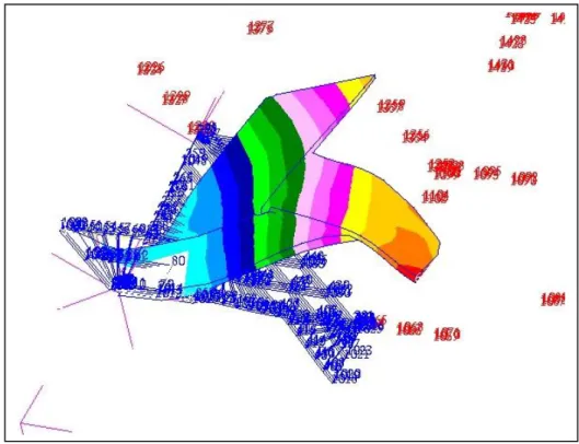
The results are evaluated in terms of displacement of the node chosen as reference. The following picture shows the deformation of the specimen under temperature.

Figure 24: Deformation under the temperature

As it is possible to see there is out of plane deformation, but this deformation has a less twist involved than the deformation of the RUC caused by a displacement applied on nodes. The results in term of displacements are shown below.

(DISPLACEMENT evaluated on node 12830) • X = 0.0014248 • Y = - 0.000146 • Z = 0.07178

(26)

10. SUPERELEMENT SOLID MODEL

The same method will be now adapted to a Superelement Solid model. The definition of a model like this creates some problems in the application of the nodal temperature. In particular, it is not sufficient to define the temperature in one node, but it is also necessary to indicate the element to which the node belongs; because of this, to define a temperature to all the nodes of the model is difficult when copies of Superelement are used. This is because a copy of a Superelement, by definition, does not have any Solid element or grid point in it. Because of this, it is necessary to define a nodal Temperature only for all the points that characterize the Primary Superelement in term of both external and internal points. In this way, being all the other Superelements defined as copies of the Primary one, all the conditions applied directly to the Primary Superelement will be automatically applied to all its copies. The results in terms of displacement (mm) are shown below.

(DISPLACEMENT evaluated on node 2603)

• X = 0.0013808 • Y = - 0.000158 • Z = 0.0574

(27)

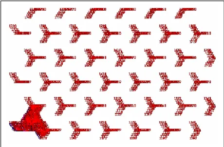
11. SHELL ELEMENT MODEL

Following the same steps introduced for the past models, it will be considered a Shell element model made up of CQUAD4 elements; the same temperature of 100 C and boundary condition will be applied. The following picture shows both the temperature and the boundary condition on the model.

U = V =W = 0 T = 100 C (each node)

Figure 25: temperature on nodes and boundary conditions

The results are shown below; the node 13606 is chosen as reference in order to compare the results with the previous analysis. It is important to underline the rule of the resin which is locate in the cross section through HEX8 elements considering the value of the CTE.

(28)

• X = 0.000405421 • Y = 0.00032457 • Z = 0.029575754

Again, if the contribution of the resin is reduced to zero assigning a CTE = 0 to the resin properties the following results are found.

• X = 0.001451 (CTE = 0) • Y = - 0.0000522 (CTE = 0) • Z = 0.0429 (CTE = 0)

In this way the values obtained are closer to the values obtained with the solid model; this is because the Shell model has in the cross section more resin than the real quantity because of the HEX8 elements inside defined with resin properties. It is important to underline the difference that we have especially in the out-of-plane component; 0.0429 instead of 0.07 for the solid model. This is a quite large difference whose reason will be explained later with other analysis. The conclusion will be that the Shell model does not behave correctly when a nodal temperature or in general a thermal load is applied on the model. This occurs for two reasons: 1) Shell elements are not able to feel dilatation through the thickness when a temperature is applied on them. 2) When the geometry of the model is too complicated like the TWF geometry itself, errors in the tolerance are inevitably involved.

(29)

12. SUPERELEMENT SHELL MODEL

Following the same method adopted in the previous test, a Superelement shell model will be now subjected to the same temperature load and boundary conditions. The results in term of displacement on one node chosen as reference are shown below.

• X = 0.0004577902 • Y = 0.0003069347 • Z = 0.04431

These are all values obtained considering the total contribution of the resin with its properties. The results evaluated assigning a CTE = 0 to the resin in order to simulate the real behavior in the cross section are shown below.

• X = 0.001457 (CTE = 0) • Y = 0.041077 (CTE = 0) • Z = - 0.0000529 (CTE = 0)

Looking at the values above, it is important to underline that the Superelement technique seems to better behave with the Solid model than the Shell one; in fact despite the errors are lower in the Shell

(30)

thermal load for the reasons that will be introduced in the following pages. To conclude this first part of analysis a table with all the results evaluated with a nodal temperature static analysis is shown below.

Table 2: summary of the results.

13. ANALYSIS WITH NODAL TEMPERATURE

In the following paragraph it will be explained the cause of the different values obtained with a full model and a Superelement model when a nodal temperature is used. In particular tests on simple geometries will be introduced, in order to understand what is the reason of such behavior, both in the Solid and the Shell model, and comments and conclusion will be added at the end of this new analysis. The first important aspect to underline is the need for an appropriate choice of the element to use when a temperature is introduced in the model. So the first question that will be answered is the following.

• Shell or Solid Element?

To answer this question the following analysis will be performed with the aim to discover which is the element that better behaves under a thermal load.

T = 100 C X (mm) Y Z

Full Solid 0.0014248 - 0.000146 0.07178 Sup.Solid 0.0013808 - 0.000158 0.0574 Full Shell 0.000405421 0.00032457 0.029575754 Sup.Shell 0.000457790 0.000306934 0.04431 Full Shell cte = 0 0.001451 - 0.0000522 0.0429

(31)

13.1 Solid model

A simple example is built with only HEX8 elements; the properties are the same used until now, so we are considering an Impregnated Carbon Epoxy set of properties. The example is made up of few solid elements in order to have a very quick and easy model to run. A temperature of T = 100 C is applied homogeneously and the left side of the model is fixed. Again a node whose location will be considered as reference is chosen. The following picture shows the configuration chosen as reference.

Figure 26: easy geometry.

The following picture shows both the temperature and the boundary conditions introduced.

Figure 27: temperature on nodes and boundary conditions.

(32)

The following picture shows the deformation of the model under the applied temperature.

Figure 28: deformation under temperature.

The results in term of the displacement of a node chosen as reference are shown below.

• X = -7.55676E-5 • Y = 0.00119

(33)

13.2 Superelement Solid model.

Now it will be followed the same method but working on the corresponding superelement model. The following pictures show both the definition of the superelement and the deformation under the applied temperature; obviously both temperature and the boundary condition are the same used in the full solid model.

Figure 29: definition of the main superelement and the secondary superelement

Figure 30: deformation under the temperature.

As it is possible to see in the pictures, only the primary superelement can display its deformation because of the way with which a Copied Superelement is defined. The results in term of displacement of the same node 20 chosen as reference are shown below.

(34)

• X = -7.55676E-5 • Y = 0.00119

• Z = -0.00041

The results reveal that the values of the displacements evaluated on the node with the same location in a full model and in a model made up of superelements are exactly the same. The reason of the error that it was revealed testing the TWF specimen has to be related to the complex geometry of the specimen itself. In fact a complicated geometry involves the necessity to change the tollerance in the NASTRAN job file, because of small errors of orientation of the boundary points of the secondary superelements.

13.3 Shell element.

All the steps introduced above are going to be repeated in the same way for the same example created using only shell element; CQUAD4 element. The material is exactly the same used in the solid model as well as the boundary conditions and the nodal temperature load. The following pictures show the procedure step by step.

Figure 31: Shell element model

(35)

Figure 32: boundary conditions

U = V = W = 0

Figure 33: deformation under temperature.

The results are shown below in term of displacement of the node 20.

• X = -8.48147E-5 • Y = 0.001192

(36)

It is important to underline that the Shell model gives results that are not able to feel the out of plane deformation caused by the temperature; this is because of the definition of Shell element itself. So it is possible to say that the Shell model does not represent faithfully the behavior of the real model and for this reason it cannot be used to model the TWF specimen when a temperature is applied.

13.4 Superelement Shell model

Following the same procedure introduced with the solid model, a Superelement model can be defined, made of shell element. Obviously both the boundary conditions and the nodal temperature load are exactly the same applied in the previous analysis. The following pictures will show the procedure step by step.

Figure 34: superelement definition

(37)

Again the results are evaluated in terms of displacement of the node 20.

• X = -8.48147E-5 • Y = 0.001192 • Z = 0

Also in this case the application of the superelement technique to the Shell model does not give any error; in fact the values of the node 20 are exactly the same with both models. The conclusion is that the error that is revealed testing the TWF specimen is caused by the complex geometry that characterizes the single RUC itself and so all the specimen to. The following table summarizes all the values obtained from this analysis in order to allow comments about it.

Table 3: summary of the results with simple geometries.

Looking at the results it is possible to say that the Superelement technique gives good results, but its limit is the geometry that is involved in the model. In particular, with simple geometries it is possible to use the superelement definition without errors, so the consistence of this technique is really good. On the other side, when complex geometries must be modeled, an unavoidable error is revealed comparing the results; analysis were done trying to discover the reason and, as it was said before, the only reason is the geometry itself. Speaking about the quality of the solutions, it is possible to say that they are really good if nodal displacement or forces are used; in fact the previous analysis revealed that the results of the full model and the superelement model were really close.

Otherwise, if a nodal temperature is defined, while the x-y displacement components are good, the z one reveals an error of more or less 15%. The reason is again linked to the complex geometry used. It

T = 100 C X (mm) Y Z

Full Solid -7.55676E-5 0.00119 -0.00041 Sup.Solid -7.55676E-5 0.00119 -0.00041 Full Shell -8.48147E-5 0.001192 0 Sup.Shell -8.48147E-5 0.001192 0

(38)

other words, shell elements are not able to simulate correctly the TWF behavior because they are not able to feel the dilatation involved through their thickness. The conclusion About Superelement technique is that this technique can be applied with good results if the geometry of the model is not so complex like the TWF specimen. It does not mean that this technique is not correct, but that the results can reveal a small error if the model has a too complex geometry. Anyway the advantage in terms of model time reduction is really relevant so the conclusion is that this technique can be used to model large surfaces for a first time analysis.

14 A MORE DETAILED ANALYSIS

In the previous analysis the main conclusion was that the solid element better behaves in problems that involve temperature because it has the ability to consider the deformation through the thickness of the model. In this paragraph, a more detailed analysis will be performed; in particular it will be considered only a solid model but more detailed; the geometry will have the aim to simulate something similar to the cross region of the TWF model. New boundary conditions will be applied in order to cause twist in the cross section of the new specimen; the target of this new analysis is to verify if the error in the out-of-plane direction that we have using superelements in the TWF specimen is related to the behavior of the cross section when a temperature is applied on all the specimen. The same temperature of T = 100 C will be used as well as the material properties (Impregnated Carbon Epoxy). The following pictures will show in the detail the configuration.

Figure 36: new geometry set.

For this new example three sides of the specimen are completely fixed as it is possible to see in the next picture.

(39)

Figure 37: new boundary conditions.

U = V = W = 0

The next picture shows the deformation of the model under the applied temperature; it is interesting to underline the twist effect in the cross region and the out of plane deformation of the model itself.

Figure 38: deformation of the model.

Figure 39: lateral view of the deformed configuration.

(40)

• X = 0.0001056 • Y = -0.0011208 • Z = -0.0013370

• X = 0.0001555 • Y = 0.0009979 • Z = -0.0016301

• X = 0.0003918 • Y = 0.0001603 • Z = 0.0010393

(41)

14.1 Superelement Solid Model.

The same method applied for the solid model introduced before will be now applied to the correspondent superelement model. In particular a Primary superelement will be defined and the other one will be created as copy of it. The same temperature and the same boundary conditions will be used. The following pictures show the configuration.

Figure 40: superelement definition.

(42)

Again the results are shown below in terms of displacement on the same nodes.

(DISPLACEMENT evaluated on node 274) • X = 0.0001056

• Y = -0.0011208 • Z = -0.0013370

• Y = 0.0009979 • Z = -0.0016301

• Y = 0.0001603 • Z = 0.0010393

As it is possible to see, the results are exactly the same obtained with the full model. So the errors revealed in the TWF specimen have to be related to other reasons which have still to be explained. One reason can be the too complex geometry which characterizes the TWF unit cell; in fact applying Superelement technique to a TWF specimen, MSC/NASTRAN underlined an error linked to a difference in the orientation between primary and secondary superelement boundary points. Anyway this does not mean that the geometry is the real and unic cause of the problem; other reasons could be found about this; for example it could be considered if the number of the boundary points is enough to completely define the location of the secondary Superelement.

Anyway thanks to the analysis that was introduced in this section, important results were found. Comments can be added about the use of Solid, Shell and Superelement technique in linear static analysis. In fact looking at the tables shown in this section it is possible to check which element better behaves under displacement, forces and temperature; the Shell element which involves a lower number of degree of freedom reveals quite good values for displacement and force loads, while it shows a non perfect behaviour under temperature for the reason explained before. On the other side, the use of Solid element involves a higher number of degrees of freedom but at the same time it gives more

(43)

faithful values if it is considered that also under a temperature load it is able to show deformation through the thickness. So the first conclusion is that, according to the problems revealed by a thermal load, the Solid element is recommended in the modelling of a geometry like the TWF. The tables also permit to make comments about Superelement models; the values obtained and the tests introduced in this section in order to understand the reason of the differences in displacement components allow us to say that Superelement technique gives very good results but depending on the load case used. In fact, while this technique gives very good results for mechanical loads, on the other side it has to be used with precautions when thermal loads are defined.

The gain in terms of bulk data weight is really relevant if compared to the one of the model with no superelement definition.

About computing time, it was not found any gain; the reason of this has to be linked to how NASTRAN defines the secondary superelements. In fact it should be analyzed if the secondary superelement is defined in terms of reduced matrices or not. In the first case, a large advantage in computing time should be found, while in the second case computing time should be the same of the full detailed model.

It is important to add that actually the limit of this technique is that it is not possible to display directly the deformation of all the specimen or any other results which are related to points that belong to a superelement defined as a copy of the Primary one; this is a good point on which to work for the future. The idea is that it could be possible to obtain all the matrices that describe the entire model so, starting from them, it should be possible to obtain the behaviour of each node of the model.

Concluding it is important to underline for a future work that a more detailed Hex element RUC cell is recommended; in fact thanks to the superelement technique it is possible to define a very detailed single RUC, to define it as Primary Superelement and then to build the specimen defining copies of it; in this way the solution is expected to be very detailed and close to the correct one. Another interesting application of Superelement technique could be the definition and the use of external superelement in the simulation of large surfaces like an antenna reflector.