PAPER • OPEN ACCESS
Optimal Gaussian metrology for generic multimode interferometric circuit
To cite this article: Teruo Matsubara et al 2019 New J. Phys. 21 033014
View the article online for updates and enhancements.
PAPER
Optimal Gaussian metrology for generic multimode interferometric
circuit
Teruo Matsubara1
, Paolo Facchi2,3
, Vittorio Giovannetti4
and Kazuya Yuasa1,5
1 Department of Physics, Waseda University, Tokyo 169-8555, Japan 2 Dipartimento di Fisica and MECENAS, Università di Bari, I-70126 Bari, Italy 3 INFN, Sezione di Bari, I-70126 Bari, Italy
4 NEST, Scuola Normale Superiore and Istituto Nanoscienze-CNR, I-56127 Pisa, Italy 5 Author to whom any correspondence should be addressed.
E-mail:[email protected]
Keywords: quantum metrology, quantum estimation, quantum Fisher information, Gaussian states, squeezed states, optical circuits
Abstract
Bounds on the ultimate precision attainable in the estimation of a parameter in Gaussian quantum
metrology are obtained when the average number of bosonic probes is
fixed. We identify the optimal input
probe state among generic
(mixed in general) Gaussian states with a fixed average number of probe
photons for the estimation of a parameter contained in a generic multimode interferometric optical circuit,
namely, a passive linear circuit preserving the total number of photons. The optimal Gaussian input state is
essentially a single-mode squeezed vacuum, and the ultimate precision is achieved by a homodyne
measurement on the single mode. We also reveal the best strategy for the estimation when we are given L
identical target circuits and are allowed to apply passive linear controls in between with an arbitrary
number of ancilla modes introduced.
1. Introduction
Quantum-mechanical features and quantum effects can drastically improve the accuracy of measurements [1–6]. This is known as quantum metrology, and is one of the promising future quantum technologies. In
particular, quantum optical measurement schemes using photonic probes have recently been under intense study[1,3–6], pursuing strategies that allow to beat the standard quantum limit on the measurement accuracy,
both theoretically[7–64] and experimentally [65–81].
In a variety of quantum optical metrology settings, the probe sensitivity to the target parameter can be improved by squeezing the state of the input light[7,8]. Entanglement is also an important keyword in the studies of quantum
metrology[4–6]. In these ways, the state of the input probe photons is important for high precision metrology.
There is an interesting class of states of light: Gaussian states. From a practical point of view, a variety of Gaussian states are relatively easy to generate in laboratories, and various quantum information tasks have been implemented experimentally using photons in Gaussian states[82–84]. Also from a theoretical point of view,
they provide an interesting category of quantum information protocols[82–84]. For these reasons, quantum
optical metrology with Gaussian input probe states and/or Gaussian channels has been eagerly investigated [14,16,17,19,21,25,28,29,32,34,36,43,45–47,49,51,55,59–61,64].
For instance, the estimation of a single-mode phase shift is studied with pure[14] and mixed [19] Gaussian
probes, and some other single-mode Gaussian channels such as squeezing and amplitude-damping are analyzed with general mixed Gaussian probes[34]. The estimation of a single-mode phase shift with general mixed Gaussian probes
is discussed in the presence of general Gaussian dissipation[60]. A few specific mode Gaussian channels like
two-mode squeezing and two-mode mixing are studied with some particular types of two-two-mode Gaussian probes[59]. The
ultimate precision bound is clarified for generic two-mode passive linear circuits, which preserve the number of photons passing through them(they are Gaussian channels) [47]. A formula for the quantum Fisher information
(QFI) valid for any multimode pure Gaussian states is derived and investigated under the condition of intense probe OPEN ACCESS
RECEIVED
15 November 2018
REVISED
25 January 2019
ACCEPTED FOR PUBLICATION
11 February 2019
PUBLISHED
19 March 2019
Original content from this work may be used under the terms of theCreative Commons Attribution 3.0 licence.
Any further distribution of this work must maintain attribution to the author(s) and the title of the work, journal citation and DOI.
light(with large displacement) [25]. General multimode Gaussian unitary channels (Bogoliubov transformations) are
considered with pure probe states not restricted to Gaussian states and the behavior of the QFI for large mean photon numbers is discussed[46]. A formula for the QFI matrix is derived for general multimode Gaussian states and
multiparameter Gaussian quantum metrology is discussed[61,64].
In this paper, we study the estimation of a parameter embedded in a generic M-mode passive linear interferometric circuit, and clarify the ultimate precision bound achievable with Gaussian probes. We identify the optimal input probe state among all Gaussian states(including mixed Gaussian states) with a fixed average number of probe photons. Such a bound is known for M=2 [47], but is not known for M 3. The proof
strategy taken for M=2 is not helpful for M 3, and it is not a simple generalization of the previous work. More specifically, we will consider the setting shown in figure1: a collection of M photonic modes is employed as a probe to recover the value of an unknown parameterj, which is imprinted on the state of the probe via the action of a passive(i.e. photon number preserving), Gaussian (i.e. mapping Gaussian input into Gaussian output), unitary transformation Uˆ . Under the assumption that the allowed input density matricesj rˆ of the M modes belong to the set(M N, )of(not necessarily pure) Gaussian states with an average photon numberN, we are interested in the ultimate accuracy in the estimation ofj attainable when having full access to the output state
U U . 1.1
rˆj= ˆ ˆ ˆjr j ( )
†
Our main result consists in showing that, irrespective of the explicit form of Uˆ , the minimum value of thej uncertainty dj on the estimation ofj is bounded from below by the Heisenberg-like scaling
N
1 . 1.2
min
dj ( )
To this end, we shall focus on the QFI F j r( ∣ ˆ )of the problem, which, via the quantum Cramér–Rao inequality [1,4,85–90], sets a universal bound ondjminthat is independent of the adopted measurement procedure,
F 1 . 1.3 min dj j r ( ∣ ˆ ) ( )
We hence prove(1.2) by showing that the maximum value of F j r( ∣ ˆ )attainable on the set(M N, )is bounded by a quantity which scales quadratically inN, namely,
F j r 8 g 2N N +1 , " Îr M N, . 1.4
j
( ∣ ˆ ) ( ) ˆ ( ) ( )
Here, g is the spectral norm of the Hermitian matrixj
g iU dU
dj , 1.5
=
j j† j ( )
with Ujbeing the unitary matrix describing the circuit, defined in(2.2), and is independent of the input staterˆ. Moreover, we show that the bound(1.4) is sharp and can be saturated. In fact, we identify the optimal states
within(M N, )that saturate the inequality(1.4): they are pure statesropt=∣yoptñáyopt∣given in(3.31). We note that, apart from some special cases, such optimal vectors∣y ñopt generally depend on the variablej, whose unknown value we wish to determine. Therefore, the possibility of using this optimal input state for achieving the bound is not straightforward, and would require in practice the use of iterative procedures with a sequence of input states that approximate the optimal state. Anyway, the optimal state∣y ñopt enables us to reach the upper bound(1.4).
The paper is organized as follows. The model and the estimation problem are set up in section2. In section3, the maximal precision achievable by a Gaussian probe is found,first for pure Gaussian states and then for mixed Gaussian states. Moreover, we explicitlyfind the optimal states that achieve the maximal precision. Two different measurement schemes are presented in section4. We look at a few simple examples in section5.
Figure 1. The generic passive linear optical circuit Uˆ with M input ports and M output ports. Our problem is to estimate a parameterj
j contained in the circuit Uˆ , by sending probe photons through it and measuring its output. We will restrict ourselves to Gaussianj
input states rˆ with a given average number of probe photons Ná ñ =ˆ N, among which we identify the best Gaussian states reducing the accuracy limit in the estimation ofj as much as possible.
Furthermore, in section6, we exhibit the optimal sequential strategy for the estimation when several target circuits, together with ancilla modes, are allowed to be used. A summary of the present work is given in section7. We add four appendices, containing some technical tools and proofs. In appendixAwe collect some results on Gaussian states and operations, in appendixBwe show the derivation of a formula for the QFI, in appendixCwe prove some inequalities on Hermitian matrices used in the solution of the optimization problems, and
appendixDcontains the proof of the optimality of the measurement scheme presented in section4.
2. The model
Let us consider a set of M bosonic modes described by the operators aˆmandaˆm†satisfying the canonical commutation relations
am,an =0, am,an =dmn m n, =1,¼,M . 2.1
[ ˆ ˆ ] [ ˆ ˆ ]† ( ) ( )
The passive Gaussian unitary Uˆ ofj figure1is defined by the mapping [82,84]
U a Um U a m 1, ,M , 2.2 n M mn n 1
å
= = ¼ j j j = ˆ ˆ ˆ† ( ) ˆ ( ) ( )or simply written asUˆ ˆ ˆj†aUj=Ujaˆwith aˆ =( ˆa1 aˆM )T, where Ujis an M×M unitary matrix, whose functional dependence uponj is assumed to be smooth. We remind that this kind of transformation preserves the total number of photons of the system, i.e.
U NU N, N a a , 2.3 m M m m 1
å
= = j j = ˆ† ˆ ˆ ˆ ˆ ˆ ˆ† ( )and can be constructed by using beam splitters and phase shifters.
Our problem is to estimate the actual value of the parameterj embedded in Uˆ by probing the output statej
rˆjin(1.1). Consider hence a generic positive operator-valued measure (POVM) = P{ ˆ }s s[91,92] producing measurement outcomes s with probabilities
p s( ∣ )j =Tr( ˆ ˆ )Psrj. (2.4)
The Cramér–Rao inequality [1,4,85–90] establishes that any attempt at estimating j from the values of s is
characterized by an uncertainty F 1 , , 2.5 dj j r ( ∣ ˆ ) ( ) with F , p s lnp s 2.6 s 2
å
j r j j j = ¶ ¶ ⎛ ⎝ ⎜ ⎞ ⎠ ⎟ ( ∣ ˆ ) ( ∣ ) ( ∣ ) ( )being the Fisher information(FI) of the process. A stronger, universal bound on the attainable estimation error can now be obtained by optimizing the right-hand side of(2.5) with respect to all possible POVMs. This yields the quantum Cramér–Rao inequality(1.3), with
F maxF , 2.7
j r = j r
( ∣ ˆ ) ( ∣ ˆ ) ( )
being the QFI of the problem, which by construction depends only upon the input staterˆand the circuit Uˆj [1,4,85–90]. The maximization in(2.7) can be analytically solved, yielding the following compact expression
F( ∣ ˆ )j r =Tr( ˆ ˆ )rj jL2 , (2.8)
with Ljˆ being a Hermitian operator called symmetric logarithmic derivative(SLD), satisfying
L L d d 1 2 . 2.9 r j = r +r j j j j j ˆ ( ˆ ˆ ˆ ˆ ) ( )
The goal of the present work is to optimize the value of the QFI F j r( ∣ ˆ )in(2.8) with respect to a special class
of allowed input statesrˆ. In particular, we shall restrict the analysis to the set(M N, )of M-mode Gaussian states with afixed average photon numberN, i.e.
N N
Tr( ˆ ˆ )r = . (2.10)
This last condition is motivated by the fact that it is not realistic to consider probing signals with unbounded input energy. It turns out that for generic(non-Gaussian) input states the constraint(2.10) is not strong enough
optimal values for F j r( ∣ ˆ )requires to impose an extra condition on the variance ofNˆonrˆ;see also[27]), yet for
Gaussian inputs this suffices and the QFI F j r( ∣ ˆ )isfinite under the constraint(2.10).
3. Optimization of QFI
As recapitulated in appendixA, an input staterˆbelonging to the Gaussian set(M N, )is fully characterized by a( M2 ´2Mreal, symmetric, and positive-definite) covariance matrix Γ with matrix elements
z z z z m n M
1
2 , , 1, , 2 3.1
mn m n m n
G = á{ˆ ˆ }ñ - á ñá ñˆ ˆ ( = ¼ ) ( )
and a( M2 real column) displacement vector
d= á ñzˆ (3.2)
which satisfy the constraint(2.10), i.e.
d N 1 2Tr 1 2 1 2 , 3.3 2 G - + = ⎜ ⎟ ⎛ ⎝ ⎞⎠ ( )
where zˆ=( ˆ ˆ)x yTis the quadrature operator vector with x a a 2
m= m+ m
ˆ ( ˆ ˆ )† and yˆm=( ˆam-aˆ )m† 2 i (m=1,¼,M), and á ñ denotes the expectation value onrˆ. Furthermore, since Uˆ is a passive Gaussianj unitary, the associated output staterˆjobtained as(1.1) also belongs to M N( , ), and its covariance matrix Gj and displacement vector djdepend linearly onΓ and d, as
d d
R RT, R , 3.4
G =j jG j j= j ( )
where Rjis the orthogonal matrix rotating the quadrature operators according to Uˆj(see appendixA). Under this condition, the SLD fulfilling(2.9) can be expressed as [29]
z d z d d z d L T Tr , 3.5 T 1 j = - L - + ¶ ¶ G - - L G j j j j j j- j j j ˆ ( ˆ ) ( ˆ ) ( ˆ ) ( ) ( )
and, accordingly, the QFI reads[29,93]
d d F Tr . 3.6 T 1 j r j j j = L ¶G ¶ + ¶ ¶ G ¶ ¶ j j j j- j ⎛ ⎝ ⎜ ⎞⎠⎟ ( ∣ ˆ ) ( )
Here,Ljis the solution to
J J J J J i 2 i 1i 2 i 1 2 i 1, 3.7 j L - G L G = -¶ G ¶ j j - j j - j -( ) ( ) ( ) ( )
with J being the M2 ´2Mmatrix
J 0 0 , 3.8 =
-(
)
( )known as the symplectic form.
In the remainder of this section, we shall employ these expressions to derive the inequality(1.4). The analysis
will be split into two parts, addressingfirst the case of the pure elements of M N( , )and then the case of the mixed ones. For those who are familiar with QFI optimization problems, this procedure might sound unnecessary. Indeed, due to the convexity of QFI[4,94], it is well-known that pure input states perform better
than mixed input states for metrological purposes. We cannot, however, apply the same argument in the present case, and it is not obvious atfirst glance whether the best state is a pure state. Indeed, even though it is true that any mixed Gaussian state can be decomposed as a convex sum of pure Gaussian states, each of the constituent of such decomposition does not necessarily satisfy the constraint(2.10) on the photon number in general. In short,
the Gaussian set(M N, )is not a convex set, and therefore we cannot use the convexity argument to optimize the QFI. As a consequence, for the problem we are considering here, we have to address explicitly the case of mixed input states.
3.1. Optimization among pure Gaussian inputs
For a pure Gaussian state∣yñ Î(M N, ), the symplectic eigenvalues of its covariance matrixΓ (i.e. the parameters{s1,¼,sM}in the canonical decomposition(A.10) of Γ) are all equal tos =m 1 2(m=1, K, M). Accordingly, introducing a M2 ´2Msymplectic orthogonal matrix R(i.e. an orthogonal matrix R satisfying R JRT =J) and an M×M diagonal positive matrix r, the covariance matrix Γ can be decomposed as (see the canonical decomposition(A.10) of Γ of a generic (mixed) Gaussian state)
RQ R R R 1 2 1 2 e 0 0 e , 3.9 T r r T 2 2 G = =
(
-)
( )while the constraint(3.3) on the average number becomes
d r N Tr sinh 1 2 , 3.10 2 + 2= ( ) ( )
with d being the displacement vector of∣yñ.
Exactly the same properties hold for the covariance matrix Gjand the displacement djof the associated output counterpart(1.1) of∣yñ, which of course is also a pure element of the set(M N, ). Under this premise, the equation(3.7) forLjcan be solved explicitly, yielding
1 4 . 3.11 1 j L = - ¶G ¶ j j -( )
The QFI(3.6) is then reduced to [29]
d d F 1 4Tr , 3.12 T 1 2 1 j r j j j = G ¶G ¶ + ¶ ¶ G ¶ ¶ j j j j j - -⎡ ⎣ ⎢ ⎢ ⎛ ⎝ ⎜ ⎞⎠⎟⎤ ⎦ ⎥ ⎥ ( ∣ ˆ ) ( )
with the SLD(3.5) given by
z d z d d z d L 1 4 1 4Tr . 3.13 T T 1 1 1 j j j = - - ¶G ¶ - + ¶ ¶ G - - G ¶G ¶ j j j j j j j j j -- ⎛ -⎝ ⎜ ⎞⎠⎟ ˆ ( ˆ ) ( ˆ ) ( ˆ ) ( )
A further simplification can then be obtained by invoking(3.4), which expresses the functional dependence of
Gjand djin terms of the symplectic orthogonal matrix Rjrepresenting the passive Gaussian unitary transformation Uˆ . Specifically, we getj
d d F 1 G G G G G 2Tr , 3.14 T 1 2 1 j r = jG- jG - j + jG- j ( ∣ ˆ ) ( ) ( ) and z d z d d z d L i R G R G R 4 , i , 3.15 T T 1 T T 1 T = - G - + G -j j j - j j - j ˆ ( ˆ ) [ ]( ˆ ) ( ˆ ) ( ) where G iR dR d 3.16 T j = j j j ( ) is the generator of Rj.
Our problem is, therefore, to maximize the QFI F j r( ∣ ˆ )in(3.14) with respect to Γ and d, keeping in mind
the parameterization(3.9) and the constraint(3.10). For this purpose, we start bounding the first term F( )1( ∣ ˆ )j r in the sum(3.14). By plugging the symplectic decomposition(3.9) of Γ, and using the parameterization(A.12)
for R as well as the structure(A.21) of the generator Gj, we get(see appendixBfor the derivation)
F G G G
U g U r U g U r U g U r g
1 2Tr
Tr cosh 2 Tr sinh 2 T sinh 2 Tr 3.17
1 1 2 2 2 ^ j r = G G -= + -j j j j j j j -* * ( ∣ ) ( ) [( ) ] ( ) ( ) ( ) ( ) † †
where gjis the generator of the unitary matrix Ujas introduced in(1.5) and involved in the structure of Gjin (A.21), while U is the unitary matrix appearing in the parameterization of R in (A.12). This quantity can be
bounded from above as
F U g U r U g U r g U g U r g r Tr cosh 2 Tr sinh 2 Tr 2Tr sinh 2 2 Tr sinh 2 , 3.18 1 2 2 2 2 2 2 2 2 2 ^ j r + -= j j j j j ( ∣ ) [( ) ] [( ) ] ( ) [( ) ] ( ) ( ) † † †
where we have used the inequalities
AB A B
A B AB A B
Tr( T T )Tr( 2 2), (3.20)
valid for Hermitian matrices A and B, and
AB A B
Tr( ) Tr , (3.21)
valid for Hermitian and positive semi-definite matrices A and B (see appendixCfor their proofs). Note that gjis Hermitian and hence U g U 2
j
( † ) is positive semi-definite, and its norm is given by U g U 2 = g 2
j j
( † ) . The equality in(3.19) holds if and only if[A B, ]=0, while the equality in(3.20) is obtained if and only if AB= (AB)T.
The second term F( )2( ∣ ˆ )j r in(3.14), on the other hand, can be bounded from above as
d d d d d d d F G G G RQ R G G RQ R G G Q g 2 2 2 2 e , 3.22 T T T T r 2 1 2 2 2 2 2 2 2 2 2 j r = G = = j j j j j j j j - ( ∣ ˆ ) ( ) ( )
where we have assumed, without loss of generality, that rm (m=1, K, M).0 Exploiting these results, we can then bound the QFI(3.14) as
d d d d d F g r g r r g r r r g r r r g r r r 2 Tr sinh 2 e 2 4 Tr sinh 4 Tr sinh e
2 4 Tr sinh 4 Tr sinh 2 cosh 2
2 4 Tr sinh 4 Tr sinh 4 sinh 2
2 4 Tr sinh 4 Tr sinh 4 Tr sinh 2 , 3.23
r r 2 2 2 2 2 2 4 2 2 2 2 2 2 2 2 2 2 2 2 2 2 2 2 2 2 2 ^ j r + = + + + + = + + + + + + j j j j j ( ∣ ) ( ) ( ) [ ( ) ] [ ( ) ( ) ] [ ( ) ( ) ] ( )
where we have used the inequality
A A
Tr( 2)(Tr )2, (3.24)
valid for a positive semi-definite matrix A, which is saturated if and only if only one of the eigenvalues of A is nonvanishing and it is not degenerate(see appendixCfor its proof). Imposing hence the constraint(3.10), this
finally gives us d F 8 g N N 1 1 g N N 4 8 1 , 3.25 2 4 2 j r j ⎜⎛ + - ⎟ j + ⎝ ⎞⎠ ( ∣ ˆ ) ( ) ( ) ( )
which proves the inequality(1.4) for the case of pure input Gaussian states. This result reproduces the bounds
previously known for M=1 (single-mode phase shift) [14,19,34,40,59] and for M=2 (general two-mode
passive linear circuits) [47], and generalizes them to M .3 3.1.1. Optimal states
The above derivation of the bound not only proves that the inequality(1.4) holds at least for the pure input states
of the set(M N, ), but also that the bound is saturated by a proper choice of the inputs, i.e.by properly tuning the parameters inΓ and d. Let us identify such input states.
(i) In order to saturate the last inequality in(3.25), the necessary and sufficient condition is
d=0. (3.26) (ii) Then, the last inequality in(3.23) is automatically saturated, and the second inequality in(3.23) is saturated
if and only if only one(e.g. the first) of the squeezing parameters r{1,¼,rM}of the matrix r is nonvanishing. Let us put the nonvanishing squeezing parameter r0(>0)in thefirst mode,
r r 0 0 . 3.27 0 = ⎛ ⎝ ⎜ ⎜ ⎜ ⎞ ⎠ ⎟ ⎟ ⎟ ( )
(iii) The equality in(3.22) is trivially satisfied, since d is required to be vanishing in(3.26).
(iv) The last inequality in(3.18) is saturated if and only if the vector 1 0( 0)T, corresponding to thefirst mode, belongs to the eigenspace of U g U 2
j
U=V ,j (3.28) with Vjintroduced in(A.23) to diagonalize gj, suffices to fulfill this condition. Note that the eigenvalues
, , M
1
e ¼ e
{ }of gjin(A.23) are ordered in descending order in their magnitudes.
(v) The first inequality in(3.18) is saturated if and only if both conditions
U g U r U g U r U g U r , cosh 2 0, sinh 2 sinh 2 T 3.29 = = j j j ⎪ ⎪ ⎧ ⎨ ⎩ [ ] ( ) ( ) † † †
are satisfied: recall the conditions for the equalities in(3.19) and(3.20). These conditions are already
satisfied with the above tunings of r and U in(3.27) and(3.28).
(vi) Finally, since d = , all the photons are spent for the squeezing r0 0in thefirst mode. The constraint on the mean photon numberNin(3.10) yields
r0=ln( N + N +1 .) (3.30)
Putting all these conditions together, it follows that the state achieving the upper bound in(3.25) among the
pure Gaussian input states of(M N, )is a single-mode squeezed vacuum with zero displacement(3.26) and a
squeezing r given by(3.27) and (3.30), and rotated by the unitary(3.28), i.e.the vector
V S r 0 , 3.31
opt 1 0
y ñ = j ñ
∣ ˆ ˆ ( )∣ ( )
with∣0ñthe vacuum state and S e a a 1
1
2 12 *12
x = x -x
ˆ ( ) ( ˆ† ˆ )
the squeezing operator on thefirst mode.
A couple of comments are in order. First, recall that Vˆ is the passive linear transformation characterized byj
a a
Vˆ ˆ ˆj† Vj=Vjˆwith the M×M unitary matrix Vjdiagonalizing the generator gjof the circuit as in(A.23). It redefines the modes of the system in a way that allows us to describe the optimal state as a configuration with all the photons injected into thefirst mode only (i.e. the one with the largest (in magnitude) eigenvalue of gj). We stress, however, that even after this‘reorganization’ the modes other than the first one are not free from the target parameterj in general, due to the subsequent propagation induced by Uˆ , and the problem is not reducedj to a single-mode problem. It remains intrinsically a multimode problem, and we cannot simply apply the results known for single-mode estimation problems. Second, as indicated by the notation, the transformation Vˆ mayj depend upon the target parameterj for a generic choice of Ujˆ , and so may do the optimal state∣y ñopt. Therefore, if that is the case, it would not be easy to prepare this optimal state∣y ñopt without knowing the value of the parameterj, which we intend to estimate, and an adaptive strategy updating the estimate of j would be required in practice.
3.2. Optimization among mixed Gaussian inputs
We have just shown that the inequality(1.4) holds at least for the pure elements of the set M N( , ). Here, we are going to generalize this by showing that the same result holds for the mixed elements of the set(M N, ).
Wefirst point out that any mixed Gaussian staterˆG,d, characterized by a covariance matrixΓ and a displacement d, can be expressed as a mixture of pure Gaussian statesrˆG -0,d xas
P
d 3.32
d M d
,
ò
2 x x 0,rˆG = G( ) ˆrG -x ( )
with a Gaussian probability distribution
P e 2 det . 3.33 M 2 0 T 1 2 0 1 x p = G - G x x G - G-G -( ) ( ) ( ) ( ) ( )
In these expressions,G is the pure state covariance matrix obtained by taking the symplectic decomposi-0 tion(A.10) of the original covariance matrix Γ and replacing all the symplectic eigenvalues{s1,¼,sM}of the latter with 1/2, i.e.
RQ R 1 2 , 3.34 T 0 2 G = ( )
keeping the squeezing matrix Q and the symplectic orthogonal matrix R ofΓ unchanged. By construction, it follows that
0, 3.35
0
G - G ( )
since all the symplectic eigenvalues{s1,¼,sM}of anyΓ are greater than or equal to 1/2. The convex
in(A.8): by direct computation, we can check that P d2M d d , 3.36 , , 0
ò
x G( )x cG -x( )h =cG ( )h ( )which is equivalent to(3.32). Note that the pure Gaussian statesrˆG -0,d xin the convex sum(3.32) do not satisfy
the constraint(3.3) on the mean photon number in general, while the original mixed staterˆG,dshould do. Yet, by using the convexity of the QFI and the last inequality appearing in(3.23), which holds for pure Gaussian
states, and by recalling the expressions for the mean photon number in(3.3) and(3.10), we can write
d d d d d d d F P F g P g g N N g N N d 8 d 1 2 Tr 1 2 1 4 Tr 1 2 1 4 8 1 2 Tr 1 2 1 4 Tr 1 2 1 4 Tr 8 1 1 4 Tr 8 1 . 3.37 d M d M , 2 , 2 2 0 2 0 2 2 4 2 2 2 2 0 2 2 2 0 2 2 2 0
ò
ò
x x x x x x x j r j r G - + -+ G - + - - -= G - + + G - + - G - G + = + - G - G + + x j j j j G G G -G ⎜ ⎟ ⎜ ⎟ ⎜ ⎟ ⎜ ⎟ ⎜ ⎟ ⎧ ⎨ ⎩ ⎡ ⎣⎢ ⎛ ⎝ ⎞⎠ ⎤ ⎦⎥ ⎡ ⎣⎢ ⎛ ⎝ ⎞⎠ ⎤ ⎦⎥ ⎫ ⎬ ⎭ ⎧ ⎨ ⎩ ⎡ ⎣⎢ ⎛ ⎝ ⎞⎠ ⎤ ⎦⎥ ⎡ ⎣⎢ ⎛ ⎝ ⎞⎠ ⎤ ⎦⎥ ⎫ ⎬ ⎭ ⎛ ⎝ ⎞⎠ ( ∣ ˆ ) ( ) ( ∣ ˆ ) ( ) ( ) ( ) ( ) [ ( ) ] ( ) [ ( ) ] ( ) ( )For thefirst equality, we have used the moments of the Gaussian distribution P xG( )in(3.33), i.e., P
d2M 0
ò
x G( )x x = andò
d2MxPG( )x x =2 Tr(G - G0). The inequality(3.37) proves that(1.4) holds irrespec-tive of the purity of the input states. Furthermore, we notice that the last inequality is saturated if and only ifd
Tr(G - G =0) 0 and =0. (3.38)
Due to(3.35), the first condition requires
, 3.39
0
G = G ( )
implying that the only elements of(M N, )which saturate the bound(1.4) are the pure ones, given in(3.31).
4. Measurements
In this section, we focus on the measurementthat attains the maximum on the right-hand side of(2.7)
yielding the QFI. As it is the case for the optimal input state∣y ñopt analyzed in the previous section, we shall see that the optimal POVM also exhibits in general a nontrivial dependence on the target parameterj, making it problematic to use it in realistic situations. Still, determining the optimal POVM explicitly is a well-defined problem which deserves to be addressed.
As a starting point of our study, we use the well-known fact that a POVMthat maximizes the FI of the problem can always be constructed by looking at the set of the eigenprojections of the SLD Ljof the model[89]. We have given an SLD Ljfor a generic Gaussian staterˆjin(3.5), which for a pure Gaussian state reduces
to(3.13). For our problem, in which the parameter j is embedded in the probe state via a passive linear circuit, it
reduces further to(3.15), which depends on the input state, i.e.its covariance matrix Γ and displacement d, and
the generator Gjof the circuit. Specifying this expression in the case of the optimal input∣y ñopt in(3.31), we get Lˆj=i sinh 2e1 r U V a0 ˆ ˆ ( ˆj j 12-aˆ1†2) ˆ ˆV Uj j, (4.1)
† †
with aˆ1being the annihilation operator of thefirst probing mode, ande1being the largest(in magnitude) eigenvalue of Gj, which is put in thefirst mode after the diagonalization of Gjby Vˆj(see (A.21)–(A.24); recall also the discussion around(3.28)).
Notice, however, that SLD is not unique when the density operatorrˆjis not of full rank: see(2.9). Indeed,
there is a different and simple construction of SLD for a pure state. Since a pure staterˆjsatisfiesrˆj=rˆj2, its derivative yields an SLD L^j¢ =2d^rj/dj, which for our problem with the optimal Gaussian input state∣y ñopt reads
where G iU dU dj 4.3 = j j j ˆ ˆ† ˆ ( )
is the generator of the target circuit Uˆ , which is quadratic in the canonical operatorsj aˆand aˆ†. This SLD L ¢ˆ is ofj rank 2, and its eigenbasis includes the two orthogonal eigenvectors
U 1
2 opt i opt 4.4
fñ = j y ñ y^ ñ
∣ ˆ (∣ ∣ ) ( )
belonging to the two nonvanishing eigenvalues D2( Gj)opt, where
G G G 1 , 4.5 opt opt opt opt y ñ = y D j j- á ñj ñ ^ ∣ ( ) ( ˆ ˆ )∣ ( )
with G⟨^j⟩opt =⟨yopt∣G^j∣yopt⟩and G opt2 G G 2
opt opt2
D j = á ñj - á ñj
( ) ˆ ˆ , is a state orthogonal to∣y ñopt , i.e. áyopt∣y^optñ =0. Therefore, the measurementwith the POVM
, , 4.6
f+ñáf+ f-ñáf- - f+ñáf+ - f-ñáf
-{∣ ∣ ∣ ∣ ∣ ∣ ∣ ∣} ( )
will achieve the upper bound of the QFI in(1.4). This is a generalization of the result given in [14], from a
single-mode phase shift to a generic multisingle-mode passive linear circuit.
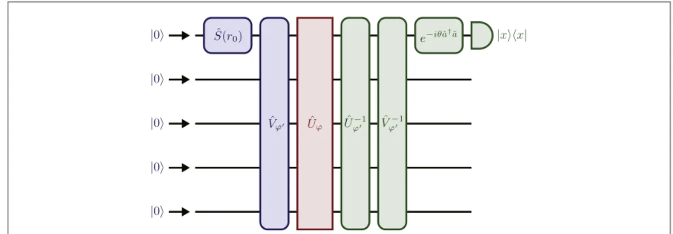
Another example of an optimal POVM can be obtained by considering the scheme depicted infigure2(the
circuit infigure2includes both the preparation stage for the optimal input state∣y ñopt in(3.31) and the probing stage together with the circuit Uˆj). The measurement is to first undo the circuit Uˆ as well as the transformationj Vˆ applied to prepare the optimal input statej ∣y ñopt in(3.31), and then to perform the homodyne measurement
on thefirst mode along the quadrature x e a axe a a x cos y sin 1 = i 1 1 1 i 1 1= 1 q+ 1 q
q q -q
ˆ( ) ˆ ˆ† ˆ ˆ ˆ† ˆ ˆ
withq = tan-1 2e r0.
Accordingly, the elements{ ˆ }Px of the POVM for this measurement can be expressed as
U V e x x e V U , 4.7
x ia a1 1 ia a1 1
^ ^ ^ ^ ^ ^ ^^ ^
P = j j q (∣ ⟩⟨ ∣Ä ÄÄ ) -q j† j† ( )
† †
where∣xñis the eigenvector of the quadrature operatorxˆ1such that x xˆ ∣1 ñ =x x∣ ñ, normalized as
x x d x x
á ∣ ¢ñ = ( - ¢). Indeed, the FI by this POVM{ ˆ }Px for the optimal input∣y ñopt in(3.31) coincides with the upper bound of the QFI in(1.4). See appendixDfor the proof. This is a generalization of the result given in[19],
from a single-mode phase shift to a generic multimode passive linear circuit.
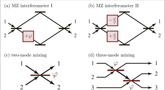
5. Simple examples
Let us look at a few simple examples, i.e.the two- and three-mode circuits shown in figure3, to see in particular how the unitary Vˆ involved in the optimal input Gaussian statej (3.31) looks like. The optimal input Gaussian states∣y ñopt and the maximal QFIs F( ∣∣j y ñopt )for those examples are summarized in table1.
Figure 2. An overall circuit to achieve the ultimate precision bound in(1.4), including the preparation stage for the optimal input
state∣y ñopt in(3.31) and the measurement stage, where x x∣ ñá ∣represents the homodyne measurement on thefirst mode along the
quadrature xˆ1=( ˆa1+aˆ )1† 2and the phase shiftθ is tuned toq = tan-1 2er0. Note thatj of Uˆ is the target parameter to bej estimated, which is not under our control, whilej¢ofVˆj¢,Uj¢1
-ˆ , andVj¢1
-ˆ is decided by ourselves. Tuningj¢to the true valuej provides us with the optimal strategy. The perfect cancellation of Uˆ byj Uj¢1
-ˆ tells us that our guessed valuej¢perfectly matches the
5.1. Mach-Zehnder(MZ) interferometer I
Wefirst consider the MZ interferometer in figure3(a). Our target is the phase shift j in one of the two arms of
the interferometer. The state of the probe photons going through this MZ interferometer is transformed by the unitary transformation U U e a aU , 5.1 12 4 i 1 1 12 4 = j
( )
p -j( )
p ˆ ˆ† ˆ ˆ† ˆ ( ) where Uˆmn( )q =eq( ˆ ˆa an m-a aˆ ˆ )m n (5.2) † †describes a beam splitter for modes m and n, which acts on the canonical operators as
U a U U a U a a U a a cos sin sin cos , 5.3 mn m mn mn n mn m n mn m n q q q q q q q q q = - = ⎛ ⎝ ⎜ ⎜ ⎞ ⎠ ⎟ ⎟
(
)
⎛⎝⎜ ⎞⎠⎟ ⎛⎝⎜ ⎞⎠⎟ ˆ ( ) ˆ ˆ ( ) ˆ ( ) ˆ ˆ ( ) ˆ ˆ ( ) ˆ ˆ ( ) † †withθ characterizing its transmissivity. In particular, Uˆmn 4
( )
p describes a balanced beam splitter. The generator of this two-mode circuit readsG iU dU U a a U
dj 12 4 1 1 12 4 . 5.4
= =
j j j
( )
p( )
pˆ ˆ† ˆ ˆ† ˆ ˆ ˆ† ( )
The unitary matrix Ujrelated to the unitary transformation Uˆ through(j 2.2) is given by
U U e 0 U 0 1 , 5.5 12 4 i 12 4 = j p j p -⎜ ⎟ ⎛ ⎝ ⎞⎠
( )
( )
( ) †Figure 3.(a)–(b) Two different arrangements of the MZ interferometer. (c) Two-mode mixing circuit. (d) Three-mode mixing circuit.
Table 1. The optimal Gaussian input state∣y ñopt and the maximal QFIF( ∣∣j y ñopt)for
the estimation of the parameterj in each of the circuits shown in figure3.
opt y ñ ∣ F( ∣∣j y ñopt ) MZ interferometer I U12 4 S r1 0 0ñ p
( )
ˆ† ˆ ( )∣ N N 8 ( +1) MZ interferometer II U12 4 S r1 0 0ñ p( )
ˆ† ˆ ( )∣ N N 2 ( +1) Two-mode mixing e a a a a U S r 0 12 4 1 0 i 4 1 1-2 2 p ñ p( )
ˆ ˆ ( )∣ ( ˆ ˆ† ˆ ˆ )† † 8N N( +1) Three-mode mixing U e a aU U S r 0 12 31 4 12 4 1 0 i 2 2 2 j p( ) ( )
p p ñ ˆ ( )† ˆ ˆ† ˆ ˆ ˆ ( )∣ N N 16 ( +1)and its generator reads g iU dU U U d 1 0 0 0 . 5.6 12 4 12 4 j = = j j† j †
( )
p( )
( )
p ( ) We thus have gj =1. 5.7 ( )The unitary operator Vˆ corresponding to the unitary matrix diagonalizing gj jin(5.6) (compare it with (A.23)) is
Vˆj=Uˆ12 4†
( )
p . (5.8)Therefore, the optimal Gaussian input state(3.31) for this MZ interferometer is given by
U S r 0 , 5.9
opt 12 4 1 0
y ñ =
( )
p ñ∣ ˆ† ˆ ( )∣ ( )
with the squeezing parameter r0given in(3.30). By this choice, the QFI reaches the upper bound in(1.4), yielding
F( ∣∣j y ñ =opt ) 8N N( +1 .) (5.10)
Notice that, in this case, the optimal input state∣y ñopt in(5.9) is independent of the target parameter j. Note also that the same expression as(5.10) is found e.g.in [14,19,34,40,59], but it is found there as the optimal QFI
for the estimation of the single-mode phase shift with a Gaussian probe. Here,(5.10) is presented as the optimal
QFI for the two-mode circuit infigure3(a).
The unitary transformation Uˆ12 4†
( )
p in the optimal input state(5.9) ‘unfolds’ the first beam splitter Uˆ12 4( )
p of the MZ interferometer. Thus, the best strategy effectively consists in sending the single-mode squeezed vacuumr0ñ =S r1 0 0ñ
∣ ˆ ( )∣ directly to the phase shifter without thefirst beam splitter Uˆ12 4
( )
p . The second beam splitter Uˆ12 4†( )
p of the MZ interferometer is also unfolded by Uˆ12 4( )
p performed in the optimal measurements(see (4.4)and(4.7),where Uˆ contains Uj ˆ12 4†
( )
p , whose Hermitian conjugate Uˆ12 4( )
p in Uˆj †acts on the output probe state first in the measurement process, canceling the second beam splitter Uˆ12 4†
( )
p ).5.2. MZ interferometer II
Let us look at the MZ interferometer in the slightly different configuration shown in figure3(b). This setup
induces the unitary transformation
U U e a a a a U , 5.11 12 4 i2 1 1 2 2 12 4 = j p - - p j
( )
( )
ˆ ˆ† ( ˆ ˆ† ˆ ˆ )† ˆ ( )and its generator is given by
G 1U a a a a U
2 12 4 1 1 2 2 12 4 . 5.12
=
-j
( )
p( )
pˆ ˆ† ( ˆ ˆ† ˆ ˆ ) ˆ† ( )
The unitary matrix Ujcorresponding to the unitary operator Uˆ inj (5.11) is given by
U U e 0 U 0 e , 5.13 12 4 i 2 i 2 12 4 = j p j j p -⎛ ⎝ ⎜ ⎞ ⎠ ⎟
( )
( )
( ) †while the Hermitian matrix gjcorresponding to the generatorGˆjin(5.12) reads
g U 1 2 0 U 0 1 2 . 5.14 12 4 12 4 = -j p p ⎛ ⎝ ⎜ ⎞⎠⎟
( )
( )
( ) † / / We thus have g 1 2. 5.15 = j ( )The optimal Gaussian input state for this MZ interferometer is the same as the one given in(5.9), while the
maximal QFI achievable by the optimal input state is
F( ∣∣j y ñ =opt ) 2N N( +1 .) (5.16)
This QFI is lower than the previous one in(5.10) for the other MZ interferometer, even though the relative
phasesj to be estimated in the two MZ interferometers are the same. This is because injecting all the resources to one of the two arms of the interferometer is optimal if we stick to Gaussian probes, and only one of the two phase shifters infigure3(b) is probed. It would be worth noticing that our estimation problem implicitly assumes the
and(b) are equivalent, since only the relative phase between the two arms matters in such a case. See the discussion in[26].
5.3. Two-mode mixing
Let us look at another two-mode example: the estimation of the parameterj characterizing the transmissivity of the beam splitter represented by the unitary transformation
Uˆj=Uˆ ( )12 j. (5.17)
Seefigure3(c). Its generator reads
Gˆj=i( ˆ ˆa a2 1† -a aˆ ˆ )1† 2 , (5.18) which can be rewritten as
G e a a a a U a a a a U e a a a a . 5.19 12 4 1 1 2 2 12 4 i 4 1 1 2 2 4i 1 1 2 2 = -j p -
( )
p( )
p -p -ˆ ( ˆ ˆ† ˆ ˆ )† ˆ† ( ˆ ˆ† ˆ ˆ ) ˆ† ( ˆ ˆ† ˆ ˆ )† ( )It is unitarily equivalent to the generatorGˆjin(5.12), apart from the numerical proportionality constant 1/2. We thus have
gj =1, 5.20
( )
and the maximal QFI is given by
F( ∣∣j y ñ =opt ) 8N N( +1 .) (5.21)
This is reached by the input state
U S r e a a a a 0 , 5.22 opt 12 4 1 0 i 4 1 1 2 2 y ñ = p - p ñ
( )
∣ ( ˆ ˆ† ˆ ˆ )† ˆ† ˆ ( )∣ ( )with the squeezing parameter r0given in(3.30). This optimal state is again independent of the target parameterj.
The same estimation problem, i.e.the estimation of j in the two-mode mixing channel (5.17), is studied in
[59], but the maximal QFI (5.21) and the optimal Gaussian input state (5.22) are not identified there.
5.4. Three-mode mixing
Let us also look at a three-mode example. We consider the circuit shown infigure3(d), composed of two beam
splitters of the same transmissivity characterized by the parameterj. Our problem is to estimate the single parameterj in the three-mode mixing circuit represented by the unitary transformation
Uˆj=Uˆ ( ) ˆ ( )23 j U12 j. (5.23)
Its generator reads
G U a a a a a a a a U V a a a a V i 2 , 5.24 12 3 2 2 3 2 1 1 2 12 1 1 2 2 j j = - + -= -j j j ˆ ˆ ( )( ˆ ˆ ˆ ˆ ˆ ˆ ˆ ˆ ) ˆ ( ) ˆ ( ˆ ˆ ˆ ˆ ) ˆ ( ) † † † † † † † † with V U e a aU U . 5.25 12 31 4 12 4 i 2 2 2 j = j p
( ) ( )
p p ˆ ˆ ( )† ˆ ˆ† ˆ ˆ ( ) We have gj = 2 , 5.26 ( )and the maximal QFI is given by
F( ∣∣j y ñ =opt ) 16N N( +1 .) (5.27)
This is reached by the input state
U e a aU U S r 0 , 5.28 opt 12 31 4 12 4 1 0 i 2 2 2 y ñ = j p p p ñ
( ) ( )
∣ ˆ ( )† ˆ ˆ† ˆ ˆ ˆ ( )∣ ( )with the squeezing parameter r0given in(3.30). In this case, the optimal input state depends on the target parameterj.
If our guessj¢is not precise and does not match the true valuej, the input state (3.31) and the
measurement, e.g.(4.6) or (4.7), prepared and performed with the guessed valuej¢in place ofj (see e.g. the circuit infigure2) are not optimal, and the FI for such a nonoptimal probing deviates from the maximal QFI
in(1.4). Since we assume that the functional dependence of Ujˆ uponj is smooth, the FI is a smooth function of
j¢, and therefore, the deviation of FI from the maximal QFI is only quadratic around the optimal point j¢ = .j In this sense, the FI is robust to a small error in the guess ofj.
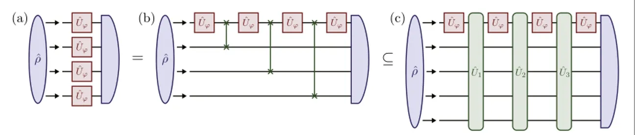
6. Sequential strategy
If we are allowed to use multiple(identical) target circuits Uˆ at the same time, we could do better. Suppose thatj we are given L identical M-mode passive linear circuits Uˆ . A paradigmatic scheme for the quantum metrology isj the parallel scheme infigure4(a) with an entangled inputrˆ[2,4]. The result in section3suggests, however, that, if we stick to Gaussian inputs, this parallel setup does not help improve the maximal QFI found in(1.4), since the
best strategy is to inject all the resources into a single-mode of the overall LM-mode passive linear circuit in figure4(a): only one of the L circuits is probed with the others irrelevant. See(3.31). On the other hand, if we are
allowed to perform some operations U{ ˆ1,¼,UˆL-1}between the target gates Uˆ with ancilla modes introducedj as infigure4(c), we can hope to do better. Let us restrict ourselves to passive linear controls U{ ˆ1,¼,UˆL-1}, and seek for the optimal strategy with a Gaussian inputr Έ (K N, ), whereKLM.
The circuit infigure4(c) is described by the unitary
U UL 1U U U U U .2 1 6.1
=ˆj ˆ ˆj - ˆj ˆ ˆ ˆ ˆj j ( )
Note that there are K(LM)modes in total in the overall circuit, and the unitary operators Uˆ act only on thej first M modes, i.e.UˆjÄ. By abuse of notation, UˆjÄis simply denoted by Uˆ in(j 6.1). The overall circuit is a K-mode passive linear circuit, and the orthogonal matrix jwhich rotates the quadrature operatorszˆin phase space according to the transformationˆjis given by
W 0 W 0 * 6.2 = j j j ⎛ ⎝ ⎜⎜ ⎞⎠⎟⎟ ( ) † with U UL 1U U U U U ,2 1 6.3 =j j - j j j ( )
where Ujand Uℓ(ℓ=1,¼,L-1) are K×K unitary matrices corresponding to UˆjÄand Uˆℓ, respectively. The quantity relevant to the maximal QFI is the spectral norm of the generator of this orthogonal transformation j(see (1.4)), i.e.the largest (in magnitude) eigenvalue of
U U U U g U U U U i d d , 6.4 L 0 1 1 1
å
j = = j j j j j j j j = - ( ) ℓ ℓ ℓ † † † † † where g iU dU dj . 6.5 = j j† j ( )The spectral norm of the generatorjis bounded from above as
U U U U g U U U U U U U U g U U U U L g . 6.6 L L 0 1 1 1 0 1 1 1
å
å
= = j j j j j j j j j j j j = -= - - ( ) ℓ ℓ ℓ ℓ ℓ ℓ † † † † † † † †This inequality is saturated if
gj,U Uj =0 ℓ=1,¼,L-1 . 6.7
[ ℓ ] ( ) ( )
A sufficient and general solution is given by
Uℓ=Uj† (ℓ=1,¼,L-1) (6.8)
Figure 4. The parallel scheme in(a) is equivalent to the sequential scheme in (b) with the target circuits Uˆ swapped byj SWAPgates, which is a particular case of the sequential scheme in(c) with generic gates Uˆℓentangling the main probes with additional ancillas.
(see [95]). By this choice, the generator of the overall circuitˆjis reduced to =j Lgj, and the upper bound on the QFI by the sequential strategy with a Gaussian inputr Έ (K N, )is given by
L g N N
8 2 2 1 . 6.9
( ∣ ˆ )j r j ( + ) ( )
This upper bound is saturated by the input state
0 , 6.10
opt yopt
Y ñ = ñ Ä ñ
∣ ∣ ∣ ( )
with∣y ñopt given in(3.31) for the first M modes while vacuum for the rest.
The results in(6.8) and(6.10) show that the ancilla modes are not necessary for the optimal strategy. We
note that in general the optimal controls(6.8) and the optimal input state(6.10) depend on the target
parameterj.
7. Summary
We have clarified the universal bound(1.4) on the precision of the estimation (QFI) of a parameter embedded in
a generic multimode passive(photon number preserving) linear optical circuit by using Gaussian probes with a given average number of probe photonsN. We have identified the input Gaussian state(3.31) that yields the
QFI saturating the bound(1.4): it is a single-mode squeezed vacuum in an appropriate basis. We have also found
measurements(POVMs)(4.6) and(4.7) by which FI reaches QFI. The best (sequential) strategy when we are
given multiple identical target circuits and are allowed to apply passive linear controls in between with the help of an arbitrary number of ancilla modes has been revealed: no ancilla mode is actually needed for the best strategy6.
Even though the optimal input state(3.31) and the optimal measurements(4.6) and(4.7), as well as the
optimal controls(6.8) in the sequential strategy, depend on the target parameter to be estimated in general and
adaptive adjustments of the input, the measurement, and the controls would be required to achieve the precision bound in practice, the above result shows that the bound is sharp and covers various specific setups composed of phase shifters and beam splitters, including the standard MZ interferometer, providing the universal bound that cannot be beaten by any Gaussian inputs and any passive controls.
The present work has focussed on passive linear circuits. Bounds on more general Gaussian metrology, for general Gaussian channels including amplitude-damping channels and channels involving squeezing, etc., have not been thoroughly understood yet, beyond analyses on specific setups. Entanglement with ancilla modes would be useful for such generic Gaussian metrology[17] and it would be interesting to explore.
Acknowledgments
KY thanks Koji Matsuoka for the discussions during his master’s thesis study [98], in which the bound (1.4) and
the optimal input state(3.31) were found for some restricted setups. This work was supported by the Top Global
University Project from the Ministry of Education, Culture, Sports, Science and Technology(MEXT), Japan. KY was supported by the Grant-in-Aid for Scientific Research (C) (No.18K03470) from the Japan Society for the Promotion of Science(JSPS) and by the Waseda University Grant for Special Research Projects (No. 2018K-262). PF was supported by INFN through the project ‘QUANTUM,’ and by the Italian National Group of Mathematical Physics(GNFM-INdAM).
Appendix A. Gaussian states and operations
In order to introduce a proper definition of the Gaussian set M N( , ), wefind it useful to introduce the quadrature operators xˆmand yˆmfor each of the M modes,
x y m 1, ,M . A.1 m a a m a a 2 2 i m m m m ^ ^ ^ ^ ^ ^ = = = ¼ + -⎧ ⎨ ⎪ ⎩ ⎪ ( ) ( ) † † 6
There are works in the literature which discuss the unnecessity of mode entanglement[5,39,40,50,53,55,96,97]. Note, however, that in
those works the probe states are not restricted to Gaussian states and in addition just the achievability of the Heisenberg scaling(quadratic in
N) is discussed. The chosen probe states are not necessarily the optimal ones, even though they actually yields QFIs scaling quadratically in N(their coefficients are not necessarily the optimal). On the other hand, in the present work, we look at the optimal state which yields the
Aligning these operators as a column vector z x y x x y y , A.2 M M 1 1 = = ⎛ ⎝ ⎜ ⎞⎠⎟ ⎛ ⎝ ⎜ ⎜ ⎜ ⎜ ⎜ ⎜⎜ ⎞ ⎠ ⎟ ⎟ ⎟ ⎟ ⎟ ⎟⎟ ˆ ˆ ˆ ˆ ˆ ˆ ˆ ( )
the above relation(A.1) can be expressed as
a a x y W A.3 = ⎜ ⎟ ⎛ ⎝ ⎞ ⎠ ⎛ ⎝ ⎜ ⎞ ⎠ ⎟ ˆ ˆ ˆ ˆ ( ) †
with a M2 ´2Munitary matrix
W 1 2 i i . A.4 =
-(
)
( )The canonical commutation relations(2.1) can then be expressed in the compact form
zm,zn =iJmn m n, =1,¼, 2M , A.5
[ ˆ ˆ ] ( ) ( )
with Jbeing the M2 ´2Mreal matrix
J 0 0 . A.6 =
-(
)
( )A.1. Gaussian states
A Gaussian staterˆis fully characterized by its covariance matrixΓ and its displacement d, defined by
z z z z d z m n M
1
2 , , , 1, , 2 , A.7
mn m n m n m m
G = á{ˆ ˆ }ñ - á ñá ñˆ ˆ = á ñˆ ( = ¼ ) ( )
where á denotes the expectation value onñ rˆ. In particular, its characteristic function reads as
ei z e 1 T i d. A.8
2
h
c( )= á h· ˆñ = - h G +h h· ( )
Furthermore,rˆis an element of(M N, )when its mean photon number is equal toN, i.e.
d N 1 N 2 Tr 1 2 , A.9 2 á ñ = ⎡ ⎜G - ⎟+ = ⎣⎢ ⎛ ⎝ ⎞⎠ ⎤ ⎦⎥ ˆ ( )
where the number operatorNˆis defined in(2.3). The covariance matrix Γ is real, symmetric, and
positive-definite, and hence, according to Williamson’s theorem it admits the canonical decomposition [83,84]
RQR R QR ,T T A.10 G = ¢S ¢ ( ) where Q 0 0 , e 0 0 e , A.11 r r s s S =
(
)
=(
-)
( ) R W U U W R W U U W 0 0 , 0 0 , A.12 * * = ¢ = ¢ ¢ ⎜ ⎟ ⎜ ⎟ ⎛ ⎝ ⎞⎠ ⎛ ⎝ ⎞ ⎠ ( ) † †with M×M diagonal submatrices
r r r , , A.13 M M 1 1 s s s =⎛ = ⎝ ⎜⎜ ⎞⎠⎟⎟ ⎛⎝⎜⎜ ⎞⎠⎟⎟ ( )
and M×M unitary submatrices U and U¢7
. The M2 ´2Mmatrices R andR¢are real orthogonal matrices, and we have RT =R†=R-1and R¢ = ¢ = ¢T R† R-1. The parameters , ,
M 1
s ¼ s
{ }are the symplectic eigenvalues of Γ, which control the purity p r( ˆ )of the Gaussian staterˆthrough[84]
7Note that U*is not the Hermitian conjugateU†of the M×M matrix U, but is obtained by taking the complex conjugate of each matrix
element of U. In other words, it is U*=(U†)T=(UT)†, with T denoting the matrix transpose. This U*is necessary in the structure of R in
p Tr 1 det 2 1 2 , A.14 m M m 2 1
r r s = = G = = ( ˆ ) ˆ ( ) ( )while r{1,¼,rM}are the squeezing parameters. The symplectic eigenvalues are bounded from below by 1 2
m
s (m=1, K, M) due to the uncertainty principle [83,84]. The Gaussian staterˆis pure, p( ˆ )r =1, if and only if all the symplectic eigenvalues saturate the lower boundss =m 1 2(m=1, K, M). Without loss of generality, we assume that
r r r 1 2, 0. A.15 M M 1 2 1 2 s s s ( )
This reordering can always be done by arranging properly R andR¢. The matrices R andR¢are symplectic and orthogonal, characterized by the structure(A.12) with the unitary matrices U and U¢. The squeezing matrix Q is
also symplectic. The symplectic character of these matrices is characterized by
R JRT =J, R JR¢T ¢ =J, Q JQT =J. (A.16)
A.2.M-mode passive Gaussian unitary
Our target circuit Uˆ is a generic M-mode passive Gaussian unitary, whose action is characterized by the M×Mj unitary matrix Ujintroduced in(2.2). In terms of the quadrature operators zmˆ , it is rephrased as
U z Um R z m 1, , 2M , A.17 n M mn n 1 2
å
= = ¼ j j j = ˆ ˆ ˆ† ( ) ˆ ( ) ( )or simply written asUˆ ˆ ˆj†zUj=Rjzˆ, with Rjbeing the M2 ´2Morthogonal matrix defined by
R W U U W 0 0 * . A.18 = j j j ⎛ ⎝ ⎜⎜ ⎞⎠⎟⎟ ( ) †
As is clear from this structure, the matrix Rjis symplectic and orthogonal, and the passive linear transformation Uˆ is a rotation on the phase space.j
By construction the transformation Uˆ maps the setj (M N, )into itself. In particular, givenr Έ (M N, ), the covariance matrix Gjand the displacement djof the associated Gaussian output staterˆjin(1.1) are obtained by rotating the covariance matrixΓ and the displacement d of the input staterˆas
d d
R RT, R . A.19
G =j jG j j= j ( )
Note that they still fulfill the constraint(A.9) due to the fact that Rjis orthogonal.
An important role on our problem is played by the generator of the transformation Ujˆ , i.e.by the operator
G iU dU
dj , A.20
=
j j j
ˆ ˆ† ˆ ( )
whose equivalent on the phase space reads
G R R W g g W i d d 0 0 A.21 T * j = = -j j j j j ⎛ ⎝ ⎜⎜ ⎞⎠⎟⎟ ( ) † with g iU dU dj . A.22 = j j† j ( )
This gjis an M×M Hermitian matrix, that can be diagonalized by means of an M×M unitary matrix Vj,
g V V , , A.23 M 1 e e e e = = j j j j j ⎛ ⎝ ⎜⎜ ⎞⎠⎟⎟ ( ) †
where, without loss of generality, the magnitudes of the eigenvaluese of gm jare ordered in decreasing order
. A.24
M 1 2
e e e
∣ ∣ ∣ ∣ ∣ ∣ ( )
The generator Gjis accordingly diagonalized as
G P W 0 WP P J P 0 i , A.25 T T e e = - = j j j j j j j j ⎛ ⎝ ⎜ ⎞ ⎠ ⎟ ( ) ( ) †
where P W V V W 0 0 , 0 0 . A.26 * e e = = j j j j j j ⎛ ⎝ ⎜⎜ ⎞ ⎠ ⎟⎟ ⎛⎝⎜ ⎞⎠⎟ ( ) †
Appendix B. Derivation of the expression
(
3.17
) for
F
( )1( ∣ )
j r
^
Here, we show the derivation of the expression for F( )1( ∣ ˆ )j r in(3.17). Notice first that R in (A.12) is a real matrix, and hence,
R R R W U U W 0 0 . B.1 T T 1 = = - = ⎛ ⎝ ⎜ ⎞⎠⎟ ( ) † † †
Inserting this into(3.9), the covariance matrix Γ of a pure Gaussian state is expressed as
W U U W W U U W W U r U U r U U r U U r U W 1 2 0 0 e 0 0 e 0 0 1 2 cosh 2 sinh 2 sinh 2 cosh 2 , B.2 r r T T T 2 2 G = = * -* * ⎛ ⎝ ⎜ ⎞ ⎠ ⎟ ⎛ ⎝ ⎜ ⎞⎠⎟ ⎛ ⎝ ⎜ ⎞⎠⎟
(
)
( ) † † † † † † and we have W U r U U r U U r U U r U W 2 cosh 2 sinh 2 sinh 2 cosh 2 . B.3 T T 1 * * G = -- ⎛ ⎝ ⎜ ⎞ ⎠ ⎟ ( ) † † † Then, inserting these and(A.21) into the first line of (3.17), we getF G G G U g U r r U g U U g U r U g U r g g 1 2Tr 1 2Tr cosh 2 1 2Tr cosh 2 Tr sinh 2 sinh 2 1 2Tr 1 2Tr . B.4 T T 1 1 2 2 2 2 2 * * * * * j r = G G -= + + - -j j j j j j j j j -( ∣ ˆ ) ( ) [( ) ] [( ) ] ( ) ( ) ( ) ( ) ( ) † †
Since gjis Hermitian and hence gj* =gjT, this is simplified to the expression in (3.17), notingTr(AT)=TrAfor any matrix A.
Appendix C. Some useful inequalities
Lemma 1. For Hermitian matrices A and B,
AB A B
Tr[( ) ]2 Tr( 2 2). (C.1)
The equality holds if and only if[A B, ]=0. Proof. Since ABi( -BA)is Hermitian,
AB BA AB A B 0 Tr i 2 Tr 2 Tr . C.2 2 2 2 2 -= - + {[ ( )] } [( ) ] ( ) ( )
Therefore, the inequality(C.1) follows. The equality holds if and only if AB-BA= .0 ,
Lemma 2. For Hermitian matrices A and B,
A B AB A B
Tr( T T )Tr( 2 2). (C.3)
The equality holds if and only if AB= (AB)T. Proof. By noting the Hermitianity of A and B,
AB AB AB AB A B A B AB 0 Tr 2 Tr 2 Tr . C.4 T T T T 2 2 - -= -{[ ( ) ] [ ( ) ]} ( ) ( ) ( ) †