Optimization of drying food products: application to fruits

Sapienza Università di Roma

Dipartimento Ingegneria Chimica Materiali ed Ambiente

OPTIMIZATION OF DRYING FOOD PRODUCTS:

APPLICATION TO FRUITS

PhD in Chemical Engineering

XXX cycle

Tutor Candidate

Prof.ssa Paola Russo Renato Buonocore

Acknowledgements

I would like to express my acknowledgements for the support in the experimental work to the team of the Laboratorio di Tecnologie Alimentari, Dipartimento Ingegneria Industriale, Università di Salerno and the Laboratorio di Risonanza magnetica “Annalaura Segre”, Istituto di Metodologie Chimiche, CNR.

Abstract

Air drying is one of the most used unit operation in food processing. Simulation or designing the air-drying operation requires the mathematical description of food moisture evolution during the process, known as drying kinetics. The structure of the food materials goes through deformations due to the simultaneous effect of heat and mass transfer during the drying process. These deformations lead to changes in many quality attributes and directly affect physical properties (i.e. the mass diffusion coefficient). Changes in volume, “shrinkage”, negatively impact the quality perception of dried products by consumer. The knowledge of the changes in the properties of foods that occur during drying is hence needed for better designing the process.

The aim of this study is to understand the effect of drying on quality of fruit which typically has high moisture content (i.e. pear and grape) and to develop a mathematical model which quantify the drying of this food matrix. To this purpose the drying kinetics, shrinkage and structure modifications (through SEM analysis) were experimentally evaluated.

During drying, the macroscopic transport of water through the cellular tissue constituting the fruit is largely controlled by the microscopic distribution of water and air on a cellular and subcellular distance scale and by membranes permeability. 1H pulsed low resolution NMR allows to obtain quantitative information on water distribution and diffusion by detecting the proton signal predominantly due to H2O contained in vegetable tissue. Therefore, portable-NMR was used to determine the drying moisture profile and thickness reduction of pears. Portable-NMR also allowed to investigate water mobility in fresh and dried pears by measuring the longitudinal and transverse relaxation times, and the self-diffusion coefficient. For fruit, such as grape, drying is a slow and very energy intensive process because the waxy peel has low permeability to moisture. In order to enhance the drying rate, pretreatments are used. In this thesis, both chemical (by dipping in an ethyl oleate solution) and physical (by abrasion) pretreatments were analysed. It was found that ethyl oleate and abrasion pretreatments have the same effect in reducing the drying time, but the second one is to be preferred because it avoids the use of chemical additives and permits safer raisin to be produced. Moreover, the samples pretreated by peel abrasion showed less shrinkage and no cracks on the peel surface with respect to those pretreated with ethyl oleate solution.

To obtain a detailed prediction of moisture distribution during drying, in the thesis, a diffusion model with Fickian moisture transfer was coupled with an empirical law which considers the

is used with an adaptive mesh. The results match well with the experimental results. In particular, a good agreement between experimental and theoretical data of moisture ratio during drying was found for both fruits. The model also well predicted the moisture profile along the pear thickness obtained by NMR.

Contents

Acknowledgement ii

Abstract iii

List of Figures viii

List of Tables xiii

CHAPTER 1

Drying of fruit and vegetables

1 Introduction 1

1.1 Major approaches in drying modelling process of fruit and vegetables 3

1.2 Drying models 4

1.2.1 Empirical models 4

1.2.2 Models considering heat and mass transfer 6

1.2.3 Models considering shrinkage 10

1.3 Techniques for quality analysis of fruit and vegetable 17

1.3.1 Basic theory of NMR and MRI 17

1.3.2 NMR applied to fruit and vegetables 20

1.4 Thesis Objectives 28

1.5 Thesis Structures 29

CHAPTER 2

Pear experiment measurement

2 Material and methods 30

2.1 Sample preparation 30

2.2 Results 31

2.2.1 Drying experiments 31

2.2.2 Thickness reduction measure 35

2.3 NMR relaxometry 38

2.3.1 NMR data processing 39

2.3.2 1H NMR depth profiles 39

2.3.5 Self Diffusion coefficient 49

2.4 SEM images 52

2.5 Conclusion 54

CHAPTER 3

Modelling of pear drying

3 Analytical solution of Fick’s second low of diffusion 55

3.1 Drying kinetics 57

3.1.1 Moisture profile along z-axis 66

3.2 Mathematical modelling with shrinkage effect 70 3.3 Result of the model considering shrinkage 75

3.3.1 Drying kinetics 75

3.3.2 Predicted Mt/M0 profile along z-axis 77

3.4 Conclusion 79

CHAPTER 4

Drying of grapes

4 Introduction 80

4.1 Effect of physical pretreatment process on the drying kinetics 80

4.2 Materials and methods 89

4.2.1 Sample preparation 89

4.3 Results 90

4.3.1 Drying experiments 90

4.3.2 Shrinkage measurements 92

4.4 SEM images 97

4.5 Modelling of grape drying 99

4.5.1 Model in cylindrical and spherical coordinate 99 4.5.2 Results of the model in cylindrical coordinate 102 4.5.3 Results of the model in spherical coordinate 106

CHAPTER 5

Conclusions and future works 114

References

116

List of Figures

CHAPTER 1

Fig. 1. a) Experimental measurements fitted with model considering shrinkage for potato, b) linear fitting of change in radius vs. moisture content (Aprajeeta et al., 2005). 12 Fig. 2. Volume of potato slab vs moisture content for different air temperatures (Hassini et al.,

2007). 13

Fig. 3. Dimensionless free moisture content as a function of drying time (Barcelos et al.,

2011). 15

Fig. 4. Dimensionless free moisture content as a function of dimensionless radius at a given

drying time (Barcelos et al., 2011). 15

Fig. 5. Experimental and predicted total dimensionless water content temporal profiles during eggplant drying at different temperatures (Brasiello et al., 2013). 16 Fig. 6. Comparison of the MRI derived moisture spatial profiles during the dehydration of a

cylindrical sample of eggplant at 323 K with: (a) numerical data; (b) numerical data derived from Fick's model (Brasiello et al., 2017). 16 Fig. 7. Distribution of transverse water proton relaxation times in fresh ‘Red Delicious’ apple

tissue measured at spectrometer frequency of 23.4MHz with a CPMG 90–180◦ pulse spacing of 200s. Numbers refers to relaxation peaks of the water proton in the different cell compartments: 1, the vacuole; 2 and 3, cytoplasm and extra-cellular compartment and 4, cell wall (Maringheto et al., 2008). 21 Fig. 8. Sketch of the geometry of the magnet of the profile NMR mouse. 21 Fig. 9. Measurement of intact kiwifruit with a single-sided NMR sensor (Capitani et al., 2010).

22 Fig. 10. Transverse relaxation times distribution measured on ripened kiwifruit (Capitani et al.,

2010). 22

Fig. 11. Measurement in field on entire kiwifruit attached to the tree with a portable unilateral

NMR instrument (Capitani et al., 2013). 23

Fig. 12. Transverse relaxation curves measured in field in October, November, and December on Hayward (a), CI.GI (b), and Zespri (c) with the corresponding relaxation time

Fig. 14. T2 distributions of three fresh blueberries, and the same blueberries let to wither for three days, and for six days (Capitani et al., 2014). 25 Fig. 15. Two-dimensional spin echo images of eggplant at 50 and 60°C and selected drying

times (Adiletta et al., 2013). 26

Fig. 16. Moisture ratio (%) of samples during drying obtained by gravimetric method and MRI at T = 50 °C (a) and 60 °C (b) (Adiletta et al., 2014). 37 Fig. 17. Experimental shrinkage data and prediction by power model (Adiletta et al., 2014).

27

CHAPTER 2

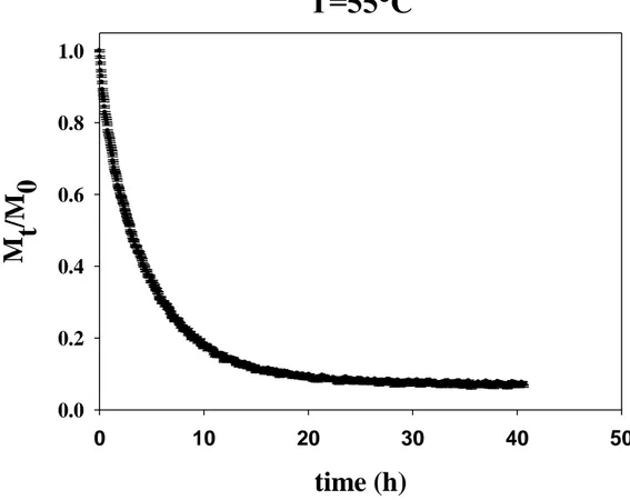
Fig. 18. Parallelepiped sample of fresh pear. 30 Fig. 19. Convective oven (air velocity of 2.3 m/s) used for the experiments. 31 Fig. 20. Weight sensor on which there is a perforated network where lie the sample. 32 Fig. 21. Moisture ratio of spherical pear sample during drying at T=45°C. 32 Fig. 22. Moisture ratio of spherical pear sample during drying at T=50°C. 33 Fig. 23. Moisture ratio of spherical pear sample during drying at T=55°C. 33 Fig. 24. Moisture ratio of parallelepiped pear sample during drying at T=45°C. 34 Fig. 25. Moisture ratio of parallelepiped pear sample during drying at T=50°C. 34 Fig. 26. Moisture ratio of parallelepiped pear sample during drying at T=55°C. 35 Fig. 27. Experimental data of average thickness reduction L/L0 vs Mt/M0 36

Fig. 28.a) Linear relationship obtained by NMR and vernier caliper measurements at T=50°C, b) thickness reduction obtained by NMR at 45, 50 and 55°C. 37 Fig. 29. Direction of the magnetic field. 40 Fig. 30. Depth profiles of fresh and dried pear samples for 3, 6, 15, 20, 29, 48 at (a) 45, (b) 50

and (c) 55°C. 41

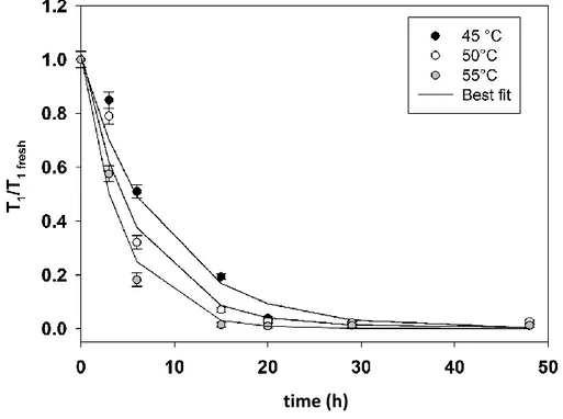
Fig. 31. Variation of moisture content (It/I0) measured by NMR (a), relationship between NMR integral ratio It/I0 and Mt/M0 at (b) 45°C, (c) 50°C and (d) 55°C. 43 Fig. 32. T1 /T1fresh of pear samples at different drying time at 45, 50 and 55°C and best fit.

44 Fig. 33. T2 values of fresh pear samples in homogeneous (a) and not homogeneous field

NMR (b). 46

Fig. 34. T2 distribution at (a) 45°C, (b) 50 °C and (c) 55°C at 1 mm of depth, T2 distribution at (d) 45°C, (e) 50 °C and (f) 55°C at 5 mm of depth. 47 Fig. 35. Loss of population associated to water in the vacuole as a function of the drying time

Fig. 36. Dependence of echo attenuation (At) on the self-diffusion coefficient and relaxation

time at 45, 50 and 55°C. 50

Fig. 37. SEM images of pear sample at: 45 °C after a) 15 h, b) 20 h, c)29 h, d) 48 h; 50 °C after e) 15 h, f) 20 h, g)29 h, h) 48 h ; 55 °C after i) 15 h, l) 20 h, m)29 h, n) 48 h.

53

CHAPTER 3

Fig. 38. Experimental and predicted total dimensionless water content vs time at T=45°C and

the residual for spherical pear sample. 59

Fig. 39. Experimental and predicted total dimensionless water content vs time at T=50°C

and the residual for spherical pear sample. 60

Fig. 40. Experimental and predicted total dimensionless water content vs time at T=55°C and

the residual for spherical pear sample. 61

Fig. 41. Experimental and predicted total dimensionless water content vs time at T=45°C and

the residual for cubical pear sample. 63

Fig. 42. Experimental and predicted total dimensionless water content vs time at T=50°C and

the residual for cubical pear sample. 64

Fig. 43. Experimental and predicted total dimensionless water content vs time at T=55°C and

the residual for cubical pear sample. 65

Fig. 44. Predicted concentration distribution at various times in a spherical pear sample at

T=45°C. 66

Fig. 45. Predicted concentration distribution at various times in a spherical pear sample at

T=50°C. 67

Fig. 46. Predicted concentration distribution at various times in a spherical pear sample at

T=55°C. 67

Fig. 47. Predicted concentration distribution at various times in a cubical pear sample at

T=45°C. 68

Fig. 48. Predicted concentration distribution at various times in a cubical pear sample at

T=50 °C. 68

Fig. 49. Predicted concentration distribution at various times in a cubical pear sample at

T=55°C. 69

Fig. 53. Evolution of the mesh for 1/8 of parallelepiped during simulation. 74 Fig. 54. Moisture ratio during drying at fixed hm and different value of Deff (a); at fixed Deff

and different value of hm (b) for T=50°C. 75

Fig. 55. Moisture ratio of parallelepiped pear samples during drying at (a) 45, (b) 50 and (c)

55°C. 76

Fig. 56. Comparison of depth profile of fresh and dried pear obtained with NMR with simulated Mt/M0 profile along z-axis, at (a) 45, (b) 50 and (c) 55°C. 78

CHAPTER 4

Fig. 57. Experimental values of humidity (% dry matter) vs drying time for grape berries the peel of which was untreated (UTR) or pre-treated by dipping into ethyl oleate (EtOl)

or by abrasion (Abr) (Di Matteo et al., 2000). 81

Fig. 58. Schematic diagram of water (or steam) concentration profiles in the grape pulp and peel, and in the gaseous film surrounding each grape berry (Di Matteo et al., 2000).

82 Fig. 59. Experimental (Sp), and theoretical (Th) values of moisture changes (%) vs. drying

time for plums, the peel of which was untreated (UT) or pre-treated by dipping into ethyl oleate (EtOl) or by abrasion (Abr) (Di Matteo et al., 2002). 86 Fig. 60. Variation of moisture ratio with drying time (s) under different conditions, 50°C (

); ethyl oleate emulsion, 50°C ( ), 60°C ( ), ethyl oleate emulsion, 70°C (---)

(Esmaiili et al., 2007). 87

Fig. 61. Variation of effective diffusivity (m2_s-1_{) with moisture content (g/g}

d.b.) of the ethyl oleate emulsion and hot water-pretreated grapes at different temperatures; hot water, 50°C ( ); ethyl oleate emulsion, 50°C ( ); ethyl oleate emulsion, 60°C ( ); ethyl oleate emulsion, 70°C ( ) (Esmaiili et al., 2007). 88 Fig. 62. Experimental (symbols) and predicted (lines) drying curves of untreated (UTR) and

pretreated (TR-ABR, TR-EtOl) samples at 50 °C (Adiletta et al., 2016). 89 Fig. 63. Experimental data (symbols) and prediction (curves) of volume shrinkage of grape

during drying at 50 °C (Adiletta et al., 2016) 89

Fig. 64. Experimental moisture ratio vs time of (a) untreated UTR, (b) pretreated TR-Abr, (c)

TR-EtOl grape at 50, 60 and 70 °C. 92

Fig. 66. Experimental average diameter reduction Dt/D0 vs Mt/M0 for (a) UTR, (b) TR-Abr,

(c) TR-EtOl at 50, 60 and 70°C. 96

Fig. 67. SEM images of peel for: (a) fresh untreated sample, (b) fresh abraded sample, (c) fresh sample dipped in ethyl oleate solution and for dried sample at 50 °C: (d) untreated, (e) pretreated by abrasion and (f) preteated by ethyl oleate. 98 Fig. 68. Initial mesh for (a) cylinder and (b) sphere. 101 Fig. 69. Moisture ratio during drying at fixed hm and different value of Deff (a); at fixed Deff

and different value of hm (b) for TR-Abr=50°C. 102

Fig. 70. Experimental and predicted moisture ratio for cylindrical shape for (a) untreated, (b) pretreated TR-Abr, (c) pretreated TR-EtOl at 50, 60 and 70°C. 104 Fig. 71 Experimental and predicted moisture ratio for spherical shape for (a) untreated, (b)

pretreated TR-Abr, (c) pretreated TR-EtOl at 50, 60 and 70°C. 107 Fig. 72. Evolution of the domain volume for spherical geometry during simulation, TR-EtOl,

T=50°C. 110

Fig. 73. Experimental and predicted moisture for spherical shape with shrinkage for (a) untreated, (b) pretreated TR-Abr, (c) pretreated TR-EtOl at 50, 60 and 70°C. 111

List of Tables

CHAPTER 1

Table 1 Empirical models applied to drying curves. 5 Table 2 Moisture diffusivity of many food products at different temperatures. 8 Table 3 Activation energy of many fruit and vegetables. 9 Table 4 Mathematical models to describe the shrinkage coefficient as a function of moisture

content in dried fruit and vegetables. 11

Table 5 Deff for cassava and mango with and without shrinkage, (Hernàndez et al., 2000). 13

Table 6 Analytically determined moisture diffusivity, with and without shrinkage at

different temperatures and air velocities, (Hassini et al., 2007). 14

CHAPTER 2

Table 7 Model parameters and fitting parameter for the model with shrinkage 14 Table 8 Self-diffusion coefficients obtained by fitting data collected at drying temperatures of

45, 50, and 55 °C, and drying times of 3, 6, and 15 h to equation (3). SD=standard

deviation, R2=coefficient of determination. 51

CHAPTER 3

Table 9 Values of Deff , hm and Sh obtained at the three temperatures for spherical pear

sample. 61

Table 10 Statistical values obtained for spherical pear sample. 61 Table 11 Values of Deff, hm and Sh obtained at the three temperatures for cubical pear sample. 65 Table 12 Statistical value calculated for cubical pear sample. 65 Table 13 Model parameters and fitting parameter for the model with shrinkage. 74 Table 14 Model and fitting parameters obtained by comparison with kinetics data. 77

Table 15 Fitting parameters 95 Table 16 Parameters estimated by the model in cylindrical coordinate. 105 Table 17 Fitting parameters obtained by comparison with experimental data for cylindrical

geometry 105

Table 18 Parameters estimated by the model in spherical coordinate. 107 Table 19 Fitting parameters obtained by comparison with kinetics data for spherical

geometry. 108

Table 20 Model parameters and fitting parameters for model with shrinkage. 109 Table 21 Parameters estimated by the model in spherical coordinates considering shrinkage. 112 Table 22 Fitting parameters obtained by comparison with kinetics data for the model in

CHAPTER 1

Drying of fruits and vegetables

1 Introduction

Drying of fruit and vegetables is a common process to improve their stability. Drying is a process involving heat and mass (moisture) transfer between a hygroscopic product and drying air. In the drying process of a wet porous solid, the air supplies heat to the solid and absorbs water of it in vapour phase. In general, drying is conducted with higher air temperatures than the boiling point of the liquid to be eliminated. The heating of the drying air, in order, to reduce the relative humidity and increase its enthalpy and evaporative capacity, must be properly controlled to avoid physical, chemical and biological damage that can cause to the product.

The convective hot air drying is the simplest and economical way to dry fruits with respect to other techniques, such as osmotic dehydration (Rastogi et al., 1996, 1998, 2004), freeze drying, superheated steam etc.

Dehydration decreases water activity, reduces microbiological and enzymatic activity and minimizes physical and chemical reaction during storage. Drying technology has the effect to prolong shelf-life of the product. Further advantages of drying are reduction in weight and volume, minimizing packing, storage and transport cost, allowing the product storage at room temperature and facilitation in grinding (Sagar and Kumar, 2010).

In the present economic context, trade and consumer impose their demand for supply chain, availability, habits, nutritional value, and so on. Dried foods must be processed with the goal of maintaining their quality, such as flavour, texture, convenience, and functionality, increasing their nutritional content, and reducing anti-nutritional factors or toxins.

The quality of foods refers first to safety, and then to sensory and nutritional properties. But in many cases, the severity of processing is differently related to safety and to sensory or nutritional quality. Severe processing generally results in higher nutritional loss and in poorer quality, whereas it increases food safety. An optimal drying time and the right level of severity of processing must, therefore, be designed in order to obtain the desired food characteristics. Today, different types of sophisticated dryers are used to dry different varieties of products (Guiné et al., 2008), so operating parameters as drying temperature, ventilation velocity, amount of moisture present, drying time are important to be optimized (Silva et al. 2014).

The control of the mentioned properties relies, often in a complex way, on all the chemical and physical phenomena occurring during drying and subsequent storage. The chemical composition of foodstuff is variable and complex, including carbohydrates, proteins, lipids, minerals, vitamins, aromas, and so on. This complexity induces properties that change throughout drying and storage, and that must be controlled. Besides water content and water activity, many factors with positive and negative effects must be considered, such as: -the temperature and humidity conditions during processing;

-the changes in shape, structure, porosity, and mechanical properties; -the sticking and crystallization phenomena linked with glass transition;

-the chemical reactions, specifically their nature and rate in relation to pH and temperature; -the transfer conditions of heat and water related to diffusivity and conductivity.

One of the most important physical changes is the reduction of the fruit external volume and changes in porosity (Pavon-Melendez et al., 2002; Guinè et al., 2007a,c).

As an example, Russo et al. (2013) analysed the effect of the drying conditions on parameters such as colour, shape, roughness and water content of eggplant. In particular, they found that the drying temperature influences strongly the microstructure of dried samples: the porosity increases with the air temperature, but the structure is better preserved at intermediate temperature (60 °C) as confirmed by the lower firmness values with respect to the other dehydrated samples (40, 50 and 70 °C). In these latter, the longer drying time and the higher temperature, respectively, causes the development of a wrinkled structure. At 70°C the structure of dehydrated samples appears totally broken with a consequent faster water uptake during rehydration.

During convective hot air drying, if water migrates in the liquid state from the centre of a solid product towards the surface, some shrinkage will be observed as a function of evaporated water volume. The consequences will appear as mechanical effects, and changes in shape and structure, especially if the product is malleable (e.g., fruits, vegetables). These changes will only partially disappear during rehydration, because most of the physico-chemical changes that occur during drying, like disruption of cellular integrity, starch gelatinization or protein denaturation, are not reversible. Another important consequence of shrinkage is the decrease in the rehydration capability of the dried products.

experimentally based. Many authors have evaluated the shrinkage on the basis of a bulk shrinkage coefficient, defined as the ratio of sample volume at time t to the initial volume. In the recent years, researchers have done many experiments on various fruits such as, pear (Guine et al., 2006, 2007b), grape (Adiletta et al., 2016), banana (Rastogi et al., 1996), pineapple (Rastogi et al., 2004), prune (Sabarez, 2012) etc. Their aim was to understand the effect of drying on fruit properties changing the operation conditions, and to represent the experimental drying kinetics with mathematical models (Kiranoudis et at., 2007).

To optimize the quality of the final dried product, modelling tools are often used. Models are created to describe the history of the product during the drying process, using parameters such as time, temperature, water content and quality index.

Mathematical models developed for food drying, their application and their results are reported in the following paragraph. Then the application of novel technique i.e. NMR relaxometry and MRI for the characterization of internal properties of food is discussed.

1.1 Major approaches in drying modelling of fruit and vegetables

The development of suitable mathematical models, providing temporal evolution of state variable is a matter of practical interest to achieve the optimal process conditions for extending shelf-life of the product.

Various theories and consequent mathematical models are reported in the literature.

These models are based on two approaches. They are theoretical or empirical (Datta, 2007a,b). Then, the mathematical model to describe the process involves the diffusion equation. The diffusion equation has analytical solutions for several simple geometries, such as slab, infinite cylinder and a sphere, among others (Crank, 1975). In these solutions, it’s is normally supposed that the medium has constant volume and thermo-physical properties. In general, all the theoretical models are based on Fick’s second law of diffusion and were usefully applied for drying processes of many food products. They provide useful information about physical mechanisms involved in drying process and assure good prediction of temporal evolution of state variables when the process conditions changes. Moreover, they are often exploitable in a wide class of different fruits.

In contrast, empirical models are either derived by series expansion of theoretical model’s general solutions or, often, are pure kinetics formulas depending on process conditions. They are easy to deal with, but they do not provide any physical information and their use is restricted to specific process conditions.

One the most important consequences of air-drying of fruit is shrinkage: a volume reduction, coupled with shape and porosity changes and hardness increase. Shrinkage has to be avoided because such physical changes contribute in general to reduce the quality perceived by the end consumer of dehydrated food, traditionally consumed fresh.

Since shrinkage influences drying, it has to be taken into account in mathematical modelling of such processes.

In literature are available several models for the prediction of volume changes, as will be discussed in the following paragraph 1.2.3.

Hence today, always more often, technique as finite volume method and finite element method are used to predict heat and mass diffusion in porous material. Because with them it is possible to consider that the medium has not constant thermo-physical properties, has a complex geometry and it’s possible to introduce the shrinkage effect.

1.2 Drying models

In this section some of the mathematical models available in literature for drying of fruit and vegetables are presented.

Mathematical models of drying are identified as experimental models (empirical drying rate models), model based on analytical solution of Fick second law of diffusion in regular geometries, model based on heat and mass transfer, and models that add the shrinkage effect.

1.2.1 Empirical models

Generally, it’s easy to develop an experimental based model. A simple empirical process model involves the variation of specific input setup parameters, such as temperature, relative humidity, air velocity, that provided to the experiment apparatus and then measuring of output quantities by a data logging system. The use of correlations to approximate experimental data are used to develop an empirical model. Empirical models only consider average conditions of moisture content and temperature, which restrict their use for the specific case.

Experimental observations are important for drying models. In this kind of approach experiments are done in the laboratory to find a mathematical function to represent the data

Experimental studies have been conducted on various fruits and vegetables such as potato, carrot (Doymaz, 20034), avocado (Ceylan et al., 2007), banana (Ceylan et al., 2007), apple (Veliè et al., 2004), kiwi (Simal et al., 2005) etc. A large amount of empirical and semi-empirical models have been introduced.

On measuring the drying moisture content M(t) with time t, the drying curve of each experiment is obtained plotting the decay of dimensionless moisture in the sample with the drying time. The empirical constants for the drying models were determined experimentally from normalized drying curves (moisture ratioMR M Mt/ 0) at each drying temperature. The most common models adopted are reported in Table 1:

Model

name Equation References

Handerson and Pabis

exp( )

R

M a kt Handerson and Pabis (1961) and

Park et al. (2002)

Page M_R exp(ktn) Doymaz (2005) and Kashaninejad and Tabil (2004)

Logarithmic M_Raexp(ktn) c Yagcioglu et al. (2009) Two term MR a1exp(k t1 )a2exp(k t2 ) Henderson (1974)

Table 1 Empirical models applied to drying curves.

These models fail to identify the general complexity of the drying processes. Robust mathematical models for drying kinetics is normally based on physical mechanism such as the effect of air temperature, air humidity and air velocity and characteristics of sample size. Moisture content and temperature are function of both space and time, but this is not included in empirical models. The distribution of moisture and temperature characterize the quality indicator during drying.

As an example, in the case of pears Guinè et al. (2007d) investigated the drying rates for four varieties (Amendoa, Amorim, Carapinheira Branca and S. Bartolomeu). In the experiment the pears were peeled and dried uncut. The drying process was halted when the final water content in pears reached about 20%. The drying experiment lasted 10 days. The data obtained experimentally in the form of moisture content on a dry-basis versus time curves were fitted with various empirical models: a sigmoid function, a first order kinetics and a power equations. The model that best fits the data was a sigmoid function. The value

of the effective diffusivity range from 9.756*10-10 m2/s for the variety S. Bartolomeau to 1.160*10-9 m2/s for pear of variety Amorim.

1.2.2 Models considering heat and mass transfer

Heat and mass transfer models have been widely used to describe the movement of water and heat transfer during drying. The fruit and vegetables are often modelled as an homogenous medium.

Moisture transport involves two processes: the evaporation of moisture at the solid surface that need heat from the air and the internal diffusion of liquid at the surface.

The physical equations for simultaneous transfer of moisture M(t) and temperature T(t) with no internal sources of moisture are given by the coupled partial differential equations (pde):





M M t D  _{   }  (1)





T M t scp k        (2)

where D is the diffusion coefficient,



_sis the density,

cp

is specific heat capacity and k is thermal conductivity of food material. Temperature is given from heat conduction, where the conductive temperature flux q  k T. Equation 1 represents the moisture movement in the food during drying. Equation 2, instead, represents the temperature evolution in the interior of the food. Generally, equations 1 and 2 may be limited by drying conditions at the surface of the food product or internally: DD



M,T



and kk

 

M .

For one dimensional geometry with constant diffusivity

D

_eff and constant thermal diffusivity



the pde become: 2 2 M M t Deff x  _    (3) 2 2

T

T

t

x















(4) where





k

/



c

p.

M 0 x  _  and T 0 x  _  at x=0 (6)

At the surface can be applied two types of boundary conditions, depending on the drying conditions applied: equilibrium boundary conditions or flux boundary conditions.

Equilibrium boundary conditions are given by:

M M



_e and

T



T

_e at

x 

L(t)

(7)

where Me and

T

e are moisture and temperature at the equilibrium.

Flux boundary conditions, instead, are given by:





2 sur 2 M M M x eff m air D   h   at

x 

L(t)

(8)

And T M



T_sur T_air



x eff x

k D   h 

  at

x 

L(t)

(9)

m

h is the moisture transfer coefficient,

h

is the temperature transfer coefficient;

M

_surand

T

_surare moisture and temperature at the surface, M_airand

T

_air are moisture and temperature of air,



is the latent heat of evaporation.

All these parameters are based on a bulk transfer model between the values at the surface of the fruit and external conditions.

The effective diffusion coefficient

D

eff is generally determined experimentally by “the

method of slope” approach that is widely used. Experimental data of the effective diffusion coefficient of selected dried fruit are shown in table 2.

Food

Product Shape Deff (m

2_{/s) References}

Apple Cube From 3.21*10

-10 _{at 30 °C to}

12.67 *10-10 at 60 °C Simal et al. (1997) Grape Cylinder 2.22*10-10 at 60 °C Simal et al. (1998) Mango Parallelepiped 8.56*10-10 at 60 °C Hernández et al.

(2000)

Cassava Parallelepiped 4.93*10-10 _{at 60 °C} Hernández et al. (2000)

Carrot Cylinder From 0.776*10

-9 _{at 50 °C to}

Table 2 Moisture diffusivity of many food products at different temperatures.

It is assumed that the diffusivity is constant during the whole drying period. However, experimental studies also suggest that the transport properties inside the food are dependent on moisture content and temperature. The effective diffusion coefficient varies with moisture

 

M

eff

D



D

, varies with temperature

D

_eff



D

 

T

or varies with moisture and temperature



M,T



eff

D D .

Moisture diffusivity is widely considered as a function of temperature, usually of an Arrhenius dependence, because there is an increase of molecular kinetics energy when temperature rises. In this case Deff is:

 

T 0exp T a eff E D D R    _ _   (10)

where

D

₀ is the pre-exponential factor (m2/s),

E

_a is the activation energy (kJ/mol),

T

is the temperature of air (K) and

R

the gas constant (kJ/mol K).

Value of

D

₀ and

E

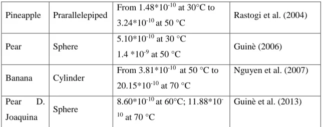
_a are usually estimated from experimental data. Examples of activation energy are reported in table 3:

Food Product Ea (kJ/mol) References

Carrot 28.36 Doymaz (2003)

Kiwi 20.41 Mhoammadi et al. (2008)

Tomatoe 33.32 Taheri-Garavant et al. (2011a) Pineapple Prarallelepiped From 1.48*10

-10 _{at 30°C to}

3.24*10-10 at 50 °C Rastogi et al. (2004)

Pear Sphere 5.10*10

-10 _{at 30 °C}

1.4 *10-9 at 50 °C Guinè (2006) Banana Cylinder From 3.81*10

-10 _{at 50 °C to} 20.15*10-10 at 70 °C Nguyen et al. (2007) Pear D. Joaquina Sphere 8.60*10-10 _{at 60°C; 11.88*10} -10 _{at 70 °C} Guinè et al. (2013)

Ginger slices 19.31 Akpinar et al. (2013)

Table 3 Activation energy of many fruit and vegetables.

A large number of empirical parametric equations expressing diffusivity as function of moisture content can be found in the literature. An empirical equation proposed by Kiranoudis et al., (1995) to calculate moisture diffusivity for all type of fruits and vegetables is as follow:

exp

exp

M

T

eff

b

c

D



a



_





_



_





_









(11) where:

M is the moisture content (kg/kgd.b.), T temperature in °C, a1.29 10 , 6 b 0.0725, c=2044.

A compilation of such equations is given by (Zogzas et al., 1996). All authors agree that the temperature effect can be described by an Arrhenius-type relation. Nevertheless, the moisture content effect has not yet been formatted into a general accepted model.

Hassini et al. (2007) for convective drying of potatoes, for moisture content from 2 to 0.25 kg/kgd.b. and for temperature ranging from 40 to 85°C, propose the following empirical equation for potato moisture diffusivity:





5 31580





T, M 7.18 10 exp exp 0.0025T 1.22 M T eff D R      _ _ _    _   (12)

that’s expressed in the form of:



T, M



exp exp



T



M T eff b D a _ _ _   c d _   (13)

The most common modelling in fruits involve heat and moisture transfer, equation 1 and 2, with empirical value of effective diffusivity such as that given by equation 11 and 13. Guinè et al. (2007a) proposed a model to describe the drying behaviour of pears. The model simulates a significant number of situations resultant from the variation of same of the operating conditions. The temperatures tested were 30, 40 and 50 °C, the air velocities were 0.5, 1.0 and 1.5 m/s, and the relative humidity of the drying air was 40%, 50% and 60%. The model was composed of two partial differential equations, accounting for the variations of temperature (T) and dry basis moisture content (M) for spherical geometries. Based on the model suggested by Zogzas et al. (1996), the effective diffusion coefficient (Deff) was expressed by Guinè as a modified Arrhenius relationship:





0





1 M T, M exp 1 T a eff E B D D CS R        _{   }    _{ } (14)

where Mand S represent the dry basis moisture and sugar concentrations, respectively. The parameters (D0, B, C,

E

a) were estimated from experimental data using an orthogonal

regression algorithm.

The model results, representing the evolution of moisture (H=M/1-M) with time for different radial positions, confirm the experimental observations that at the periphery the profile is far much steeper (corresponding to a very fast drying rate) than in the centre, where a smooth sigmoid curve was obtained (as a result of the paths for moisture diffusion being longer and more tortuous). This behaviour is totally opposite to that of sugar evolution, where a very fast increase in sugar concentration close to the border was found, making difficult the water diffusion.

1.2.3 Models considering shrinkage

Experimental data show that the final volume of air-dried food is reduced (Barcelos et al., 2011; Yadollahinia et al., 2009), therefore, predicting the shrinkage during dehydration becomes a prerequisite for process design and optimization of the drying conditions. In literature there are several empirical/theoretical models to predict the size reduction. This phenomena is the direct consequence of the combination of water elimination and a weak structure forming the solid network of the dried matrixes.

The shrinkage, SV, is generally defined as the ratio of the volume of the product during drying (V) over the initial volume (V0) or alternatively as reduced dimensional change of thickness, diameter or the ratio of surface to volume.

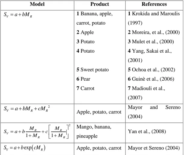
Different expressions are used to represent the shrinkage phenomenon. The mathematical relationships between these expressions are reported in table 4.

Model Product References V R S  a bM 1 Banana, apple, carrot, potato 2 Apple 3 Potato 4 Potato 5 Sweet potato 6 Pear 7 Carrot

1 Krokida and Maroulis (1997)

2 Moreira, et al., (2000) 3 Mulet et al., (2000) 4 Yang, Sakai et al., (2001) 5 Ochoa et al., (2002) 6 Guinè et al., (2006) 7 Madiouli et al., (2007) 2 V R R S  a bM cM

Apple, potato, carrot Mayor and Sereno (2004) 2 1 1 R R V R R M M S a b c M M     _{  }  _  _ Mango, banana,

pineapple Yan et al., (2008)





exp

V R

S  a b cM Apple, potato, carrot Mayor et Sereno (2004)

Table 4 Mathematical models to describe the shrinkage coefficient as a function of moisture

content in dried fruit and vegetables.

For some time shrinkage was considered negligible in drying modelling, thus making drying models easier to be solved. However, in food systems shrinkage is rarely negligible, in fact model considering shrinkage fit better experimental data than model without shrinkage. Mulet et al. (2000) showed that the volumetric shrinkage of potato samples follows a linear relation with moisture content at varying drying air temperatures, which suggests that the shrinkage is predominantly due to the volume of water removed. Such a linear shrinkage behavior of food materials has been reported by many researchers, whereas others reported a two-period phenomenon. In this case, the volume of water removed during the final stages of drying is larger than the reduction in sample volume. This behavior can be explained by the decrease in the mobility of the solid matrix of the material at low moisture contents. At lower drying temperatures, a more uniform moisture distribution exists, inducing less internal stresses that allow the sample to continue to shrink until the last stages of drying.

temperatures, case hardening of the surface may occur and the volume of the sample becomes fixed at an earlier stage, inducing less shrinkage and a more intensive pore formation.

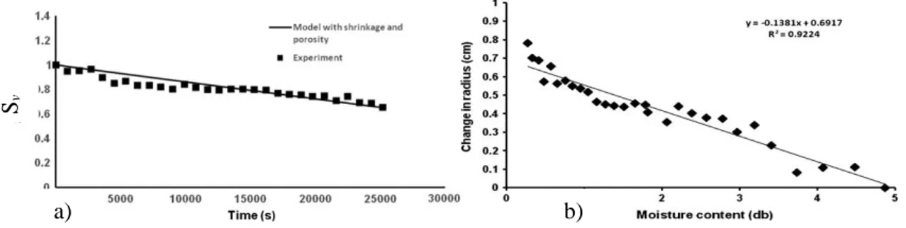
Parakeet et al. (2015) affirm that shrinkage and porosity change along with simultaneous heat and mass transfer during process. For potato slices dried for 7 hour at 62°C they observed that shrinkage vary linearly with moisture content and reduction in radial dimension of potato slices was around 35% (Figure 1). Porosity undergoes rapid increase after attaining certain moisture content in final stages of drying.

Fig. 1. a) Experimental measurements fitted with model considering shrinkage for potato,

b) Linear fitting of change in radius vs. moisture content, (Parakeet et al., 2005).

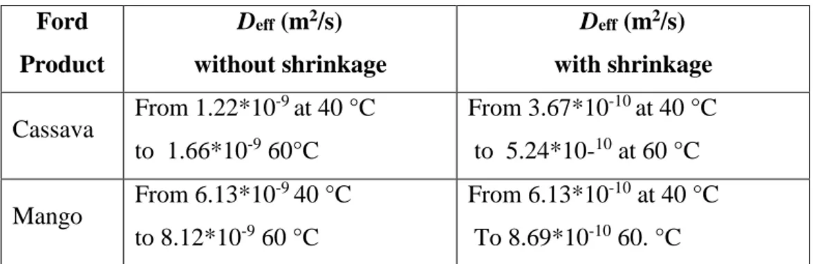
Hernandez et al. (2000), in order to obtain a simplified equation for the mathematical description of drying kinetics, proposed an analytical solution of a mass transfer equation with concentration-dependence shrinkage and a constant average water diffusivity. Experimental drying curves of 4 x 4 cm2 mango slices, with 0.5, 1.0 and 1.5 cm thicknesses and 10 cm long cassava parallelepipeds with 1, 2 and 3 cm thicknesses, at different air temperatures (50°C, 60°C and 70°C) and 3 m/s of air velocity were obtained in order to fit the proposed model by non-linear least-squares.

The values of effective diffusion coefficient obtained with and without shrinkage

are reported in table 5:

a) b)

Ford Product Deff (m2/s) without shrinkage Deff (m2/s) with shrinkage Cassava From 1.22*10 -9 _{at 40 °C} to 1.66*10-9 _60°C From 3.67*10-10 at 40 °C to 5.24*10-10 _{at 60 °C} Mango From 6.13*10 -9 _{40 °C} to 8.12*10-9 60 °C From 6.13*10-10 at 40 °C To 8.69*10-10 60. °C

Table 5 Daff for cassava and mango with and without shrinkage, (Hernandez et al., 2000).

They obtained an accurate simulation of experimental data using the average water diffusivity and shrinkage parameter.

Hasina et al. (2007) plotted the variation of the experimental volume of potato samples as a function of the mean moisture content (Fig. 2).

Fig. 2. Volume of potato slab vs moisture content for different air temperatures,

(Hasina et al., 2007).

They fitted the experimental data by a linear equation:

0 0 0 V V M V V V F VF



  (15)

where V_F is the final (dry) product volume, V is the initial product volume. The shrinkage ₀ coefficient is calculated as the slope of the best fit.

In their experiments





1.37

is calculated on the entire temperature domain: 45-85 °C. It can be compared to 1.35 (Chekhov et al., 2004) for potato, 1.54 for grapes (Venegas, et al.,

0 0.2 0.4 0.6 0.8 1 1.2 0 1 2 3 4 5 M (kg/kgd.b.) T a = 40 °_C T a = 55 °_C T a = 70 °_C °_C T a = 85

The differences between the moisture diffusivity data, corrected and non-corrected for shrinkage, are very significant in the domain of critical value of M, nearly one order of magnitude. Tari (°C) air (m/s) Deff (m2/s), without shrinkage Deff (m2/s), with shrinkage Relative difference (%) 40 0.5 4.01 · 10-9 _{4.24 · 10}-10 _89.27 1 4.12 · 10-9 4.30 · 10-10 89.70 55 0.5 4.39 · 10-9 8.12 · 10-10 81.50 1 4.45 · 10-9 8.34 · 10-10 81.25 70 0.5 5.36 · 10-9 1.20 · 10-9 77.61 1 5.43 · 10-9 1.29 · 10-9 76.24 85 0.5 6.13 · 10-9 1.88 · 10-9 69.33 1 6.22 · 10-9 1.92 · 10-9 69.13

Table 6 Analytically determined moisture diffusivity, with and without shrinkage at different

temperatures and air velocities, (Hassini et al., 2007).

Barcelos et al. (2011) modelled the drying kinetics of potatoes considering shrinkage, adding a low of variation of the radius of the potatoes (a sphere shape with initial radius of 10 mm), obtained fitting the experimental data (equation 16).

1 3 0 0 0.8 M r r 0.8 M      _    (16)

During drying, the operating conditions of the oven were: an air temperature of 60ºC and absolute humidity of 5 kg/100 kgdry air.

They solved the differential equation of mass transfer for moisture content inside the spherical potatoes using the method of finite control volume.

Figure 3 depicts the experimental and simulated data of dimensionless free moisture content as a function of the drying time. In the beginning of drying, the diffusive model, not taking into account the shrinkage, fits better the data. After, this model underestimates the internal mass transfer phenomena as it does not take into account the changes in internal resistance promoted by the size reduction over time, leading to a significant effect on describing the

Fig. 3. Dimensionless free moisture content as a function of drying time, (Barcelos et al., 2011).

In figure 4 they plotted the moisture content profile along with radius axis. At the beginning of drying (i. e. 3600 s) the moisture content inside the food remains almost spatially uniform and the moisture content shape profile is a sigmoid. From time 10800 s to 36000 s the moisture content shape profiles are parabolic.

Fig. 4. Dimensionless free moisture content as a function of dimensionless radius axis at a given

drying time, (Barcelos et al., 2011).

Brasiello et al. (2013) proposed two mathematical models with shrinkage effect describing eggplant drying. In the first model they considered shrinkage effect through a non-constant diffusion coefficient depending on the water content, D_eff   M_R, where



is the intercept of D_eff

 

M_R and  the slope of D_eff

 

M_R .While in the second model they introduced a fictious convective term, _u MR

x   

 , where u is the shrinkage velocity and



a parameter linking

u

and the spatial derivate of M . They demonstrated, using _R

[(M -M e )/ (M 0 -M e )] [(M -M e )/ (M 0 -M e )] Dimensionless radius [r/r0]

data of weight loss and void fraction at different temperature they derived models parameters. The advantage of this model was of describing with sufficient accuracy the drying process in a wide range of conditions using few parameters.

Fig. 5. Experimental and predicted total dimensionless water content temporal profiles during

eggplant drying at different temperatures, (Brasiello et al., 2013).

In a successive work, Brasiello et al. (2017) analyzed the possibility of prediction MRI spatial profile of water during eggplant’s dehydration using the mathematical model developed previously. In figure 6 it’s compared the MRI derived moisture spatial profile during the dehydration of a cylindrical sample of eggplant at 323 K with the previous model taking into account the shrinkage effect. It’s possible to see that numerical data are close to experimental data, instead applying simple Fick’s law in cylindrical coordinate, numerical data are lower than experimental data.

1.3 Techniques for quality analysis of fruit and vegetable

Laboratory analysis of food quality often involves extensive preparation procedures, during which foods are severely disturbed by size-reducing, deforming, or diluting steps. This is very unlike the way in which food consumers evaluate the quality of food products (i.e., foods are consumed while their integrity is generally intact.). Naturally it would be desirable to be able to analyse food quality in a completely non-destructive and non-invasive way. Nuclear magnetic resonance (NMR) techniques are among those most capable of performing such a task.

Nuclear magnetic resonance (NMR) spectroscopy and magnetic resonance imaging (MRI) are based on the magnetic properties of the atomic nucleus and many elements have isotopes with such properties, above all the omni-abundant proton. NMR and MRI have some distinct advantages over other instrumental methods: they are non-invasive and non-destructive; most systems are transparent for the excitation; they measure volumes instead of surfaces; and the methods allow the extraction of both physical and chemical information. By exploitation of magnetic resonance it is possible to obtain unique knowledge about, for example, flow, diffusion and water distribution without perturbing the system. Similarly, processes such as heating, freezing, salting, hydration and dehydration can be monitored absolutely non-invasively.

Another advantage of these techniques, beside that the sample don’t need any pre-treatment, is that once developed, standards protocols based on rapid measurements can be easily transferred to quality control applications.

1.3.1 Basic theory of NMR and MRI

NMR differs from most other forms of spectroscopy in that it is the atomic nuclei that are the subject of study, and the energy absorbed and emitted by the nuclei is in the radio frequency range. Many nuclei possess an angular momentum, which means that they have a characteristic spin quantum number (I), and may be analyzed using NMR. The most common nuclei analyzed by NMR are the proton (H) and the 13_{C isotope of carbon, as well as} 19_{F and} 31_{P, all of which have a spin I = 1/2.}

These nuclei are also charged, and a spinning charge generates a magnetic field. Simply put, the nuclei behave like tiny magnets that interact with an applied, external magnetic field. Once the nuclei are placed within a strong external magnetic field (B0), the spin of the nuclei will align with that field. Because of quantum mechanical constraints (nuclei of spin I have

that the spin 1/2 nuclei can adopt: either aligned with the applied magnetic field (parallel or spin +1/2) or aligned against the field (anti-parallel or spin −1/2). The parallel orientation has a slightly lower energy associated with it and, therefore, has a slightly higher population. It is this excess of nuclei in the spin +1/2 state that produces the net magnetization that is manipulated during an NMR experiment. The spin of the nuclei is not around the center axis, but comparable to a gyration.

The motion of a spinning charged particle in an external magnetic field is known as precession, and there is specific precessional orbit and frequency, the Larmor frequency, which is related to the magnetic properties of the nuclei. The magnitude and direction of the local magnetic field describe the magnetic moment or magnetic dipole of the system. However, due to the precession and the lower energy state excess of nuclei, there is a net vector parallel to the applied field.

All nuclei of the same element, H for example, will have a nearly identical Larmor frequency in a magnetic field. The specific frequency is dependent on the strength of the external magnetic field, and the Larmor frequency of H in this field defines the NMR instrument. For example, a proton has a Larmor frequency of 500MHz in an 11.7 T magnet, so the instrument is termed a “500MHz NMR spectrometer.” The strength of the magnet not only governs the Larmor frequency of the nuclei, but also determines the degree of excess nuclei in the parallel orientation. The excess of nuclei in the parallel orientation increases with an increase in the external magnetic field strength, and this in turn impacts the signal intensity of the NMR experiment (i.e., more protons will be detected in a higher field strength instrument). This is one reason researchers seek ever more powerful magnets for NMR. Field strength impacts sensitivity and the signal/noise (signal-to-noise) ratio, and, therefore, the information obtained from the NMR experiment.

One of the major developments in NMR technology was the RF pulse, in which a large range of frequencies is excited by a short pulse of RF energy around a centered carrier frequency, which is at the Larmor, or resonance, frequency of the nuclei under study. This pulse simultaneously excites all of the protons in the sample. The NMR data for all the protons is collected during a short time after the pulse is applied; therefore, it is termed time-domain NMR. In NMR, the carrier frequency, transmitter power, and duration of the RF pulse determine the frequency range of the pulse.

However, after a pulse of RF energy is applied to the system, the nuclei precess coherently and individual nuclei absorb energy and shift to a higher energy state. The pulse, which is applied by a transmitter coil perpendicular to the z-axis (B1), tilts the net magnetization vector away from the z-axis and toward the xy plane .

Although the parameters that define a pulse include the transmitter power and the pulse duration, a specific pulse used in an NMR experiment is usually described by the degree to which the net magnetization is tilted. The most common pulse is the 90◦ pulse, which tilts the net magnetization exactly into the xy plane where the receiver coil is located, thereby maximizing the resulting signals.

Many NMR experiments use a series of pulses, termed a pulse sequence, to manipulate the magnetization. Complex pulse sequences are essential for the two-dimensional (2D) NMR experiments that are required for complete structural analyses of complex molecules. Once the net magnetization has been tilted into the xy plane by a 90◦ pulse, the magnetization begins to decay back to the z-axis. This process is termed NMR relaxation, and it involves both spin–lattice (T1) and spin–spin (T2) relaxation. T1 relaxation is associated with the interaction of the magnetic fields of the excited-state nuclei with the magnetic fields of other nuclei within the “lattice” of the total sample.

T2 relaxation involves the interactions of neighboring nuclei that lead to a diminishment in the energy state of the excited-state nuclei and the loss of phase coherence.

The mechanisms behind relaxation are complex, but the process can be utilized for some specific NMR experiments that, among other things, take advantage of the fact that samples in different forms, liquids vs. solids for example, relax at different rates.

Like NMR spectroscopy, MRI is a method that exploits the magnetic properties of the atomic nucleus. Magnetic resonance imaging (MRI) is unique in that the sample can be placed into the magnet in the native form, and 2D or 3D images of the sample can be generated.

MRI involves variations in field strength and the center frequency of the pulses over time and space, along with the application of field gradients in different geometric positions relative to the magnet bore (B0). The end result is a spatial “encoding” of the sample protons with different phase and frequency values. After multidimensional Fourier transformations of multiple FIDs from different spatial “slices” of the sample, an image of the sample is produced that contains information about the state of the material under study.

1.3.2 NMR applied to fruit and vegetables

Low-field 1_{NNMR relaxometry is an appreciate technique to investigate on the most} abundant components of intact foodstuff based on relaxation parameters and amplitude of the NMR signals. 1H pulsed low field NMR allows to obtain information on water compartmentalization and diffusion by detecting proton signal predominantly due to H2O contained in vegetable tissue.

In literature many fruits such as banana (Raffo et al., 2005), tomato (Musse et al., 2010), kiwifruit (Panarese et. al., 2012) have been investigated by means of low field NMR. The relaxation signals from vegetal cells have generally been described by a multi-exponential behaviour reflecting different water compartments. The longitudinal T1 and transverse relaxation T2 times are known to be related to the water status in the compartments, i.e. water content, water mobility and interactions between water and macromolecules.

Few investigations have been focused on the attribution of the NMR signal components to water compartments.

In tomato fruit Tu et al. (2007) reported a single component of T2, while four components were found in the tomato pericarp by Duval et al. (2005) and Maringheto et al. (2009). The precise assignment of the NMR signal components to specific subcellular compartments is still a subject of database.

Maringheto et al. (2008) investigated the internal sub-cellular characteristics of Red Delicious apple with novel two-dimensional NMR relaxation and diffusion technique. They found four relaxation peaks. The peak with the longest T2 and largest area was associated with water in the vacuole, the peak with shortest T2 was associated to rigid components of cell wall in the apple matrix, and the other two were associate with the water in the cytoplasm and extra-cellular compartments.

Fig. 7. Distribution of transverse water proton relaxation times in fresh ‘Red Delicious’ apple

tissue measured at spectrometer frequency of 23.4MHz with a CPMG 90–180◦ pulse spacing of 200s. Numbers refers to relaxation peaks of the water proton in the different cell compartments: 1, the vacuole; 2 and 3, cytoplasm and extra-cellular compartment and 4,

cell wall,(Maringheto et al., 2008).

There are also available portable NMR devices that allow easy sample access, which makes them attractive for quality control in industrial environments and directly on sealed packaged food. In this case, the magnet is placed to one side of the object fully preserving the integrity and the dimension of the sample under investigation and also allowing the measurement to whole packed products.

Fig. 8. Sketch of the geometry of the magnet of the profile NMR mouse.

Capitani et al. (2010, 2013) monitored the water status of kiwifruits as a function of season using a single-sided NMR sensor. Using this sensor, they measured the entire fruit at a depth of about 0.5 cm from the peel surface without cutting it, as shown in figure 9.

Fig. 9. Measurement of intact kiwifruit with a single-sided NMR sensor,

(Capitani et al., 2010).

The T2eff distribution of a mature kiwifruit showed three peaks, as reported in figure 10. According to the literature, they assigned the longest T2eff component to protons in vacuole, the intermediate one to proton in cytoplasm and extra-cellular space, and the shortest one to proton in cell walls.

Fig. 10. Transverse relaxation times distribution measured on ripened kiwifruit,

(Capitani et al., 2010).

In a successive work Capitani et al. (2013), monitored the ripening of kiwifruits in field on fruit attached to the plant during three campaigns of measurement carried out in October, November and December (figure 11).

Fig. 11. Measurement in field on entire kiwifruit attached to the tree with a portable unilateral

NMR instrument, (Capitani et al., 2013).

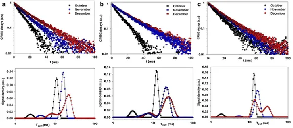
Figure 12 show the transverse relaxation decays measured in field on entire kiwifruit attached to the tree, for three cultivars.

Fig. 12. Transverse relaxation curves measured in field in October, November, and December on

Hayward (a), CI.GI (b), and Zespri (c) with the corresponding relaxation time distribution, (Capitani et al., 2013).

In all cultivars, a lengthening of decay with the season was observed; already the process was complete in November for Zespri as shown by the perfect overlapping of decay measured in November and December.

Capitani et al. (2014) also applied NMR methodology to the analysis of blueberries.

Fig. 13. (A, B and C) Depth profiles of three fresh blueberries, and profile of the same blueberries

let to wither for three and six days, (Capitani et al., 2014).

They compared profiles of three fresh intact blueberries to those let to wither outside the fridge for three and six days. The amplitude profile of withered blueberries was found to be lower than measured on fresh blueberries, indicating a loss of water.

They calculated the average loss of water in withered blueberries by integrating the profiles. After three days they measured a loss of water of 13 %, 11 % and 16 % in three different blueberries.

Instead, from transverse relaxation time measurement, obtained for the three fresh blueberries and the same let to whiter for three and six days, they found a bimodal and trimodal distribution for fresh and withered blueberries, respectively.

Fig. 14. T2 distributions of three fresh blueberries, and the same blueberries let to wither for three

days, and for six days, (Capitani et al., 2014).

In fresh blueberries, the longest component of T2 was assigned to protons in vacuole and cytoplasm, the shortest in cellular wall.

After three and six days of withering, the shortest T2 values was assigned to protons in cellular wall, the intermediate in cytoplasm and the longest in protons to vacuole. After withering for six days T2 value shortened, indicating membranes denaturation and occurrence of water loss due to prolong whitening. This observation may be explained with a reduced permeability of water across membranes.

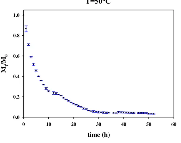
Adiletta et al. (2015) used the NMR relaxometry to investigate the drying process of parallelepiped samples of pear at T=50°C. Using a portable NMR they measured the amplitude of water profile in fresh and dried samples during time, which resulted in good agreement with gravimetric measurements. Moreover, information on shrinkage was obtained by measuring the depth of NMR profiles during time. The data obtained were well correlated (R2=0.87) with size measurements made through a vernier caliper.

Adiletta et al. (2014) investigated the effect of hot-air drying (50, 60 °C) on the physical properties of cylindrical eggplant samples. They determined drying kinetics, water profiles along longitudinal and transversal sample sections through nuclear magnetic resonance imaging (MRI) and volumetric shrinkage.

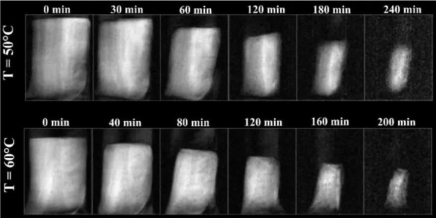
The two-dimensional spin echo images of eggplant samples are shown in figure 15 for both temperatures they investigated (50, 60 °C) at specific times.

Fig. 15. Two-dimensional spin echo images of eggplant at both investigated temperatures and

selected drying times, Adiletta et al. (2013).

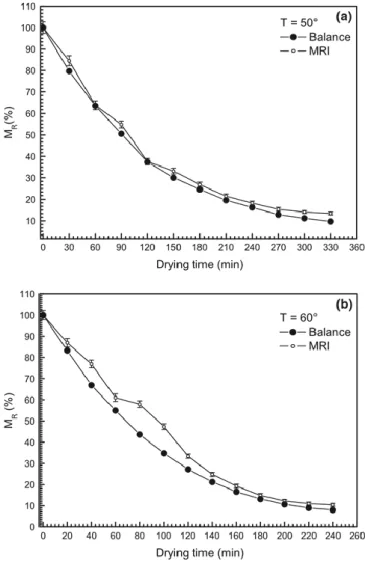
As expected, during the drying process, the size of brighter regions, which corresponded to higher proton density areas, considerably decreased. For every temperature, they extracted the pixels with the maximum and minimum signal, regardless the drying steps, considering all the images collected. Then they rescaled all the values: the minimum pixel value was set equal to 0 and the maximum value to 1. After that, for each image, they summed all the pixel values and normalized all data to the initial mass of water, to obtain the dimensionless moisture ratio MR. At the end they compared these values with those obtained with gravimetric method achieving a good agreement, figure 16.

Also, they proposed a power equations (

V V

₀

 

a

₁

a M

_{2 R}b) to fit the experimental data of shrinkage, figure 17.

Fig. 16 Moisture ratio (%) of samples during drying obtained by gravimetric method and MRI at

T = 50 °C (a) and 60 °C (b), (Adiletta et al., 2014).

Fig. 17. Experimental shrinkage data and prediction by power model, (Adiletta et al., 2014). M/M0