Table of contents
Introduction 3
Chapter 1 9
Chapter 2 49
Chapter 3 89
Conclusions 130
Introduction
This PhD thesis is composed of three chapters having the aim to contribute to the literature about corporate bankruptcy and firm’s exit. The choice to investigate this phenomenon is due to the importance of this subject since corporate failure leads to relevant costs for the whole economy, and, especially after the financial crisis, it tended to involve several aspects and actors of business life. The relevant number of bankruptcies, together with the growing incidence of major companies collapse, in the last years, led to a rise in the number of insolvency related job losses. Indeed, failures can be characterized by insolvencies which undermine the creditors of defaulting companies and create chain of bankruptcies. Furthermore, the default is likely to affect company’s shareholders since the opening of a collective procedure leads to direct costs management systems: compensation for dismissal, lawyers' fees, costs of procedures, etc. These costs weigh on the business value and particularly on insiders. Indeed, at first glance, it is quite obvious that business failures cause losses for the agents directly concerned, in particular employees, creditors and owners of companies which tends to suggest an overall negative assessment of failures from the point of view of the community. But bankruptcy can also generate indirect costs consisting in losses for the company partners, increase of unemployment and decrease of incomes in a given area, or supplier credits and difficulties in obtaining financing. The indirect costs can be high and should not be ignored in the analysis of the consequences of corporate bankruptcy. This is all the more justified that, according to the concept of Corporate Social Responsibility, the objectives of a business go far beyond the insiders’ interest. Firm should thus achieve a sustainable development in the broad sense of economic development that, in addition to creating value for shareholders, maintains a conservation of the natural and social environment and human capital. As the impact of corporate failures concern a large number of agents, an important attention must be paid to this important and expanding phenomenon.
The declining trend in business insolvencies initiated in 2010, has continued in 2016 for the seventh consecutive year. Companies have absorbed the 2008 crisis shock at the global level but they remain vulnerable to the lack of solid macroeconomic and financial environment and to local hot spots. In 2016 they faced three major global headwinds: (i) the sluggish global economy, with real GDP growth posting only +2.5% in 2016 (versus +2.7% in 2015); (ii) the sharp slowdown in global trade, with export volume growth reaching an unprecedented blow at +1.9% (+3.1% in 2015); (iii) fierce price competition, which has put
turnovers under pressure; and (iv) volatility in exchange rates and international financial flows, which have kept financing under constraints (Euler Hermes, 2017). Western Europe is the only region to record a sizable decline in bankruptcies in 2016 (-5% after -13% in 2015), thanks to the gradual improvement of the economic situation. Despite these positive results, the level of bankruptcies in Western Europe remains high. As Figure 1 shows many countries still report more insolvencies in 2016 than their 2003-2007 average. In 2016, for instance, Spain and Portugal recorded 341% and 82 % more bankruptcies than before the crisis. The picture is already less troubling for Italy (+38%) and France (+27%), where the decline is supported by the recovery of corporate margins and strong fiscal boosters.
Figure 1: 2016 Insolvencies compared to 2003-2007 average (% change)
Source: National Statistics, Euler Hermes
Keeping firms alive is a public policy target since bankruptcy has not only financial consequences but industrial ones too, linked to the loss of precious intangible assets and
know-how that represents a source for the whole economy. It represents, thus, a phenomenon which has a negative influence on the competitiveness of the business environment.
Exit is a common consequence of firm’s poor performance. Firms that underperform as they compete in the market will, sooner or later, exit the market. It is a process of selection results from a (passive) process of post-entry Bayesian learning: those firms which discover to be efficient enough to ensure non-negative profitability, rationally choose to continue their operations and grow, while the others quit the market (Jovanovic, 1982). This process is better worth knowing for a main reason: the Shumpeterian concept of creative destruction, which describes the process of transformation that is linked to radical innovation, which supposes the replacement of established companies by new entrants, involves the exit of a certain number of existing firms. Besides this renewal of productive system it ensures, exit can also have a positive value since individuals who have closed down the company they owned or managed in the previous year are more likely to engage successfully in a future entrepreneurial activity (Levratto, 2013).
Different studies have, thus, attempted to identify the causes of corporate bankruptcy. A comprehensive vision of the possible causes of failure is provided by Bradley and Rubach (2002) who remind the different families of the factors identified as causes of insolvency. Management, marketing, or financial reasons are the main ones, but additional elements may intervene, such as outside and inside business condition, tax issues or disputes with a particular creditor. Starting with the seminal work of Altman (1968), a large body of literature has investigated corporate bankruptcy with a focus on firm-specific features, searching to predict insolvency through the application of several statistical methods on economic and accounting data. In his seminal study on bankruptcy detection, Altman improved research methodology by usage of multiple discriminate analysis (MDA) where the discrimination was determined by a score–the «Z-score»–calculated on the basis of five accounting ratios. Recently, some authors have resorted to artificially intelligence expert system (AIES) models for bankruptcy prediction. These recent artificially intelligence expert system models would lightly outperform discriminant and logistic analysis but they are based on complex underlying model structures. Hence, standard implementations have to be modified to allow the estimation of realistic default propensities. A correct measure of firms’ insolvency risk is very important both for internal monitoring purpose and for the potential investors, stockholders, actual or potential firm’s competitors.
The first chapter of this PhD thesis goes in the direction of this strand of literature, with the purpose to provide an instrument able to predict corporate bankruptcy. The study is
entitled “Predicting corporate bankruptcy by a composite indebtedness index. An application to Italian manufacturing firms”, and proposes a Composite Indebtedness index of financial ratios, estimated by a Robust Principal Component Analysis for skewed data, that allows to classify firms according to two dimensions: their indebtedness degree and their solvency capability. Furthermore, the study presents a logit model aimed at investigating if and to what extent the proposed index is able to correctly predict firms’ financial bankruptcy probabilities. The econometric results are compared with those of the popular Altman Z-score for different lengths of the reference period. The empirical evidence suggests a good performance of the proposed Composite Indebtedness index which, therefore, could be used as an early warning signal of bankruptcy. This study contributes to the literature in several ways. First, since small sample size appears to be a limitation, it considers the Italian manufacturing companies as a whole and includes small, medium and large firms in a large industry sample. Secondly, I attempt to improve the research model by implementing a composite analysis based on both Principal Component Analysis (PCA) and logit model, demonstrating that the combined method of PCA and logit estimation is promising in evaluating firms’ financial conditions. Thirdly, I attempt to evaluate the efficiency of the model, that is its economic and organizational usability in an operational context.
Generally, the focus of the accounting and finance literature has typically considered only the internal features of a company (financial and non-financial information) to determine its likelihood of failure. Only very recently, a small number of studies analysed the influence of institutional features of the local context to understand the exit behaviour across geographical regions. This is a relevant issue to address since the likelihood of firm’s exit is likely to be determined by how much favourable are market conditions to sustaining businesses primarily dependent on local demand.
The second chapter of this PhD thesis entitled “New firms’ bankruptcy: does local banking market matter?” tries to fill this gap. It analyses the role that local context and particularly the role that local banking market, may exert in shaping new firm’s bankruptcy. The novelty of this study results from three main elements: the emphasis put on the relationship between insolvency and the organization of the local credit market, the estimation technique used (Logit Multilevel Model) and the sample of companies considered in the empirical analysis based on Italian new firms (incorporated between 2008 and 2013). According to many research studies on bankruptcy, new firms are more likely to exit from the market than other firms (Thornhill and Amit, 2003) and are very vulnerable to the
macroeconomic environment (Bonaccorsi di Patti and Gobbi 2001). New and young companies are the primary source of job creation in economies, contributing to economic dynamism by injecting into the market competition and innovation. At the same time, these firms are the most financially vulnerable in the market. This weakness leads to questioning the role played by the financial system and, more precisely, by banks, in the local economic activity and as a driver of the performance of local firms. The results suggest that a higher level of financial development in a province decreases the likelihood of a new firm’s bankruptcy. In addition, the estimations suggest that the effect of local financial development and bank concentration is shaped by size. The effect that local financial development exerts in reducing corporate bankruptcy is stronger for small start-ups, which traditionally suffer from great difficulty in accessing credit, whereas local banking concentration reduces the probability of bankruptcy for large, new firms.
The third chapter of this PhD thesis entitled “Spatial patterns and determinants of firm’s exit in France” is also in line with the strand of literature which investigates the effect that location specific determinants may have in shaping the exit risk in the local area. The purpose of the study is to understand the relevance of the domino effect in firm’s exit among neighbour locations with a focus on two regional variables: local specialisation and local financial development. Indeed, the influence of location can be considered also looking at the effect of agglomeration economies and spatial dependences. The observation that economic activity tends to be clustered in space (Porter, 1998; Cooke, 2002), suggests that agglomeration economies are relevant and can compensate for the negative effect of density such as intense competition from other firms located in the vicinity which may lead to relatively intense competition on the input-side as well as on the output-side of the market. The analysis refers to the Exit Rate of French Departments (corresponding to NUTS3 in the EU classification) over the period 2009-2013. I propose an econometric study based on a dataset combining different sources computed at the Department level based, and on the application of spatial econometric techniques to consider the spatial dependence in business failure. The results suggest that firm’s exit is characterized by positive spatial autocorrelation, so that locations with high exit rates tend to be surrounded by similar ones. In addition, similarly to the second chapter, I find that a higher local financial development reduces the exit rate of a department whereas local specialisation seems not to exert any effect. Therefore, by highlighting the clustering phenomena, I contribute to the spatial literature that emphasizes the neighbouring effect and states the idea that what happens in a certain area not
only depends on the local context but also on what happens in the nearby areas. Some policy implications conclude each chapter of the thesis.
References
Altman E. (1968) Financial ratios, discriminant analysis and the prediction of corporate bankruptcy. Journal of Finance 23(4) :589–609.
Bonaccorsi di Patti E, Gobbi G (2001) The changing structure of local credit markets: Are small businesses special?. Journal of Banking and Finance 25(12): 2209–2237 Bradley, DB, & Rubach, MJ. (2002) Trade credit and small business: A cause of business
failures. Technical report: SmallBusiness Advancement National Center, University of Central Arkansas.
Cooke P (2002) Knowledge economies. Clusters, learning and cooperative advantage. Routledge Studies in International Business and the World Economy (26), xii, 218 .Euler Hermes (2017), Insolvencies: the tip of the iceberg. Special focus on state owned enterprises around the world. Economic Outlook no. 1230-1231 available at
http://www.eulerhermes.no/no/economic-research/economic- publications/Documents/Economic-outlook-insolvencies-the-tip-of-the-iceberg-jan-17.pdf
Jovanovic B (1982): Selection and the Evolution of Industry, Econometrica, 50: 649– 70.Levratto N (2013), From failure to corporate bankruptcy: a review Journal of Innovation and Entrepreneurship
Porter M E (1998) Clusters and the new economics of competition. Harvard Business Review, 76(6):77–90
Thornhill S, Amit R (2003) Comprendre l'échec: mortalité organisationnelle et approche fondée sur les ressources. Document de recherche. Direction des études analytiques, Statistique Canada 11F0019-202.
CHAPTER 1
Predicting Corporate Bankruptcy by a Composite Indebtedness Index. An
Application to Italian Manufacturing Firms.
Abstract
Starting from a series of financial ratios analysis, I build up two indices which take into account both the firm’s debt level and its sustainability. The construction of a Composite Indebtedness index, based on an original use of Robust Principal Component Analysis for skewed data, allows to classify firms according to their indebtedness degree and nature. This is a first tool to evaluate firms’ financial health. Secondly, a model aimed at investigating if and to what extent the proposed indices are able to correctly predict firms’ financial bankruptcy probabilities is proposed. The econometric results are compared with those of the popular Altman Z-score for different lengths of the reference period. The empirical evidence would suggest a good performance of the proposed Composite Indebtedness index which, therefore, could also be used as an early warning signal of bankruptcy.
Keywords: Financial Ratios, Bankruptcy, Robust PCA, Z-score, Logit.
1. Introduction
Due to the international financial crisis, both the number and the average size of bankrupt firms has increased dramatically with the consequent greater interest from governments, financial institutions and regulatory agencies.
A correct measure of firms’ insolvency risk is very important both for internal monitoring purpose and for the potential investors, stockholders, actual or potential firm’s competitors. The purpose of this study is to construct, analyse and test a new bankruptcy prediction model which can be easily applied as early warning instrument. The potential application of this model is in the spirit of predicting bankruptcy and aiding companies’ evaluation with respect to going-concern considerations, among others, since the early detection of financial distress facilitates the use of rehabilitation measures. Insolvency is mostly a consequence of a sharp decline in sales which can be caused by several and different factors like a recession, deficiencies of management, relevant changes in market dynamics, shortage of a row material, changes in lending conditions, etc. An early warning signal of probable bankruptcy is very important since it will allow to adopt preventive and corrective measures. This study aims to contribute to the elaboration of efficient and effective corporate failure prediction instruments in order to prevent bankruptcy through the adoption of reorganization strategies. Failure, indeed, is not identifiable in a specific episode but in a process of progressive worsening of the financial health of a company. Given the dynamic nature of firms’ financial crisis, it is necessary to build an early warning index for firms’ insolvency which could signal a critical level of over-indebtedness behind which the financial status of the firm becomes pathological, therefore very difficult to rehabilitate.
Most of the past studies concentrate on specific industrial sectors and/or used a relatively small sample of firms. These studies include models for manufacturers by Beaver (1968), Altman (1968), Wilcox (1971, 1976), Deakin (1972, 1977) and Edmister (1972), among others, and models for specific industries such as Altman on railroads (1973), Sinkey on commercial banks (1975), Korobow and Stuhr (1975) and Korobow et al. (1976) on commercial banks, Altman and Lorris on broker/dealers (1976) and Altman (1977) on savings and loan associations.
Beaver (1966), Altman (1968) and Van Frederikslust (1978) argue that, although a failure may be caused by several circumstances, the development of some financial ratios can be a signal of the firm’s financial health. Previous studies indicate that, with few financial ratios, corporate bankruptcy can be predicted with success for at least five years before failure. Important shortcomings, however, characterize previous works. First, financial ratios are
chosen if they perform well, so without a specific reference to financial theory. Moreover, a very small sample of firms are considered in the empirical analysis. Therefore, the results obtained in these works cannot be generalized.
This study contributes to the literature in several ways. First, since small sample size appears to be a limitation and “… any new model should be as relevant as possible to the population to which it will eventually be applied” (Altman et al., 1977, p.30), it considers the Italian manufacturing companies as a whole and includes small, medium and large firms in a large industry sample. Secondly, I attempt to improve the research model by implementing a composite analysis based on both Principal Component Analysis (PCA) and logit model. I demonstrate that the combined method of PCA and logit estimation is promising in evaluating firms’ financial conditions. Thirdly, apart from effectiveness, I also attempt to evaluate the efficiency of the model, that is its economic and organizational usability in an operational context (Cestari et al., 2013). With reference to the actual usability of the model on the part of the potential users, this model proposes two steps/instruments in the analysis: 1) an accurate, but rather simple, bankruptcy prediction instrument which allows to classify firms in different categories with respect to their solvency status on the base of financial ratios; 2) a more complex logit model, based on both the first step computed indices and additional non-financial variables, which allows to compute specific bankruptcy scores (predicted probabilities) for each firm included in the analysis. Finally, the logistic regression estimates are compared with those of the popular Altman Z-score for different lengths of the reference period. Hence, in addition to several models that have been tested by the relatively short one-year prediction horizon, the predictive power of the index several years prior to bankruptcy is tested.
In brief, I extend previous methodology by building a very large sample of firms and paying attention to both financial and non-financial firms’ characteristics. Moreover, I examine how the model can be used in practice to analyze the risk of failure. In this context, I first derive a simple decision rule to classify firms as either at high risk of failure or at low risk of failure. I then propose a more complete model to predict the risk of failure as early warning signal of bankruptcy. The chapter is organized as follows. Section 2 summarizes the related literature, Section 3 illustrates the methodology, Section 4 shows an application to Italian manufacturing firms and illustrates the empirical findings. Section 5 concludes.
2. Literature review
Bankruptcy has been the subject of numerous studies over the past years2. Researchers have investigated both the causes and the legislative and financial tools available to start a process of recovery/rehabilitation of the firm. Especially after the recent international financial crisis, there has been a general need to predict insolvency and financial failure on-time in order to take corrective and remedial measures for protecting business from the problem of bankruptcy.
A broad international field of study has focused on predicting bankruptcy using statistics and economic-financial indicators. Prior to the development of quantitative measures of company performance, agencies were established to supply qualitative information assessing the creditworthiness of firms. During the 1930s many models were developed to help banks decide whether or not to approve credit requests (Smith, 1930; FitzPatrick, 1932; Ramser and Foster, 1931; Smith and Winakor, 1935; Wall, 1936). Bellovary et al. (2007) traced a brief historical summary of the early studies (1930 to 1965) concerning ratio analysis for bankruptcy prediction that laid the groundwork for the studies that followed.
At the end of the 1960s, several applications of univariate and multivariate statistical methods were developed. One of the classic works in the area of ratio analysis and bankruptcy classification was performed by Beaver (1968). His univariate analysis of a number of bankruptcy predictors set the stage for the multivariate attempts. Beaver found that a number of indicators could discriminate between matched samples of failed and non-failed firms for as long as five years prior to failure, but he completed a discriminant analysis on a single ratio (cash flow/total debt).
Altman (1968) and Deakin (1972) applied multivariate analysis, followed by several authors (Blum, 1974; Elam, 1975; Libby, 1975; Alberici, 1975; Taffler, 1976, 1982; Altman et. al., 1977, 1993; Wilcox, 1976; Argenti, 1976; Appetiti, 1984; Forestieri, 1986; Lawrence and Bear, 1986; Aziz, Emanuel and Lawson, 1988; Baldwin and Glezen, 1992; Flagg, Giroux and Wiggins, 1991; Bijnen and Wijn, 1994; Kern and Rudolph, 2001; Shumway, 2001; Hillegeist, et. al., 2004; Altman, Rijken, et. al., 2010). In his seminal study on bankruptcy detection, Altman (1968) improved research methodology by usage of multiple discriminate analysis (MDA) where the discrimination was determined by a score–the «Z-score»– calculated on the basis of five accounting ratios. Thus, only five financial ratios were enough
2 For comprehensive reviews on predicting corporate bankruptcy methodologies, see Aziz and Dar (2006),
to distinguish healthy from unhealthy companies. The first research on SMEs failure was done by Edminister (1972) who also used MDA as statistical technique to discriminate among loss and non-loss SME borrowers. The empirical analysis, based on a MDA model with seven financial ratios, revealed that the models with industry relativized ratios were characterized by higher classification accuracy in comparison with models based on classical ratios.
After Altman’s seminal study, the linear discriminant analysis has been intensively used in practice mainly because of the simplicity of its application. However, Johnson (1970) and Joy and Tollefson (1975) have criticized the excessive broadness of the so-called grey area and the difficulty of application in predicting bankruptcy ex ante. Guatri (1995) has stressed how predictions using multiple discriminant analysis could be a self-realizing prophecy since, if adopted by banks, it would be harder for a company with a low score to have access to external finance, causing it to be insolvent and to go bankrupt. Others have questioned that multiple discriminant analysis implies the respect of some strict statistical restrictions such as the normality of the distribution of the explanatory variables and requirement for the same variance-covariance matrices for both groups of bankrupt and non-bankrupt companies. As a consequence, later studies have tried to upgrade the methodology and improve the predictive power of the models. Several authors have used logit and probit models - instead of MDA- depending on whether the residuals follow a logistic or normal distribution. Ohlson (1980) was the first one who used the logit model, followed by several authors (Mensah, 1984; Zavgren, 1985; Aziz, Emmanuel and Lawson, 1988; Bardos, 1989; Burgstahler et al., 1989; Flagg, Giroux and Wiggins, 1991; Platt and Platt, 1991; Bardos and Zhu, 1997; Bell et al., 1998; Premachandra et al., 2009; Bhargava et al., 1998; Nam and Jinn, 2000; Vuran, 2009; Pervan et al., 2011). In other studies, the probit models have been implemented (Zmijewsji, 1984; Gentry et al., 1985; Lennox, 1999). Similar methodologies – like duration models – have been developed in order to consider several periods in the analysis (Shumway, 2001; Duffie et al., 2007). But, apart from statistical methodology, previous studies have been focused only on financial ratios. The recent empirical evidence indicates that prediction of insolvency and credit risk management can be improved by incorporating nonfinancial information (management, employees, clients, industry, etc.) in failure prediction models. Nevertheless, only few papers (Grunert et al., 2004; Berk et al., 2010, Pervan and Kuvek, 2013) explicitly use non-financial variables to predict failure.
More recently, some authors have resorted to artificially intelligence expert system (AIES) models for bankruptcy prediction. Several types of AIES models have been implemented
such as recursively partitioned decision trees, case-based reasoning models (Kolodner, 1993), neural networks (Odom and Sharda, 1990; Yang et al., 1999; Kim and Kang, 2010), genetic algorithms (Varetto, 1998; Shin and Lee, 2002), rough sets model (Dimitras et al., 1999) or “new age” classifiers. Ravi Kumar and Ravi (2007) present a comprehensive review of the work done in the application of intelligent techniques showing, for each technology, the basic idea, advantages and disadvantages. These recent artificially intelligence expert system models would lightly outperform discriminant and logistic analysis (see, among others, Behr and Weinblat, 2016; Jones et al. 2017) but they are based on complex underlying model structures. Hence, standard implementations have to be modified to allow the estimation of realistic default propensities. Logit models, on the contrary, are universally known, easily applicable and clearly understandable.
Note that, independently from the methodology applied, both statistical and AIES models focus on firms’ symptoms of failure and are mainly drawn from company accounts.
Theoretical models, on the contrary, focus on the causes of bankruptcy and are mainly drawn from information that could satisfy the proposed theory. See Aziz and Dar (2006) for a clear description of the different types of theoretical models and their main characteristics.
On the whole, the above mentioned literature indicates that there have been many empirical applications of the bankruptcy prediction models. Despite the differences in the methodologies applied, they show high predictive ability. Further, despite the vast amount of literature and models that have been developed, researchers continue to look for “new and improved” models to predict bankruptcy. As argued by Bellovary et al. (2007) in their review of bankruptcy prediction studies, “… the focus of future research should be on the use of existing bankruptcy prediction models as opposed to the development of new models. Future research should consider how these models can be applied and, if necessary, refined” (Bellovary et al., 2007, pp.13-14). This contribute to the literature goes in this direction by applying a methodology based on both an original use of robust PCA and logit model. The review also suggests important insights and some areas for model improvement, incorporated in the analysis. First, much past research has employed relatively small samples of firms; recent evidence suggests that large samples are critically necessary to generalize empirical results. Second, financial ratios have been dominant explanatory variables in most research to date; it may be worthwhile to include nonfinancial variables and corporate governance structure in addition to financial variables. Third, several models have been tested by the relatively short one-year prediction horizon; it would be desirable to test the predictive power several years prior to bankruptcy. It is very important to consider how far ahead the model is
able to accurately predict bankruptcy. Clearly, a model that is able to accurately predict bankruptcy earlier becomes more valuable for the investors and, at the same time, for the adoption of effective policies.
Moreover, previous studies have mainly focused on the development of models with high level of reliability. However, it is important to identify the parameters that can measure both effectiveness, in terms of reliability, and efficiency, in terms of organizational and economic sustainability, of prediction instruments (Cestari et al. 2013). For this reason, I also attempt to evaluate this model in terms of its practical implementation. The first part of the study proposes a simple and efficient tool to evaluate firms’ financial health. The second part illustrates a more complex model aimed at predicting firms’ default risk.
3. Methodology
This section describes the methodology including conceptual and operational definition of the variables used in the study. This two steps method is based on the idea to maintain and treat separately the debt level of a firm and its sustainability. Indeed, companies might be characterized by similar level of indebtedness but different degrees of vulnerability. Therefore, it is important to take into account the ability to generate cash flows sufficient to cover the cost of debt and its principal amount.
For this reason, in the first step of the analysis, a debt index and a sustainability index of such debt are independently defined and estimated. The estimation of such indices is obtained through a Robust Principal Component Analysis of different financial ratios. These two indices are then combined in a synthetic one, the Composite Indebtedness index, which can classify firms according to their indebtedness degree and insolvency risk.
In the second step, the reliability of the Composite Indebtedness index as early warning signal of financial bankruptcy is evaluated by applying a logistic regression technique which allows to specify the probability of default as a function of such indices and other explanatory variables.
3.1 Assessment of the financial health of the firms 3.1.1 The Composite Indebtedness Index
The financial and accounting literature suggests that a firm’s financial condition is better evaluated by considering several aspects of the indebtedness phenomenon (leverage, indebtedness capacity, form of the financial debt, net financial position, etc.). Following this
approach (Bartoli, 2006; Brealey and Myers, 2001; Fridson, 1995), I build up a debt index which considers the multifaceted aspects of debt. More precisely, I assume:
𝑫𝑬𝑩𝑻𝑰𝑵𝑫𝑬𝑿=𝜶𝟏𝑭𝑫 𝑵 + 𝜶𝟐 𝑪𝑳 𝑭𝑫+ 𝜶𝟑 𝑭𝑫 𝑪𝑭+ +𝜶𝟒 𝑪𝑳 𝑪𝑨+ 𝜶𝟓 𝑵𝑻𝑪𝑨 𝑵 + 𝜶𝟔 𝑻𝑭𝑨 𝑳𝑻𝑫+𝑵 ; 𝛼𝑖 ∊ R; 𝑖 = 1,2, … ,6
where FD/N is the inverse of the capitalization degree; CL/FD is the ratio between Current Liabilities and Total Financial Debt and gives information on the form of financing of the firm; FD/CF is the ratio between Total Financial Debt and Cash-Flow and represents the inability of firm’s internal finance to cover the total debt; CL/CA is Current Liabilities over Current Assets, that is the inverse of the current ratio; NTCA/N is the ratio between Net Technical Assets and Shareholders Funds and indicates the inverse of the capitalization rate of technical assets. Finally, TFA/(LTD+N) is Total Fixed Assets over the sum of Long-Term Debt and Shareholders Funds and represents the equilibrium between fixed assets and long term liabilities. High values indicate that the firm may be forced to find more financial sources through short-term debt, usually subject to higher interest rates.
While a moderate level of debt can spur firm performance, an important element to consider when assessing firms’ creditworthiness is the vulnerability of such debt. The maturity structure of assets and liabilities can provide valuable information about their vulnerability to changes in financing conditions. However, at the euro area level and in Italy in particular, short-term funding accounts for a small proportion of total funding, thus the maturity structure has a limited informative power (European Central Bank, 2013). Hence, an important factor for the assessment of the sustainability of debt is the debt service burden of firms, which indicates the proportion of their income needed for servicing debt. For this reason, I assume the following index describing firm’s weakness to cover the amount of interests on debt: 𝑾𝑲𝑵𝑰𝑵𝑫𝑬𝑿 = 𝜹𝟏 𝑰𝑷 𝑬𝑩𝑰𝑻+𝜹𝟐 𝑰𝑷 𝑬𝑩𝑰𝑻𝑫𝑨+ 𝜹𝟑 𝑰𝑷 𝑪𝑭 ; 𝛿𝑖 ∊ R; 𝑖 = 1,2, 3
where IP is the Interest Paid, EBIT the Earnings Before Interest and Taxes, EBITDA the Earnings Before Interest, Taxes, Depreciation and Amortization. CF indicates cash-flow. Note that higher values of the WKN index indicate lower sustainability of debt, hence higher firms’ debt vulnerability.
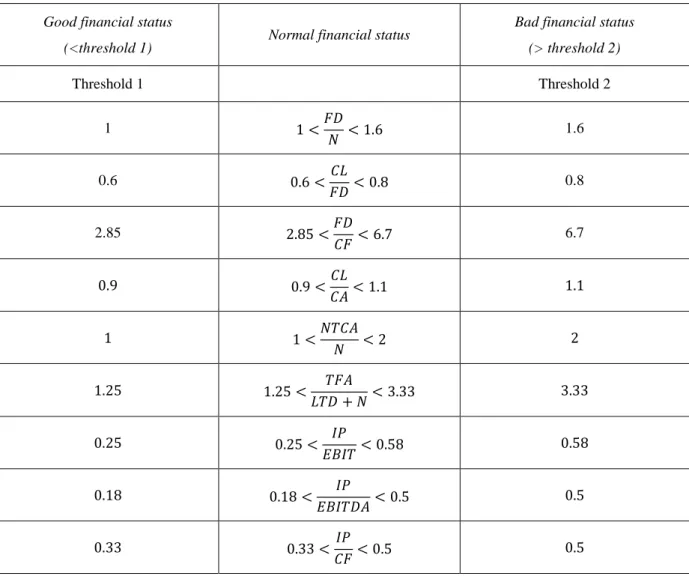
The accounting theory (Bartoli 2006, Brealey and Myers 2001, Fridson 1995, among others) and numerous specialized websites3 suggest - for each financial ratio - specific threshold values which allow us to define when a firm is in a good, normal or bad financial condition, as shown in Table 1.
Table 1 Financial ratios and threshold values Good financial status
(<threshold 1) Normal financial status
Bad financial status (> threshold 2) Threshold 1 Threshold 2 1 1 <𝐹𝐷 𝑁 < 1.6 1.6 0.6 0.6 < 𝐶𝐿 𝐹𝐷< 0.8 0.8 2.85 2.85 <𝐹𝐷 𝐶𝐹 < 6.7 6.7 0.9 0.9 <𝐶𝐿 𝐶𝐴< 1.1 1.1 1 1 <𝑁𝑇𝐶𝐴 𝑁 < 2 2 1.25 1.25 < 𝑇𝐹𝐴 𝐿𝑇𝐷 + 𝑁< 3.33 3.33 0.25 0.25 < 𝐼𝑃 𝐸𝐵𝐼𝑇< 0.58 0.58 0.18 0.18 < 𝐼𝑃 𝐸𝐵𝐼𝑇𝐷𝐴< 0.5 0.5 0.33 0.33 < 𝐼𝑃 𝐶𝐹< 0.5 0.5
3 See, for example, http://www.investopedia.com/articles/investing/080113/understanding-leverage-ratios.asp; http://www.materialitytracker.net/standards/financial-thresholds/; https://www.gov.mb.ca/agriculture/business-and-economics/transition-planning/pubs/ch3-t7-financial-performance.pdf;
https://www.oldschoolvalue.com/blog/valuation-methods/cash-flow-ratios/;
For example, a value of the financial ratio FD/N ranging between 1 and 1.6 denotes a normal financial status of the company. On the contrary, a value below 1 or over 1.6 usually denotes a good or a bad financial condition respectively.
Note that, through the substitution of the threshold values for each financial ratio included in the DEBTINDEX and in the WKNINDEX , it is possible to define the corresponding threshold
values for such two indices and classify the firms according to their degree of indebtedness. More specifically, after estimating the 𝛼 and 𝛿 coefficients, it’s possible to compute the DEBT score and WKN score for every firm. By crossing in a two-way table these two different dimensions we obtain the Composite Indebtedness Index (CI), a classification tool that takes into account both a firm’s indebtedness level and its vulnerability at the same time. Table 2 reports the suggested classification. Let us indicate with +, . (dot) and – the situation in which the considered index is lower than threshold 1, the case in which it is between threshold 1 and threshold 2 and the condition in which it is higher than threshold 2 respectively. If the first subscript refers to the column index and the second one to the row index, then CI++ indicates the best financial status of a firm. 𝑪𝑰∙∙ signals a common indebtedness level of a firm, therefore denoting a normal financial health of a company. The financial health of the firm tends to deteriorate when the firm is highly indebted (𝑪𝑰 − +) or unable to cover the cost of its debt (𝑪𝑰 + −). 𝑪𝑰 ∙− and 𝑪𝑰 −∙ denote a very fragile financial
status. Finally, 𝑪𝑰 − − indicates the situation in which the firm has a relatively high level of debt and it is not able to cover the cost of interests (“pathologic” status).
Table 2 Firm’s financial health classification by CI index
𝑊𝐾𝑁< threshold1 thr. 1<𝑊𝐾𝑁<thr. 2 𝑊𝐾𝑁> threshold2 𝐷𝐸𝐵𝑇<threshold1 𝑪𝑰 ++ optimal 𝑪𝑰 +∙ 𝑪𝑰 + − thr.1<𝐷𝐸𝐵𝑇<thr. 2 𝑪𝑰 ∙+ 𝑪𝑰 ∙∙ normal 𝑪𝑰 ∙− 𝐷𝐸𝐵𝑇>threshold 2 𝑪𝑰 − + 𝑪𝑰 −∙ 𝑪𝑰 − − bad
3.1.2 Robust Estimation of the CI Index
After the pioneering work of Altman (1968), the multivariate approach to failure prediction spread worldwide among researchers in finance, banking and credit risk.
The classical multivariate methods, however, are based on the assumption of normal distribution of variables while financial data are often characterized by asymmetric distribution. For this reason, the traditional multivariate statistical models are not the proper methods to treat such data since the strong asymmetry could bring the researcher to consider too many observations as outliers.
Therefore, to estimate the DEBT and WKN indices I use a robust version of Principal Component Analysis (PCA), through which we obtain the values of the coefficients 𝛼𝑖 and 𝛿𝑖 associated to each financial ratio.
PCA is one of the best known procedures of multivariate statistics. It is a dimension reduction technique which transforms the observed variables into a small number of new variables while retaining as much information as possible. These new variables are linear combinations of the original variables which explain most of the variation in the data, they are uncorrelated and maximize variance, an important information underlying the data. PCA is often the first step of a data analysis, followed by further multivariate analysis like cluster analysis, discriminant analysis, regression or other statistical and/or econometrics techniques.
Let X be a 𝑛 × 𝑝 observed data matrix with n observations and p variables assumed to be correlated. By applying a PCA we obtain a 𝑛 × 𝑝 matrix Y, composed by p new variables, called the principal components (PCs), uncorrelated among them, which are linear combinations of the original variables, according to the following linear transformation: 𝒀 = 𝑿𝑨
where 𝑨 is an orthonormal 𝑝 × 𝑝 matrix whose columns are the eigenvectors of ∑ , the covariance matrix of X. In particular, the first principal component 𝒚𝟏 = 𝑿𝒂𝟏= ∑𝒑𝒌=𝟏𝑎𝟏𝒌𝒙𝒌 is the linear combination of the p original variables xk (column vectors of X) with maximal
variance whose coefficients are given by the first column vector of A; that is the eigenvector
a1 associated to the largest eigenvalue l1 of ∑. Successive p-1 components y2, y3, …, yp are
the linear combinations whose coefficients are given by the successive eigenvectors a2, a3, … ap of ∑ associated to successive eigenvalues l2<l3<…<lp. The variances of the principal
components (PCs) are equal to the li.
Since classical PCA makes use of eigenvalues and eigenvectors of the classical (from sample or population) covariance matrix, this technique is sensitive to outliers and asymmetric
distribution of variables. Various robust alternatives have been proposed in the literature (see Hubert et al. 2005 for a review). Here, in order to robustly estimate the α and δ coefficients of the DEBT and WKN indices, a robust PCA technique - called modified ROBPCA for skewed data - suggested by Hubert et al. (2009) is applied. As in the classical case, these new PCs are
linear combinations of original variables, they are uncorrelated and they are extracted according to their importance in terms of explained variance of the original variables. Hence, the first principal component explains a percentage of variance greater than the second one and so on. The number of extractable PCs is equal to the number of original variables, but eigenvectors and eigenvalues solutions of principal component analysis problem is based on a robust estimate of the covariance matrix of the data (Hubert et al. 2005, 2009).
In real applications, when a PCA analysis is performed, if the original variables have a good degree of correlation, so that a high percentage of the original variance can be explained by few PCs, the first principal component (PC1) is considered a good approximation of the data
matrix X. Indeed, the explained variance, l1, represents a measure of the summary power of
the data given by the first component and it is high if there is a good degree of correlation between the original variables. Usually, a percentage around 50-60 % of explained variance by the first principal component is considered a good value of summary power.
Since accounting data tend to move in the same direction, and more or less proportionately, it is believed that collinearity is always present (Horrigan, 2000). Therefore, I expect the first PC of the two sets of financial ratios to explain a proper percentage of variability, so that 𝐷𝐸𝐵𝑇𝐼𝑁𝐷𝐸𝑋 and 𝑊𝐾𝑁𝐼𝑁𝐷𝐸𝑋 can be properly estimated with the coefficients given by the
eigenvector defining the first robust principal component (RPC1) of the firm’s financial ratios
data matrix.
Once the RPC1 is computed, the combination of the threshold values shown in Table 1 and
the value of the coefficients given by the first eigenvector for each financial ratio included in the DEBTINDEX and in the WKNINDEX, allows us to define the final threshold values for the two
indices: 𝑇ℎ𝑟𝑒𝑠ℎ𝑜𝑙𝑑1𝐷𝐸𝐵𝑇𝐼𝑁𝐷𝐸𝑋 = ∑ 𝛼𝑖 10 𝑖=1 𝑇ℎ𝑟𝑒𝑠ℎ𝑜𝑙𝑑1𝑖 𝑇ℎ𝑟𝑒𝑠ℎ𝑜𝑙𝑑2𝐷𝐸𝐵𝑇𝐼𝑁𝐷𝐸𝑋 = ∑ 𝛼𝑖 10 𝑖=1 𝑇ℎ𝑟𝑒𝑠ℎ𝑜𝑙𝑑2𝑖
𝑇ℎ𝑟𝑒𝑠ℎ𝑜𝑙𝑑1𝑊𝐾𝑁𝐼𝑁𝐷𝐸𝑋 = ∑ 𝛿𝑖 3 𝑖=1 𝑇ℎ𝑟𝑒𝑠ℎ𝑜𝑙𝑑1𝑖 𝑇ℎ𝑟𝑒𝑠ℎ𝑜𝑙𝑑2𝑊𝐾𝑁𝐼𝑁𝐷𝐸𝑋 = ∑ 𝛿𝑖 3 𝑖=1 𝑇ℎ𝑟𝑒𝑠ℎ𝑜𝑙𝑑2𝑖
These threshold values allow us to build the CI index and classify the firms according to their degree of indebtedness (DEBTINDEX) and vulnerability (WKNINDEX).
3.2 Assessment of the probability of default
To evaluate the reliability of the Composite Indebtedness index as early warning signal of financial bankruptcy, a logistic regression technique is applied with the aim to specify the probability of default as a function of a set of explanatory variables. Specifically, the dependent variable is a dichotomous variable that takes value 1 for defaulting firms (the firm is under bankruptcy procedure, it has filed for bankruptcy or it is subject to liquidation in 2011), 0 otherwise (the firm is still active in 2011). In formal terms:
𝑝𝑖,𝑡 = Pr(𝑌𝑖,𝑡 = 1) = 𝐹(𝑥𝑖,𝑡−𝑛𝛽) (1)
where pi,t is the probability that the dependent variable Y=1 for individual firm at time
t=2011, F(_) is the logistic cumulative distribution function, xi,t-n is the set of explanatory
variables thought to affect pi,t with n=1…5; β are the regression coefficients. The explanatory
variables are expressed as follows:
Pr(𝑌𝑖,𝑡 = 1) = 𝐹(𝛽0+ 𝛽1𝐷𝐸𝐵𝑇𝑖,𝑡−𝑛+ 𝛽2𝑊𝐾𝑁𝑖,𝑡−𝑛+ 𝛽3𝑆𝐼𝑍𝐸𝑖,𝑡−𝑛+ 𝛽4𝐴𝐺𝐸𝑖,𝑡−𝑛
+ 𝛽5𝐷_𝑜𝑤𝑛𝑖,𝑡−𝑛+ 𝛽6𝐷_𝑚𝑢𝑙𝑡𝑖,𝑡−𝑛+ 𝛽7𝑃𝑅𝑂𝐷𝑖,𝑡−𝑛+ 𝛽8𝑋_𝑟𝑒𝑔𝑖𝑜𝑛𝑖,𝑡−𝑛 + 𝛽9𝑌_𝑠𝑒𝑐𝑡𝑜𝑟𝑖,𝑡−𝑛)
(2) i = 1… m where i is the ith firm, n=1…5.
In accordance with the general literature on bankruptcy, the model considers the financial structure of the firm. The first two explanatory variables, given by the DEBT and WKN scores computed in the first step of the analysis, take into account the financial health of the firm by measuring both the debt level and its vulnerability. Several works find a significant relation between the financial structure of the firms and their probability of default or exit
from the market (see, among others, Molina, 2005; Hovakimian et al. 2012; Graham et al. 2011; Bonaccorsi di Patti et al. 2014).
The model includes other regressors in order to control for additional non-financial characteristics of the firms, expected to be relevant in determining their probability of default. Both the theoretical and empirical literature suggest that age and size of the firms impact significantly on their performance (for a review, see Klepper and Thompson 2006). More recent studies also analyze the effects of productivity, industrial organization and ownership structure on firm performance (Beck et al. 2006, 2008; Disney et al. 2003; Dunne et al. 1988, 1989; Foster et al. 2006).
Therefore, equation (2) includes additional nonfinancial variables reported hereafter.
The variable SIZEi is computed in terms of a firm’s annual turnover4 and measured in
hundred thousands of Euros.
The variable AGEi is the age of a firm since its foundation.
D_owni is a dummy variable equal to 1 for fully concentrated ownership (unique partner), 0
otherwise (fragmented ownership, several partners). It is a signal of corporate governance since firms in countries with weaker investor protection also have more concentrated ownership (La Porta et al., 1998; La Porta et al., 1999).
D_multi is a dummy variable equal to 1 for multinational firms, 0 otherwise. Multinational
firms have been identified through the analysis of ownership data, by selecting companies owning foreign subsidiaries (ownership share equals 51% by default).
The variable PRODi indicates labor productivity and it is given by value added per employee.
Finally, to take into account the characteristics of the institutional and financial environment in which the firms operate and the specificities of the industrial sectors, I consider both regional dummies and sector dummies as explanatory variables, included in the vectors X and Y respectively. The manufacturing sectors are defined to include firms in the NACE Rev.2 primary codes 10-32. Hence, the model includes 20 regional dummies and 23 sector dummies.
Notice that the two-way Table 2 would also suggest an interaction effect between the DEBT index and the WKN index. This will be explicitly analyzed in section 4.3.
4 In order to measure the size of a firm, different variables could be used like the number of employees, total
assets and turnover. However, the accounting data on “turnover” are more reliable than those on total number of employees reported in the balance sheets, and there are less missing data.
4. An Application to Italian firms
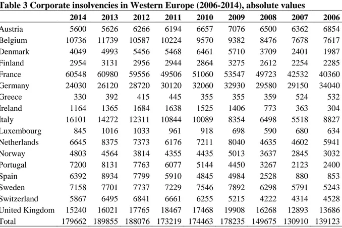
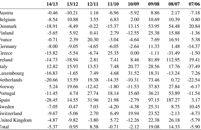
This section illustrates the results of the analysis applied to Italian firms. Despite the easing of the economic situation and the fall in the number of business failures in the Eurozone, the number of corporate insolvencies in Italy is still relatively high and characterized by a positive trend. Table 3 and Table 4 show respectively the absolute values of corporate insolvencies and the year-on year percentage variation in total bankruptcies in Western European countries over the 2006-2014 years. Italy is the only country always characterized by positive percent change in failures over previous year since the 2007-2008 international financial crisis.
As it is illustrated in Figure 1, only Italy and Norway register year-on-year increases in corporate insolvencies 2014. Italy, in particular, shows the highest yearly percentage variation in corporate failures (+12.8 percent).
Table 3 Corporate insolvencies in Western Europe (2006-2014), absolute values
2014 2013 2012 2011 2010 2009 2008 2007 2006 Austria 5600 5626 6266 6194 6657 7076 6500 6362 6854 Belgium 10736 11739 10587 10224 9570 9382 8476 7678 7617 Denmark 4049 4993 5456 5468 6461 5710 3709 2401 1987 Finland 2954 3131 2956 2944 2864 3275 2612 2254 2285 France 60548 60980 59556 49506 51060 53547 49723 42532 40360 Germany 24030 26120 28720 30120 32060 32930 29580 29150 34040 Greece 330 392 415 445 355 355 359 524 532 Ireland 1164 1365 1684 1638 1525 1406 773 363 304 Italy 16101 14272 12311 10844 10089 8354 6498 5518 8827 Luxembourg 845 1016 1033 961 918 698 590 680 634 Netherlands 6645 8375 7373 6176 7211 8040 4635 4602 5941 Norway 4803 4564 3814 4355 4435 5013 3637 2845 3032 Portugal 7200 8131 7763 6077 5144 4450 3267 2123 2400 Spain 6392 8934 7799 5910 4845 4984 2528 880 853 Sweden 7158 7701 7737 7229 7546 7892 6298 5791 5243 Switzerland 5867 6495 6841 6661 6255 5215 4222 4314 4528 United Kingdom 15240 16021 17765 18467 17468 19908 16268 12893 13686 Total 179662 189855 188076 173219 174463 178235 149675 130910 139123 Source: own elaborations on Creditreform data
Table 4 Corporate insolvencies in Western Europe (2006-2014), year-on-year % variation 14/13 13/12 12/11 11/10 10/09 09/08 08/07 07/06 Austria -0.46 -10.21 1.16 -6.96 -5.92 8.86 2.17 -7.18 Belgium -8.54 10.88 3.55 6.83 2.00 10.69 10.39 0.80 Denmark -18.91 -8.49 -0.22 -15.37 13.15 53.95 54.48 20.84 Finland -5.65 5.92 0.41 2.79 -12.55 25.38 15.88 -1.36 France -0.71 2.39 20.30 -3.04 -4.64 7.69 16.91 5.38 Germany -8.00 -9.05 -4.65 -6.05 -2.64 11.33 1.48 -14.37 Greece -15.82 -5.54 -6.74 25.35 0.00 -1.11 -31.49 -1.50 Ireland -14.73 -18.94 2.81 7.41 8.46 81.89 112.95 19.41 Italy 12.82 15.93 13.53 7.48 20.77 28.56 17.76 -37.49 Luxembourg -16.83 -1.65 7.49 4.68 31.52 18.31 -13.24 7.26 Netherlands -20.66 13.59 19.38 -14.35 -10.31 73.46 0.72 -22.54 Norway 5.24 19.66 -12.42 -1.80 -11.53 37.83 27.84 -6.17 Portugal -11.45 4.74 27.74 18.14 15.60 36.21 53.89 -11.54 Spain -28.45 14.55 31.96 21.98 -2.79 97.15 187.27 3.17 Sweden -7.05 -0.47 7.03 -4.20 -4.38 25.31 8.75 10.45 Switzerland -9.67 -5.06 2.70 6.49 19.94 23.52 -2.13 -4.73 United Kingdom -4.87 -9.82 -3.80 5.72 -12.26 22.38 26.18 -5.79 Total -5.37 0.95 8.58 -0.71 -2.12 19.08 14.33 -5.90 Source: own elaborations on Creditreform data
Figure 1 Corporate insolvencies in Western Europe - percentage change 2014/2013
Source: own elaborations on Creditreform 2015
The international comparison highlights significant differences among countries in terms of corporate insolvencies and suggests some distinguishing features of Italian companies, which are worth to analyze. Since firm-level data can provide critical information on firms’ behavior that complements traditional macro analysis, this empirical analysis is based on
-35 -30 -25 -20 -15 -10 -5 0 5 10 15
accounting data of Italian manufacturing firms taken from the Aida Database, published by Bureau Van Dijk. After dealing with missing data,I build up an appropriate database including 31958 Italian small, medium and large manufacturing firms.
The work is carried out on the balance sheet and income statement over the 2006-2010 period in order to analyze the characteristics of firms affecting their probability of default after 5 years, in 2011. An important issue concerns the definition of default. I consider the group membership in 2011, during which some firms failed or were subject to liquidation procedure that brings to failure. Business failure has been defined in many different ways in the empirical literature (Crutzen and Van Caillie, 2008), therefore it is important to clarify the meaning of bankruptcy adopted in this study. Specifically, I focus on companies that have undertaken the juridical procedure of bankruptcy because of permanent financial distress. Therefore, a firm is considered to have defaulted if it is under bankruptcy procedure, if it has filed for bankruptcy or it is in liquidation; I exclude firms with temporary financial problems or companies which have voluntary chosen liquidation for economic opportunity, mergers or acquisition.
The information on the legal status of the firms with respect to bankrupt procedures has been collected from the AIDA database.
By applying the default definition provided, the work focuses on two groups of firms: defaulting firms and non-defaulting firms. The composition of the sample is provided in Table 5.
Table 5 Sample Composition, 2010
Total n. of firms Defaulting Firms Non-defaulting firms Number Percentage Number Percentage Number Percentage
Total 31958 100 1856 5.81 30102 94.19 Geographical Area North 23659 74.03 1225 5.18 22419 94.82 Center 5038 15.76 367 7.28 4671 92.72 South 3261 10.20 264 8.09 2997 91.91 Turnover 2-10 million euros 21246 66.48 1207 5.68 20039 94.32 10-50 million euros 8226 25.74 271 3.29 7955 96.71 >50 million euros 2486 7.78 378 15.2 2108 84.8 Age <15 11049 34.57 882 7.98 10167 92.02 16-24 7550 23.62 371 4.91 7179 95.09 25-32 6342 19.84 271 4.27 6071 95.73 >33 7017 21.96 332 7.35 6685 92.65
Source: own elaborations on Aida database
The manufacturing firms included in the sample operate in different geographical areas, in different sectors and they significantly differ in size. Since both large companies and SMEs are considered, in order to mitigate the effect of firm size on selected variables, I first consider large, medium and small enterprises separately; then divide each financial variable by the average turnover of the corresponding group and, finally, build up the financial ratios. As mentioned above, the full sample includes 31958 firms. The defaulting firms’ group includes 1856 firms failed in 2011 and represents 5.81% of the firm population, while the non-failed group consists of 30102 companies representing 94.19% of the total. With reference to the geographical area in which the firms are located, the population includes 23644 firms in the North, 5038 in the Center and 3257 in the South of Italy. The distribution of failed firms among the different geographical areas mirrors the composition of the whole population. Most of defaulting firms, at least in absolute terms, are concentrated in the North (1225), while default firms in the Center and in the South of the country are 367 and 264 respectively. Looking at percentage values, the distribution of the two groups of firms shows a prevalence of default firms in the South of Italy.
Table 5 also shows the composition of the sample with respect to firm size and age. As mentioned above, as measure of size I consider the annual turnover, one of the parameters adopted by the Basel II Committee to define SMEs, while age is in terms of years of activity
since firm foundation. Data show a relatively higher concentration of bankruptcies among SMEs and young firms.
In Europe, the distribution of insolvency among the different branches of the economy can vary considerably. Southern European countries usually register large numbers of defaulting firms in manufacturing sectors. In 2010, for example, Italy registers 24.1 percent of default firms belonging to manufacturing sectors, a value above the European average.
Table 6 shows the percentage of corporate insolvencies across the manufacturing sectors, identified following the NACE Rev.2 classification and structured, for a descriptive purpose, following the Intermediate level SNA/ISIC-A*38 aggregation.
Within the manufacturing industry, the incidence of failure is relatively higher in the sectors of motor vehicles and transport equipment (8.44%), repair and installation of machinery and equipment (8.25%), followed by manufacture of wood, paper products and printing (7.42 %). The manufacture of chemical and chemical products and the manufacture of pharmaceuticals, medicinal, chemical and botanical products show the lowest percentages of corporate failures, registering 2.70% and 2.91% of insolvencies respectively.
Table 6 Percentage of corporate insolvencies by sector, year 2010 NACE Rev.2 code Sector Description N of defaulting firms Total N of firms % of corporate insolvencies 10, 11, 12
Manufacture of food products, beverage and tobacco products
117 2855 4.10
13, 14, 15
Manufacturing of textiles, apparel, leather and related products
265 3953 6.70
16, 17, 18
Manufacture of wood, paper products and printing 174 2345 7.42 19 Manufacture of coke and refined petroleum
products
5 155 3.23
20 Manufacture of chemical and chemical products 38 1406 2.70 21 Manufacture of pharmaceuticals, medicinal,
chemical and botanical products
9 309 2.91
22, 23 Manufacture of rubber and plastics products, and other non-metallic mineral products
234 3750 6.24
24, 25 Manufacture of basic metals and fabricated metal products, except machinery and equipment
408 6737 6.06
26 Manufacture of computer, electronic and optical products
60 1096 5.47
27 Manufacture of electrical equipment 70 1564 4.48
28 Manufacture of machinery and equipment n.e.c. 217 4670 4.65 29, 30 Manufacture of motor vehicles, trailers and
semi-trailers Manufacture of transport equipment
83 983 8.44
31, 32 Manufacture of furniture Other manufacturing; repair and installation of machinery and equipment
176 2134 8.25
4.1 Analysis of the financial health of Italian manufacturing firms through the CI index In this paragraph the results obtained by applying the Robust PCA analysis to the Italian case are firstly presented and discussed, and then the classification obtained through the estimated
CI index is illustrated.
Notice that, to estimate DEBT e WKN coefficients, the Robust PCA algorithm has been applied to average values of financial ratios over the 2006-2010 years in order to increase the stability and the reliability of such financial indices.
After applying the Robust PCA method, I obtain new RPCs variables that are linear combination of original financial ratios, they are uncorrelated and maximize variance. The percentage of variance explained by each Robust PC is computable from the robust eigenvalues given by the Robust PCA algorithm (Appendix, Table A.1).
As expected, the first robust principal component represents the most important dimension in explaining changes of financial conditions since it explains 72.5% of the total variance. Thus, I retain RPC1 to estimate the coefficients 𝛼𝑖 for 𝐷𝐸𝐵𝑇𝐼𝑁𝐷𝐸𝑋:
𝑫𝑬𝑩𝑻𝑰𝑵𝑫𝑬𝑿 =0.9192𝐹𝐷 𝑁 + 0.0045 𝐶𝐿 𝐹𝐷+ 0.0885 𝐹𝐷 𝐶𝐹+ 0.0254 𝐶𝐿 𝐶𝐴+ 0.3706 𝑁𝑇𝐶𝐴 𝑁 + 0.0657 𝑇𝐹𝐴 𝐿𝑇𝐷+𝑁
With reference to financial ratios included in the WKNINDEX, the first robust principal
component is also the most important dimension in explaining changes in sustainability of firms’ debt. It explains 56.2% of the total variance of the financial ratios (Appendix, Table A.2). As for 𝐷𝐸𝐵𝑇𝐼𝑁𝐷𝐸𝑋, the coefficients 𝛿𝑖 for 𝑊𝐾𝑁𝐼𝑁𝐷𝐸𝑋 are estimated by retaining only RPC1: 𝑾𝑲𝑵𝑰𝑵𝑫𝑬𝑿 = 0.1572 𝐼𝑃 𝐸𝐵𝐼𝑇+ 0.2515 𝐼𝑃 𝐸𝐵𝐼𝑇𝐷𝐴+ 0.9550 𝐼𝑃 𝐶𝐹
Using the threshold values shown in Table 1, I can define the final threshold values for both DEBTINDEX and WKNINDEX, derive the CI index and then classify the firms according to their
degree of indebtedness and vulnerability:
𝑇ℎ𝑟𝑒𝑠ℎ𝑜𝑙𝑑1𝐷𝐸𝐵𝑇𝐼𝑁𝐷𝐸𝑋 = ∑7𝑖=1𝛼𝑖 𝑇ℎ𝑟𝑒𝑠ℎ𝑜𝑙𝑑1𝑖=1.65 𝑇ℎ𝑟𝑒𝑠ℎ𝑜𝑙𝑑2𝐷𝐸𝐵𝑇𝐼𝑁𝐷𝐸𝑋 = ∑7𝑖=1𝛼𝑖 𝑇ℎ𝑟𝑒𝑠ℎ𝑜𝑙𝑑2𝑖=3.06
𝑇ℎ𝑟𝑒𝑠ℎ𝑜𝑙𝑑1𝑊𝐾𝑁𝐼𝑁𝐷𝐸𝑋 = ∑3𝑖=1𝛿𝑖 𝑇ℎ𝑟𝑒𝑠ℎ𝑜𝑙𝑑1𝑖=0.29
𝑇ℎ𝑟𝑒𝑠ℎ𝑜𝑙𝑑2𝑊𝐾𝑁𝐼𝑁𝐷𝐸𝑋 = ∑3𝑖=1𝛿𝑖 𝑇ℎ𝑟𝑒𝑠ℎ𝑜𝑙𝑑2𝑖=0.69
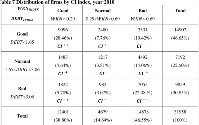
Table 7 illustrates the distribution of the Italian manufacturing firms in 2010 according to this classification.
Table 7 Distribution of firms by CI index, year 2010 𝑾𝑲𝑵𝑰𝑵𝑫𝑬𝑿 𝑫𝑬𝑩𝑻𝑰𝑵𝑫𝑬𝑿 Good 𝑊𝐾𝑁< 0.29 Normal 0.29<𝑊𝐾𝑁<0.69 Bad 𝑊𝐾𝑁> 0.69 Total Good 𝐷𝐸𝐵𝑇<1.65 9096 (28.46%) 𝑪𝑰 ++ 2480 (7.76%) 𝑪𝑰 +∙ 3331 (10.42%) 𝑪𝑰 + − 14907 (46.65%) Normal 1.65<𝐷𝐸𝐵𝑇<3.06 1483 (4.64%) 𝑪𝑰 ∙+ 1217 (3.81%) 𝑪𝑰∙∙ 4492 (14.06%) 𝑪𝑰 ∙− 7192 (22.50%) Bad 𝐷𝐸𝐵𝑇>3.06 1822 (5.70%) 𝑪𝑰 − + 982 (3.07%) 𝑪𝑰 −∙ 7055 (22.08 %) 𝑪𝑰 − − 9859 (30.85%) Total 12401 (38.80%) 4679 (14.64%) 14878 (46.55%) 31958 (100%) Source: own elaborations on Aida database
According to the classification based on the CI index, the percentage of Italian manufacturing firmsin the best financial status 𝑪𝑰 ++ is 28.46%; these firms have a low level and a good
sustainability of debt. 22.08% of firms are classified in the worst financial status 𝑪𝑰 − −; these firms are characterized by a high level of debt and a bad sustainability of the debt, therefore the risk to fail is expected to be high.
4.2 Econometric Results
Table 8 shows the logistic regression estimates for different lengths of the reference period, in particular for 1, 2, 3, 4 and 5 years before failure.
Those variables performing well in the latest year before failure will not necessarily perform well in the other years prior to failure. Some variables, however, can play an important role in more than one regression given the long run nature of some factors leading to failure.
Given the non-linearity of the first-order conditions with respect to parameters, a solution of numerical approximation is adopted that reaches the convergence after five reiterations. Table 8 reports the maximized value of the log-likelihood function for all the regressions.
LR Chi-square (50) is the asymptotic version of the F test for zero slopes.The p-value allows the rejection of the null hypothesis that all the model coefficients are simultaneously equal to zero. Therefore, the model as a whole is statistically significant. To avoid the risk of multicollinearity among variables, the computed bivariate correlation test has been carried
out. It does not reveal any linear relation among variables. To further corroborate this result two additional measures, namely the ‘‘tolerance’’ (an indicator of how much collinearity a regression analysis can tolerate) and the VIF (variance inflation factor, an indicator of how much of the inflation of the standard error could be caused by collinearity) have been computed. Since both measures are close to 1 for the considered variables, any multicollinearity can be excluded.
Turning to the analysis of the estimates, the empirical findings show that both the DEBT score and the WKN score are statistically significant at 1% level with the expected positive sign. An increase in firm’s debt level and/or in its unsustainability significantly increases the probability of default.
Table 8 also reports the odds ratio of the logistic regression, which coincides with the exponential value of the estimated parameters. Considering one year prior to failure (2010), for a unit increase in the DEBT score, the odds of bankruptcy increases by 44%, holding the other variables constant. Likewise, a unit increase in the WKN score raises the odds by 67.9%. In other words, firms that are exposed to high debt are more than 1.44 times (e0.365) likely to fail than the other firms; firms with an unsustainable debt are more than 1.68 times (e0.518) likely to go to bankrupt than the other firms.
From these results it is clear that the level of indebtedness and its nature are important factors in explaining firms' default risk. Interestingly, both indices enter with the highest coefficients in all the regressions, that is for different lengths of the reference period. Moreover, the coefficient associated to the vulnerability of debt is always greater than that related to the absolute level of debt5. Hence, it is certainly true that total amount of debt and its composition signal the financial health of the company, but the capacity/potential of the firm to sustain such debt is a more important factor to consider in firms’ creditworthiness evaluation. In this context, an early warning signal of default risk would assume a pivotal role in the adoption of effective reorganization procedures.
With reference to the other explanatory variables, firm size enters with negative sign at 10% level of significance, therefore larger companies would face lower probability of default. Note, however, that firm size is not significant when we consider long period prior to failure. Age enters at 1% level with negative sign, suggesting that younger firms are more likely to go to bankruptcy than larger companies. These results confirm previous empirical findings on the impact of age and size on firm performance (European Central Bank, 2013; Hurst and
5
Note that the relatively higher coefficient associated to the variable WKN cannot be ascribed to scale differences because, as mentioned above, financial ratios have been standardized.