MODELING THE RELATIONSHIP BETWEEN PERCEIVED NEIGHBOURHOOD CHARACTERISTICS AND ADULT
HOSPITALIZATION FREQUENCIES FROM A CROSS-SECTIONAL STUDY P. Bellini, D. Lo Castro, F. Pauli1
1. INTRODUCTION
Interest in the effects of neighbourhood or local area characteristics on health status and outcomes has increased in recent years; the feeling is that the context in which people live, as well as personal characteristics, affects their well-being and quality of life. Identifying which neighbourhood qualities and characteristics are more important to health is then a crucial issue not only for a better under-standing of the connection between health and place, but also to assess health status of communities and to inform future health intervention strategies (Berk-man and Kawachi, 2000).
Statistical modelling plays a central role in dealing with this issue. Generally speaking, one needs data on health status and other relevant characteristics of individuals and neighbourhoods. A statistical model is then used to shed light on the interrelationships among the quantities involved. Several studies of local urban area effects have been conducted focusing on the impact of neighbour-hood characteristics on health outcomes after adjusting for individual status. They differ according to the population considered, the (response and explana-tory) variables and the statistical models involved. The statistical approach used depends on the characteristics of the data and the specific questions to be an-swered; examples include: various (G)LM (Bowling et al., 2006; Wen et al., 2006; Wilson et al., 2004; Abada et al., 2007; Propper et al., 2007) multilevel regression (Pickett and Pearl, 2001; Wen et al., 2007; O’Campo, 2003), graphical models (Rajulton and Niu, 2005), spatial models (Chaix et al., 2005 and 2006) structural equation (Weden et al., 2008; Li and Chuang, 2009). A more comprehensive dis-cussion of the conceptual framework behind these models can be found in Bel-lini et al. (2008).
In this paper the neighbourhood qualities we take into consideration are the perceptions that each individual has of a number of neighbourhood
tics. These are included in the model as individual rather than contextual variables (quantities computed for each neighbourhood and then associated to each indi-vidual living in that neighbourhood). Using indiindi-vidual perceptions about the neighbourhood may be seen as a limitation of the present study, when they should, in fact, be regarded as measures with error of the neighbourhood quality. Using the perceptions, however, may also be a strength for two main reasons. First, since conclusions on neighbourhood effect are sensitive to the neighbour-hood definition that is adopted (Flowerdew et al. (2008)) – to the extent that spu-rious results may be found (Spielman and Yoo (2009)) – the fact that we avoid choosing a – necessarily arbitrary – specific definition leads to more robust re-sults. In particular, geographic or administrative boundaries – which are the most common choices – may not be the appropriate definition when dealing with characteristics related to social interactions (Diez Roux, 2001); in this case the ‘perceived’ neighbourhood (which is the definition implicitly used here) may be a more appropriate choice. Second, it may be argued that the effect of the neighbourhood is not merely the result of its objective qualities, but also depends on subjective factors (this may be true in particular for social characteristics, but, even if we consider an eminently objective feature such as pollution, its effect on an individual depends on his personal degree of exposure). The connection be-tween neighbourhood perceptions and health has already been discussed in the literature, and a variety of perceived aspects of the neighbourhood is considered by the various authors. Broadly speaking one may distinguish perception of the physical (or environmental) characteristics of the neighbourhood and perceptions related to the social capital; the latter may concern problems due to (anti-)social behaviour on the negative side and to social cohesion on the positive side. Some authors aggregate individual perception at the neighbourhood level and use the result as a contextual variable finding a significant effect (Pampalon et al., 2007; Wen et al., 2006). Pampalon and co-authors explicitely discuss the issue of whether aggregated individual perceptions are a suitable contextual variable. Per-ceptions of physical and social characteristics have also been used as individual (non contextual) variables. They were found to have a significant effect on health in Glasgow (UK) (Ellaway et al., 2001); in Hamilton (Canada) (Wilson et al., 2004) and among British over age 65 (Bowling et al., 2006). In particular, the signifi-cance of the perception of physical problems in the neighbourhood is empha-sized by the cited authors. Perceptions were significantly associated to asssess-ment of depression in Schaefer-McDaniel (2009). In previous studies a significant effect of social cohesion on adolescent health has been estimated (Abada et al., 2007). Other authors estimated a more complex relationship involving an interac-tion between individual trust and a contextual variable measuring community trust (Subramanian et al., 2002). Finally, using L.A.FANS data, it was found that social capital (as measured by the variables called closeknit, safe and neigh.satisf in Table 2) has a significant effect on self-reported health in poor and very poor neighbourhoods (Shin et al., 2006).
On the response variable side we choose to consider the number of zations as the health outcome. The effect of neighbourhood quality on
hospitali-zation frequency has been explored relatively rarely; evidence has been found of a negative relationship between socio-economic status of the neighbourhood and hospitalization frequency (Booth and Hux, 2003; Taylor et al., 2006). This is un-surprising since hospitalization frequency in the general population is difficult to model due to the high proportion of zeroes generally observed. In this work we try to show that this inconvenience can be successfully dealt with through suit-able models. Moreover, we prefer number of hospitalizations rather than the main alternatives, number of visits to a physician and perceived (self-assessed) health status, because the former is a more objective measure of health status with respect to perceived health and also, to a lesser extent, with respect to the number of visits to a physician. In prospect, it may also be interesting to model both hospitalizations and visits in a bivariate setting. A further alternative meas-ure of health status would be having been diagnosed as suffering from specific pathologies; such a choice, however, would be appropriate for a study devoted to specific pathologies rather than a study concerned with general health.
The fact of using perception of the neighbourhood quality as explanatory vari-ables is one more reason to prefer an objective measure of health conditions as the response variable: any association of self-reported health status to perceived neighbourhood quality may be spurious, since it may be driven by the overall atti-tude of the respondent (Pampalon et al., 2007; Weden et al., 2008). Moreover, it is worth saying that our purpose is not to infer a causal relationship between neighbourhood characteristics and health – the cross-sectional nature of the data that we use would not consent that, anyway – but merely to develop a statistical model for the association between the two quantities.
Bearing in mind all the above, we need, from a modelling point of view, an asymmetric model for count data (i.e., for integer response). A generalized linear model with Poisson response would be the most common choice in such a con-text. However, the relatively unusual choice of hospitalization data leads to a complication: in fact, the Poisson model proves to be inadequate mainly because of a high proportion of zeroes, which cannot fit into a Poisson assumption. This is a relatively common issue in applied statistics literature, particularly in epidemi-ology, and the typical solution is to replace the Poisson assumption with the Zero-inflated Poisson or the Negative-Binomial distribution (Böhning et al., 1999; Hur et al., 2002; Lee et al., 2006), in the context of urban studies, on the contrary, this option is seldom, if ever, taken. Because we consider hospitalization data, however, we could not ignore the issue, and we want to stress that this has proved relevant in interpreting the results.
2. DATA
We consider the data collected within the Los Angeles Family and Neighbour-hood Survey (L.A.FANS) (Peterson et al., 2004), which has already been exploited in the literature. The Los Angeles Family and Neighbourhood Survey (L.A.FANS) is a panel study performed by the RAND corporation. In L.A.FANS
a representative sample of households in Los Angeles County has been inter-viewed in two waves (2000-2001 and 2004-2005). The study is aimed at offering a better understanding of neighbourhood effects. For this reasons questionnaires ask for informations concerning neighbourhood characteristics and the random sample is stratified by neighbourhood – 65 neighbourhood (census tracts) in L.A. county were considered. Also, poor neighbourhoods and families with children are oversampled.
In the first wave, which is considered here, 3085 households were sampled (of which, 777 cases were households without children and 2308 with children) and for each of them interviews were made to a Randomly Selected Adult (RSA) and, if the household had children, a Randomly Selected Children (RSC), a Sibling (SIB) and the Primary Care Giver (PCG); in the end 2620 adults, 3161 children (2001 RSC and 1160 SIB) and 2044 caregivers completed the interview (see Fig-ure 2.3 and Table 2.8 in Peterson et al., 2004). In this work we do not consider family issues, so we consider only answers from the 2537 RSA interviewed who responded to the question concerning hospitalizations.
In Table 1 we briefly describe the personal characteristics taken under con- sideration. In Table 2 we list variables describing the characteristics of the neighbourhood as perceived by the respondent (which are the only information on neighbourhood considered here). Such variables are related to social re-sources availability (social cohesion and trust, informal social control), envi-ronmental stressors (safety) and general satisfaction with neighbourhood. The responses on these topics are highly dependent, so it is advisable to build indi-cators which sum up subsets of them rather than to use all of them as covari-ates. A similar approach can be found in the literature too (Ellaway et al., 2001; Wilson et al., 2004; Subramanian et al., 2002; Shin et al., 2006): a number of questions are asked related to the perceived aspects of the neighbourhood and the answers are usually collapsed in a few indicators (among the cited studies only that by Wilson et al. (2004) is different on this respect in that respondents were asked open ended questions on likes and dislikes concerning the neighbourhood, also in this case, however, they were eventually collapsed in a few indicators). In this work, attempts have been made, unsuccesfully, at using data driven techniques such as cluster analysis to define indicators, eventually we defined indicators heuristically.
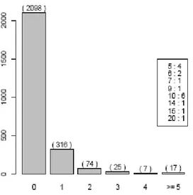
The frequency distribution of the response variable is depicted in Figure 1 where it is seen that 82% of respondents reported no hospitalization. This is to be expected working with hospitalization data referred to the general population; it is worth noting that it does not inform us whether an excess of zeroes exists with respect to the traditional Poisson distribution assumption. In fact, we are not interested in the marginal distribution of the response variable, which is repre-sented here, but on the conditional distributions estimated by the model. Suitabil-ity of a zero-inflated distribution will emerge from an analysis of the results of the fit.
Figure 1 – Frequency distribution of the number of hospital admissions for RSA (Randomly
Se-lected Adult), in the box the frequencies of number of hospitalizations of RSA with 5 or more hos-pitalizations (in addition, 82 missing observations are present).
TABLE 1
Relevant variables in L.A.FANS. Body mass index is the ratio between self reported weight (in kg) and squared height (in meters); per capita income is given by the total income divided by the number of cohabitants
(it is to be noted that this variable is censored since it is the sum of censored variables) Name n. levels description (levels, 1-level for dichotomic)
nhosp num Number of hospital admissions in the 24 months preceding interview (mean: 0.33; min: 0; max: 20) age num Age of respondent (mean: 41.13; min: 18; max: 89)
bmi num Body mass index (BMI) of respondent (mean: 26.25; min: 17.48; max: 40.39) proincome num Per capita income within family (mean: 14157.08; min: 0.00; max: 190000.00) gender 2 gender (male)
race 5 race (latino, white, black, asian/pacific, native/other)
empl 4 employment status (unemployed (not recent), never employed, unemployed (recent), employed) welfareinc 2 income from welfare (yes)
house 3 status house (owned, rented, other) edu 3 education (less, high, college)
marstatus 4 marital status (married, living with partner, neither, both)
rsoc 2 having a regular source of care different than relatives and friends (yes) res.stab 2 residential stability (moved since less than 5 years)
Previous diagnosesa
cld 2 diag. of chronic lung disease excweight 2 diag. of excess weight depress 2 diag. of major depression cancer 2 diag. of cancer/malignancy emotional 2 diag. of emotional problems hbp 2 diag. of high blood pressure diabetes 2 diag. of diabetes ha 2 diag. of heart attack chd 2 diag. of coronary heart disease artrrheum 2 diag. of arthritis or rheumatisms asthma 2 diag. of asthma
mentalloss 2 diag. of loss of mental ability learndis 2 diag. of learning disorder
TABLE 2
Relevant variables related to neighbourhood in L.A.FANS Name n. levels description (levels, 1-level for dichotomic)
Variables concerning informal social controla hangout 2 neighbours do something if kid hangs out
graffiti 2 would do something if kid does graffiti Disresp 2 would scold kid if showing disrespect inf.soc.ctrl index of informal social controlb
Variables concerning social cohesionc closeknit 2 this is a close knit neighbourhood
willhelp 2 people are willing to help neighbours getalong 2 neighbours generally get alongd
sharevalues 2 people in neighbourhood share same valuese trusted 2 people in neighbourhood can be trusted cohes.trust index of social cohesion and trustf
Variables concerning safety in neighbourhood
safe 4 how safe is to walk around alone (1=completely safe to 4=extremely dangerous) robbed 2 household has been robbed or suffered vandalism in the neighbourhood (0=no to 1=yes)
Other variables describing neighbourhood
neigh.satisf 5 degree of satisfaction with the neighbourhood (1=very satisfied to 5=very dissatisfied)
a All but the last are coded as 1=‘very likely’; 2=‘likely’; 3=‘unsure’; 4=‘unlikely’; 5=‘very unlikely’ in the original coding, they are dichotomized as ‘unlikely’=0=‘unlikely’ or ‘very unlikely’; ‘likely’=1=‘very likely’ or ‘likely’; response ‘unsure’ was ignored as a missing value.
b The (non weighted) sum of the dichotomized variables concerning informal social control.
c All but the last are coded as 1=‘strongly agree’; 2=‘agree’; 3=‘unsure’; 4=‘disagree’; 5=‘strongly disagree’ in the original coding, they are dichotomized as ‘Agree’=1=‘strongly agree’ or ‘agree’; ‘Disagree’=0=‘disagree’ or ‘strongly disagree’; response ‘unsure’ was ignored as a missing value.
d Variable has been given the opposite sense here than in L.A.FANS questionnaire (original question was ‘neighbours generally don’t get along’).
e Variable has been given the opposite sense here than in L.A.FANS questionnaire (original question was ‘people in neighbour-hood don’t share same values’).
f The (non weighted) sum of the dichotomized variables concerning social cohesion and trust.
3. METHODS
Conceptually, we use an asymmetric model involving the number of hospitali-zations occurred in the 24 months preceding the interview (Y) as the response variable and a selection of possible determinants as the explanatory variables (xh).
We consider generalized additive models (GAM) to analyse separately the, possi-bly non linear, effect of each covariate on the response. Non linear contributions are estimated by spline functions whose degree of smoothness is decided by gen-eralized cross validation.
Being Y a frequency, the traditional model for it would be based on the Pois-son distribution ( ) ! i y i i P Y y e y (1)
and on the logarithmic link function between the parameter and the linear predic-tor, so that, if xh,i (with h= 1, ..., H and i=1, ..., n) is the observed value of the h
covariate on the i-th unit,
0 , , log( ) ( ) s l i h h i h h i h H h H g x x
(2)where gh() are spline functions. The effects of covariates indexed in Hs
1,..., H are modeled non linearly, those indexed in Hl 1,..., H are modelled
linearly (Hs Hl= and Hs Hl 1,..., H).
The Poisson assumption may be too restrictive for real count data, a common extension is the Zero Inflated Poisson model (Lam et al., 2006) that is, one as-sumes that
i i i
Y Z W (3)
where Zi is 0 with probability i and 1 with probability 1-i and (Wi|Zi=1)
Pois-son (i), meaning that
( ) ( 0) (1 ) ! i y i i i i P Y y I y e y (4)
Covariates may affect either the parameter i and/or the parameter i through
suitable link functions, the logistic and the logarithm functions respectively in this work, so we get the two linear predictors
0 . . logit( ) ( ) s l i h h i h h i h H h H g x x
(5) 0 . . log( ) ( ) s l i h h i h h i h H h H g x x
(6)where all symbols are to be interpreted analogously to equation (2) (Hs Hl =
and Hs Hl = , while the other couples may have, pairwise, non empty
in-tersections). Lam et al. (2006) recently proposed a method based on approximat-ing the smooth functions by piecewise linear functions and on usapproximat-ing the sieve maximum likelihood approach to obtain estimates to perform a semiparametric analysis within a ZIP assumption. We prefer the approach of Rigby and Stasi-nopulos (2005), which is based on the spline functions representation of smooth functions and the penalized likelihood approach to obtain estimates. This latter approach is in fact, to our knowledge, more widely used and tested. In practice, estimation is made using the package gamlss (Stasinopulos and Rigby, 2007) in R (R Development Core Team, 2005).
The use of a ZIP model implies greater flexibility but, on the other side, inter-pretation of results is a bit harder. In fact, in a ZIP model the total effect of a variable, say xh*, on the expected number of hospitalizations is a combination of
-1 0 . . ( | ) (1 ) 1 logit ( ) s l i i i i h h i h h i h H h H E Y g x x
x 0
.
. exp ( ) s l h h i h h i h H h H g x x . (7)The result of such a combination is not obvious and, moreover, the shape of the function s(xh*)=E(Y|xh*,x-h*), also depends (due to the non linearity of the link
functions) on the values of the other covariates. For this reason, in order to get a glance of the dependence of Y on xh we compute E(Y|xh*,x-h*) for a grid of values
of the effect of xh*. In practice, we compute for all observed units i the quantities
. . \ * \ * ( ) s l i h h i h h i h H h h H h v g x x
(8) . . \ * \ * ( ) s l i h h i h h i h H h h H h v g x x
(9)and consider, for some values q[0, 1], fixed empirical q-quantiles v([qn]) and v([qn])
(where [qn] is the integer part of qn). These values are then substituted in equation (7) to get * -1 * 0 * * * * [ ] ( ) [1 logit ( ( *) ( ) ( *) )] s l q h H h h H h h qn s x I h g x I h x v exp( 0 IHs( *)h gh*(xh*) IHl( *)h h*xh* v[ ]qn ) (10)
where IK(k) is an indicator function which is one if kK and zero otherwise.
An alternative model one may consider is the Negative Binomial model, which is more flexible than the Poisson model (but not nested), the distribution of Y is then ( 1/ ) ( 1/ ) ( ) ( ) ( 1) (1/ ) ( 1) i y i i i i y i i i y P Y y y (11)
in which log(i)=0 and
0 . . log( ) ( ) s l i h h i h h i h H h H g x x
(12)is the linear predictor for .
Model comparison for variable selection is based on standard criteria: Akaike Information Criterion (AIC), Bayesian Information Criterion (BIC) and residual deviances comparison.
To assess model adequacy we check normality of the randomized residuals, that is, the quantities
ˆ ˆ
(1 ) ( 1) ( )
i i i i i i i
r u F y u F y (13)
where ui are independent and identically distributed uniform random variables on
[0,1], ˆF is the Poisson, ZIP or NB distribution function with parameters equal to the estimated values (so for example in the ZIP case F yˆ ( )i F( ; , )y ˆi ˆi where F
is the d.f. of the ZIP). In any case randomized residuals are, if the model is cor-rect, normally distributed.
4. RESULTS
In section 4.1 we report the results we got using ZIP model, in section 4.2 we briefly explore whether a simpler model – Poisson or Negative Binomial – fits well to the data.
4.1. ZIP model
Our model selection strategy is first to choose the most relevant among physiological characteristics of the individual, then among the socioeconomic and sociodemographic ones and finally among those concerning the neighbourhood. Choice of candidate variables for inclusion is based on previous experiences ac-crued in the literature.
In Table 3 we report the AIC, BIC and deviance values relevant for model comparisons. The procedure is incremental; in the i-th line we compare by AIC and BIC the current model, which involves all the variables selected up to step i, and the model obtained applying the i-th modification: this is actually applied (and hence the current model for step i+1 is the one resulting from the modifica-tion) if it leads to a better AIC or BIC value than the simpler model and if the co-efficient of the variable which is added is significantly different from zero at 5% level. It must be kept into account the fact that each variable has missing values for different units, so in order to do a fair comparison we must estimate both models on the same dataset (the largest one having no missing observations for the relevant variables). (It is to be noted that the inclusion of the quantities in Ta-ble 3 corresponds to the inclusion of a set of dummy variaTa-bles when the quantity is a categorical variable; in this case the selection of significant coefficients may lead to the inclusion of only part of these dummy variables, that is, to an alterna-tive definition of the factor levels.)
The ZIP model we start from (M0) includes the main physical characteristics:
age, body mass index (BMI) and gender; in particular, it includes a non linear function of age and a dummy variable for gender in both linear predictors, while a non linear function of BMI enters only the linear predictor for .
TABLE 3
Pairwise comparisons of ZIP models for successive additions of variables from base model M0 (including age, gender and BMI) to final model M1 (including variables in bold face in the table)
Cathegories in the CF AIC BIC Deviance
n d.f. w/out with w/out with w/out with
+age+gender+BMI 2343 16 - 3061.12 - 3153.3 - 3029.1 +D1 2336 35 3058.63 2868.83 3150.7 3070.3 3026.6 2798.8 +D2 2336 28 2868.83 2992.48 3070.3 3153.6 2798.8 2936.5 +D3 2336 21 2992.48 2989.2 3153.6 3110.1 2936.5 2947.2 +race 2336 25 2989.2 2920.66 3110.1 3064.6 2947.2 2870.7 Physical characteristics -g(age)+age 2336 21 2920.66 2925.2 3064.6 3046.1 2870.7 2883.2 +g(proincome) 2295 23 2875.82 2870.47 2996.3 3002.5 2833.8 2824.5 +empl 2295 25 2870.47 2819.7 3002.5 2963.2 2824.5 2769.7 +welfare.inc 2283 26 2797.18 2797.15 2940.5 2946.2 2747.2 2745.2 Socioeconomic characteristics +house 2291 29 2818.09 2820.5 2961.5 2986.9 2768.1 2762.5 +edu 2265 27 2791.33 2790.53 2934.5 2945.1 2741.3 2736.5 +marstatus 2265 28 2790.53 2777.46 2945.1 2937.8 2736.5 2721.5 Sociodemographic characteristics +rsoc 2261 29 2776.3 2774.16 2936.6 2940.1 2720.3 2716.2 +res.stab 1712 29 2120.43 2119.75 2272.9 2277.7 2064.4 2061.7 +safety 1450 30 1908.62 1899.82 2061.7 2058.2 1850.6 1839.8 +inf.soc.ctrl 1302 31 1690.83 1689.96 1846 1850.3 1630.8 1628.0 +cohes.trust 1118 31 1503.48 1504.58 1654.1 1660.2 1443.5 1442.6 +i.s.c & c.t. 1046 32 1404.09 1397.59 1552.7 1556.1 1344.1 1333.6 +neigh.satisf 1046 40 1397.59 1380 1556.1 1578.1 1333.6 1300.0 Neighbourhood -I 1046 31 1380 1368.99 1578.1 1522.5 1300 1307
D1: set of all diagnoses variables (see Table 1);
D2: set of those diagnoses which are less correlated with age (excess weight, depression, cancer, emotional disorder, chronic lung disease, asthma, loss of mental ability, learning disorder);
D3: set of those diagnoses which are significant in the model (that is, excess weight, depression, cancer, emotional disorder and chronic lung disease);
-g(age)+age stands for the replacement of the non linear contribution of age with a linear one;
i.s.c & c.t stands for the set of those variables related to informal social control and cohesion trust (listed in Table 2) having an estimated coefficient significantly different from 0 at 5%;
I set of variables whose coefficients is not significantly non null.
Following, we first add physical, socioeconomic and sociodemographic charac-teristic and then neighbourhood characcharac-teristics. The effect, in terms of AIC, BIC and deviance, of the inclusion of the above covariates is summarized in Table 3. Previous diagnoses are included since they may act as a mediator between the outcome and the determinants. We remind in Table 3 of the cathegories to which the determinants belong.
The perception of a more dangerous neighbourhood is associated with a higher mean of the number of hospitalizations, while the fact that a household has actually been robbed or has suffered a vandalism has an effect not signifi-cantly different from zero.
Informal social control and Social cohesion and trust are introduced in the model either through two indicators or through two sets of dichotomized variables (see above). Both features are not significant in model terms when indicators are used, on the contrary, if single items are considered, two of them, precisely ‘geta-long’ and ‘sharevalues’ (Table 2) are significant and both with a protective effect.
Neighbourhood satisfaction is measured by a categorical variable having five levels. This is either an indirect measure of the quality of the neighbourhood and a measure of the degree to which the respondent likes the neighbourhood he lives in. In both cases, we expect a low satisfaction to be associated with a higher
number of hospitalizations. Model findings are difficult to interpret, a higher av-erage number of hospitalizations is estimated for people answering ‘neutral’ and ‘very dissatisfied’ (which, however, constitute only 6.8% of the sample).
The model originated from the above selection procedure is then stripped of those variables which, despite leading to a lower AIC/BIC when included, have, in the final model, an estimated coefficient non significantly different from zero at 5% level. This model is called M1 in what follows. The estimated coefficients of
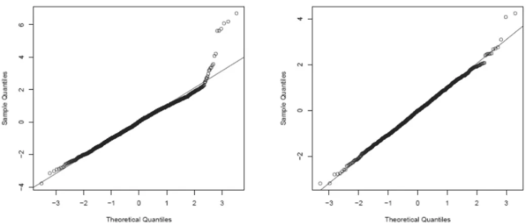
the linear components of the final model are reported in Table 4, Figure 2 depicts the non linear contributions to the linear predictors and Figure 3 depicts the ef-fects of relevant variables on E(Y), computed as explained in equation (10). Di-agnostics for the model (right panel of Figure 4) show a satisfactory fit. In par-ticular, the comparison of the normal probability plot of randomized residuals of the final model and that of residuals of the base model (left panel of Figure 4) clearly shows an improvement.
TABLE 4
Estimated coefficients (and their standard erros in parenthesis) for the linear components of the linear predictors of the Models 1 (ZIP), 2 (Poisson), 3 (Negative Binomial) ( denotes significance at 0.05, at 0.01, at 0.001)
Cathegories in the CF M1 M2 M3 -0.4052 -2.46625 -0.51 -0.22092 (Intercept) (-0.49576) (-0.70819) (-0.41868) (-0.59483) 0.01488 - 0.001425 -0.00143 age (-0.00436) - (-0.00376) (-0.00537) -0.20874 - -0.08275 -0.32228 gender=male (-0.18676) - (-0.13328) (-0.18067) 0.43405 - 0.644366 0.703936 d.cld (-0.15065) - (-0.18107) (-0.30186) 0.51566 - 0.272046 0.206823 d.exc.weight (-0.14901) - (-0.14614) (-0.21476) 0.48049 - 0.915369 1.07146 d.depress (-0.15409) - (-0.19388) (-0.29544) - -1.64512 0.313476 0.636713 d.cancer - (-0.70349) (-0.21001) (-0.32742) - -0.90944 -0.21804 -0.12977 d.emotional - (-0.41451) (-0.20985) (-0.31054) 2.76703 - 2.36435 2.183599 Physical characteristics race=native/other (-0.16296) - (-0.22758) (-0.51248) - 1.76584 -1.15078 -1.122182 Socioeconomic characteristics empl=employed - (-0.30828) (-0.12808) (-0.165605) -1.1606 -2.24915 -0.24561 0.008907 edu=college (-0.21879) (-0.48547) (-0.16456) (-0.206754) - 0.69069 -0.30207 -0.447153 Sociodemographic characteristics marstatus=neither - (-0.25804) (-0.11629) (-0.161664) -0.40496 - -0.37756 -0.380992 getalong=1 (-0.16232) - (-0.12954) (-0.18264) - 0.72674 -0.15234 -0.352367 sharevalues=1 - (-0.26977) (-0.11793) (-0.160707) 0.16901 0.39106 -0.08289 0.024304 neigh.satisf=2 (-0.19409) (-0.36479) (-0.14913) (-0.201376) 1.80436 2.08043 0.305088 0.309194 neigh.satisf=3 (-0.27243) (-0.79654) (-0.30372) (-0.437446) 0.05708 0.48203 -0.30419 -0.256483 neigh.satisf=4 (-0.26082) (-0.48789) (-0.20714) (-0.281482) 1.28446 1.0982 0.582118 0.570242 Neighbourhood neigh.satisf=5 (-0.25217) (-0.54051) (-0.21865) (-0.349067)
Figure 2 – Non linear contributions to the linear predictors for (BMI in panel (a) and income in panel (b)) and (age in panel (c)) of the final model (M1).
Figure 3 – Estimated conditional expectation of Y according to the final model (M1).
Figure 4 – Normal probability plot of randomized residuals for the base model M0 (left) and the final
4.2. Comparison with simpler models
In analysing count data as the number of hospitalization which is under con-sideration here the Poisson distribution is the most common modelling choice. When the Poisson model fails – as is easily seen to be the case here – alterna-tives include the Negative Binomial (NB) and the Zero Inflated Poisson (ZIP), whose appropriateness clearly depends on why the Poisson model actually fails. In particular, the ZIP is an explicit attempt at modelling an excess of zero counts: it, in fact, postulates that the counts come from one of two regimes: ei-ther a degenerate component with unit mass in zero or a Poisson distribution. Being in presence of an excess of zero counts which can be fruitfully modelled separately is a relatively common situation in medical and public health statistics (Lam et al., 2006). Such a model is also appealing on interpretation grounds since the probability of being in the zero-regime – which is explicitly estimated – may be interpreted as the probability of being in a lower risk group (subpopu-lation). (Clearly, this does not mean that one actually believes in the existence of two subpopulations.) The NB also allows for overdispersion with respect to a Poisson distribution but in a less specific way and does not share a similar in-terpretation.
It is worth noting that the ZIP distribution for Yi differs from a Poisson
distri-bution to the extent that i differs from 0 (since if i = 0 then Yi Poisson(i)).
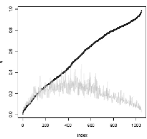
We may then get a hint about the relevance of the ZIP model by checking how often ˆi is significantly different from 0. We depict such a comparison in Figure 5 where we plot the estimates ˆi ordered increasingly and, as a reference, the value of the standard error of each ˆi multiplied by 1.96. Results show that ˆi is, in prevalence, different from 0. This graphical display substantially resembles the kind of tests which are commonly suggested in the literature (van den Broek, 1995; Rodrigues, 2006) where, usually, the hypotheses H0: = 0 is tested against
H1: 0 by means of a score test, whose main advantage is that one does not
need to estimate the more complicated Poisson model. Jansakul and Hinde (2002) consider a model in which i is modeled as a function of the covariate
(log[/(1-)] = X) and propose a score test for the hypotheses H0: = 0 versus
H1: 0. Rather than adapting the score test to the case of predictors with
smooth function we prefer estimating both model and compare them in Table 5. A test for ZIP versus Poisson can be based, since they are nested models, on the difference between the deviances (1484.8 - 1307 = 177.8) which, under M2, has a
Figure 5 – Sorted estimates ˆi (dots) in model M1, gray line is 0+1.96 s.e.(i).
In considering the ZIP as a model alternative to the Poisson (to be considered a basic model in this context) one should keep in mind, following El-Shaarawi (1985) but also Thas and Rayner (2005) that the mere preference for a ZIP over a Poisson model (that is, the fact that the lack of fit of the Poisson distribution is due to the excess of zeros) does not imply that the former is the appropriate choice, for this reason it is worth comparing the fit also against the NB.
In order to have a fair comparison of the ZIP, the Poisson (M2) and the NB
(M3) model, we estimate both M2 and M3 using as explanatory variables all
vari-ables included in the final model (in any linear predictor, in fact the conditional distribution of Y in the ZIP model depends on both and ). Estimates of coef-ficients are in Table 4.
BMI and income, whose contributions to the linear predictors in Figures 6 and 3 are similar in shape, play an analogous role in the three models (the linear pre-dictor in the Poisson and Negative Binomial models is directly related to E(Y ), so we can compare its shape with that of E(Y ) in the ZIP model). The contribu-tion of age is non significantly different than a constant in the models M2 and M3
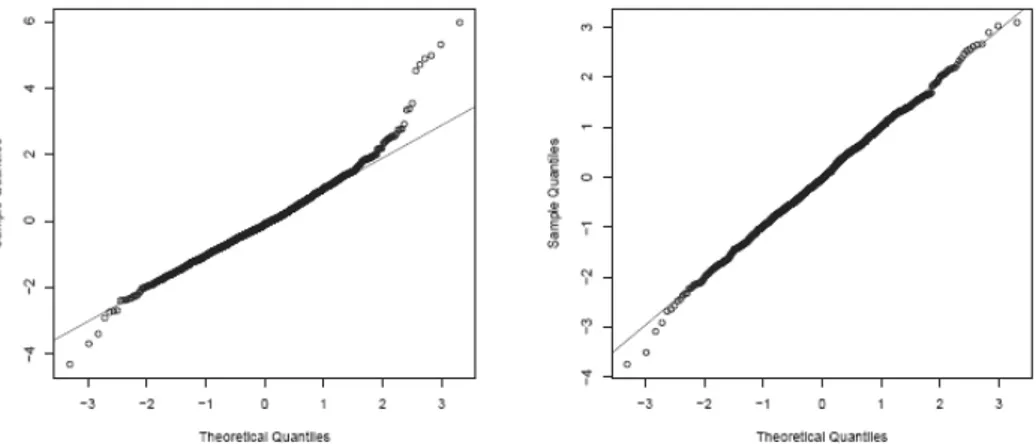
which may be the result of a lack of fit. The comparison of randomized residuals with a gaussian distribution (Figure 7) suggests lack of fit in the right tail for M2,
the Negative Binomial and ZIP models leading to a significant improve in that area (Figure 4). Moreover, we can compare their AIC and BIC values, such a comparison (Table 5) is in favour of the ZIP model, as already confirmed by the significance of the test previously discussed.
Thus, diagnostics and tests are consistently in favour of the more flexible Negative Binomial and ZIP models over the Poisson model, as intuition sug-gested beforehand. The comparison between the ZIP and NB models (based on the residuals in figures 4 and 7) leads to no clear cut conclusion.
TABLE 5
Comparison of ZIP, Poisson and Negative Binomial models: M1 is the final ZIP model; M2 and M3 are, respectively, the Poisson and Negative Binomial models involving all variables included in M1
d.f. AIC BIC deviance
M1 31 1368.99 1522.5 1307.0
M2 23 1530.76 1644.7 1484.8
M3 24 1370.99 1489.8 1323.0
Figure 6 – Contributions to the linear predictor for in the Poisson model M2 (top row) and in the
Negative Binomial model M3 (bottom row).
Figure 7 – Normal probability plot of randomized residuals for the Poisson model M2 (left) and the
5. FINAL REMARKS
Using data from the L.A.FAN Survey we have investigated whether some neighbourhood characteristics, measured by the perception of the individual, have a significant relationship with the expected number of hospitalizations (in two years). We have used generalized additive models which allow us to deal with non linear effects in a convenient way. This proved useful since the effects of BMI and income are clearly non linear. We also overcome to some extent the dif-ficulties in interpreting the results from a GAM with a ZIP distribution by simu-lating predicted values under varying assumptions in order to reveal the relation-ship of interest.
A comparison has been made between Poisson, Negative Binomial and ZIP models from which it emerged that the performance of the traditional Poisson distributional assumption for count data can be greatly improved. The results are not conclusive on whether a Negative Binomial or a ZIP model is to be pre-ferred, the latter, however is more flexible and so is preferred here. The choice of the model is relevant for our purposes since different models lead to different conclusions on the significance of the effect of the covariates (see Table 4).
It turns out relatively clearly that a high social cohesion leads to a lower hos-pitalization rate as shown by the fact that both the variables ‘getalong’ and ‘sharevalues’ have significant coefficients with signs implying in both cases a negative effect on the expected number of hospitalizations. Interestingly, the more general ‘satisfaction’ level concerning the neighbourhood does not show a clear effect.
Such results confirm the relationship of neighbourhood social environment on the health of individuals measured by the number of hospitalizations, particularly social cohesion which is, according to our results, more important than social control or public order. A strength of our evidences is that they do not depend on a specific definition of neighbourhood since each respondent refers (implic-itly) to his perception, on the other hand, this is also a limitation in that it does not allow to define ‘good’ and ‘bad’ neighbourhoods.
It is also worth saying that these results are coherent with those of Shin et al. (2006) in their fundamental conclusion even if the modelling framework is differ-ent.
Department of Statistical Sciences PIERANTONIO BELLINI
University of Padua
ISTAT DANIELA LO CASTRO
Department of Statistical Sciences FRANCESCO PAULI
REFERENCES
T. ABADA, F. HOU, B. RAM,(2007), Racially mixed neighborhoods, perceived neighborhood social cohesion,
and adolescent health in Canada, “Social science and medicine”, 65, 2004-2017.
P. BELLINI, D. LO CASTRO, F. PAULI,(2008),Perceived neighbourhood quality and adult health status:
new statistical advices useful to answer old questions?, “Technical Report 10-2008,
Diparti-mento di Scienze Statistiche, University of Padova”.
L. BERKMAN, I. KAWACHI, (2000), Social epidemiology, Oxford University Press.
D. BÖHNING, E. DIETZ, P. SCHLATTMANN, L. MENDONÇA, U. KIRCHNER, (1999), The zero-inflated
Poisson model and the decayed, missing and filled teeth index in dental epidemiology, “Journal of the Royal Statistical Society”, Series A 162, 195-209.
G. BOOTH, J. HUX,(2003),Relationship between avoidable hospitalizations for diabetes mellitus and
in-come level,“Archives of Internal Medicine”, 163, 101-106.
A. BOWLING, J. BARBER, R. MORRIS, S. EBRAHIM, (2006), Do perceptions of neighbourhood environment
influence health? Baseline findings from a British survey of aging, “Journal of Epidemiology and
Community Health”, 60, 476-483.
B. CHAIX, A. LEYLAND, C. SABEL, P. CHAUVIN, L. RSTAM, H. KRISTERSSON, J. MERLO, (2006), Spatial
clustering of mental disorders and associated characteristics of the neighbourhood context in Malmö, Sweden, in 2001. “Journal of Epidemiology and Community Health”, 60, 427-435.
B. CHAIX, J. MERLO, S. SUBRAMANIAN, J. LYNCH, P. CHAUVIN, (2005), Comparison of a spatial
perspec-tive with the multilevel analytical approach in neighborhood studies: The case of mental and behavioral disorders due to psychoactive substance use in Malmö, Sweden, 2001, “American Journal of
Epi-demiology”, 162, 171-182.
A. DIEZ ROUX, (2001), Investigating neighborhood and area effects on health, “American Journal of Public Health”, 91, 1783-1789.
A. EL-SHAARAWI, (1985), Some goodness-of-fit methods for the Poisson plus added zeros distribution, “Applied and environmental microbiology”, 49, 1304-1306.
A. ELLAWAY, S. MACINTYE, A. KEARNS,(2001), Perceptions of place and health in socially contrasting
neighbourhoods, “Urban Studies”, 38, 2299-2316.
R. FLOWERDEW, D. MANLEY, C. SABEL, (2008), Neighbourhood effects on health: does it matter where
you draw the boundaries?, “Social science and medicine”, 66, 1241-1255.
K. HUR, D. HEDEKER, W. HENDERSON, S. KHURI, J. DALEY, (2002), Modeling clustered count data with
excess zeros in health care outcomes research, “Health Services and Outcomes Research
Methodology”, 3, 5-20.
N. JANSAKUL, J. HINDE,(2002), Score tests for zero-inflated Poisson models, “Computational Statis-tics and Data Analysis”, 40, 75-96.
K. LAM, H. XUE, Y. CHEUNG,(2006), Semiparametric analysis of zero-inflated count data, “Biomet-rics”, 62, 996-1003.
A. LEE, K. WANG, J. SCOTT, K. YAU, G. MCLACHLAN, (2006), Multi-level zero inflated Poisson regression
modelling of correlated count data with excess zeros, “Statistical methods in medical research”,
15, 47-61.
Y. LI, Y. CHUANG, (2009), Neighborhood effects on an individual’s health using neighborhood
measure-ments developed by factor analysis and cluster analysis, “Journal of Urban Health”, 86, 5-18.
P. O’CAMPO,(2003), Invited commentary: Advancing theory and methods for multilevel models of
residen-tial neighborhoods and health, “American Journal of Epidemiology”, 157, 9-13.
R. PAMPALON, D. HAMEL, M. DE KONINCK, M. DISANT, (2007), Perception of place and health: differences
between neighbourhoods in the Québec City region, “Social science and medicine”, 65, 95-111.
C.E. PETERSON, N. SASTRY, A. R. PEBLEY, B. GHOSH-DASTIDAR, S. WILLIAMSON, S. LARA-CINISOMO, (2004), The Los Angeles Family and Neighborhood Survey, Codebook. RAND Corporation.
K. PICKETT, M. PEARL,(2001), Multilevel analyses of neighbourhood socioeconomic context and health
outcomes: a critical review. ”Journal of Epidemiology and Community Health”, 55, 111-122.
C. PROPPER, S. BURGESS, A. BOLSTER, G. LECKIE, K. JONES, R.J. JOHNSTON, (2007), The impact of
neighbourhood on the income and mental health of British social renters, “Urban Studies”, 44, 393-415.
R DEVELOPMENT CORE TEAM,(2005), R: A language and environment for statistical computing, Vi-enna, Austria: R Foundation for Statistical Computing. ISBN 3-900051-07-0.
F. RAJULTON, J. NIU, (2005), Health over the life course: A chain graph model of inter-relationships
among socio-demographic, societal and lifestyle factors, “XXV International Population Confer-ence”, International Union for the Scientific Study of Population (IUSSP), July 18-23, Tours, France.
R.A. RIGBY, D. STASINOPULOS, (2005), Generalized additive models for location, scale and shape, “Ap-plied Statistics”, 54, 507-554.
J. RODRIGUES,(2006), Full Bayesian significance test for zero-inflated distributions, “Communica-tions in Statistics - Theory and methods”, 35, 299-307.
N. SCHAEFER-MCDANIEL, (2009), Neighborhood stressors, perceived neighborhood quality, and child
mental health in New York City, “Health & Place”, 15, 148-155.
M. SHIN, W. CLARK, R. MAAS, (2006), Social capital, neighborhood perceptions and self-rated health:
Evi-dence from the Los Angeles Family and Neighborhood Survey (LAFANS), Working Paper CCPR-039-06, California Center for Population Research, UCLA.
S.E. SPIELMAN, E.H. YOO, (2009), The spatial dimensions of neighborhood effects, “Social Science and Medicine”, 68, 1098-1105.
D. STASINOPULOS, R. A. RIGBY, (2007), Generalized additive models for location scale and shape
(GAMLSS) in R, “Journal of Statistical Software”, 23, 1-46.
S. SUBRAMANIAN, D. KIM, I. KAWACHI, (2002), Social trust and self-rated health in US communities: a
multilevel analysis, “Journal of Urban Health”, 79, S21-S34.
C. TAYLOR, A. DAVID, M. WINKLEBY, (2006), Neighborhood and individual socioeconomic determinants
of hospitalization, “American Journal of Preventive Medicine”, 31, 127-134.
O. THAS, J. RAYNER, (2005), Smooth tests for the zero-inflated poisson distribution, “Biometrics”, 61, 808-815.
J. VAN DEN BROEK,(1995), A score test for zero inflation in a Poisson distribution, “Biometrics”, 51, 738-743.
M. WEDEN, R. CARPIANO, S. ROBERT, (2008), Subjective and objective neighborhood characteristics and
adult health, “Social science and medicine”, 66, 1256-1270.
M. WEN, C. R. BROWINING, A. C. KATHLEEN, (2007), Neighbourhood deprivation, social capital and
regular exercise during adulthood: a multilevel study in Chicago, “Urban Studies”, 44, 2651-2671.
M. WEN, L. HAWKLEY, J. CACIOPPO,(2006), Objective and perceived neighborhood environment,
individ-ual SES and psychosocial factors, and self-rated health: An analysis of older adults in Cook County, Illinois, “Social science and medicine”, 63, 2575-2590.
K. WILSON, S. ELLIOTT, M. LAW, J. EYLES, M. JERRETT, S. KELLER-OLAMAN, (2004), Linking perceptions
of neighbourhood to health in Hamilton, Canada, “Journal of Epidemiology and Community Health”, 58, 192-198.
SUMMARY
Modeling the relationship between perceived neighbourhood characteristics and adult hospitalization fre-quencies from a cross-sectional study
Interest in the quantitative effects of neighbourhood characteristics on urban health has recently increased in social epidemiology. Such effects are mostly studied employing multilevel models based on some definition of the neighbourhood. We investigate the sta-tistical relationship between health and the neighourhood quality as perceived by indi-viduals, thus avoiding the need of choosing a specific definition of neighbourhood.
We use data from the Los Angeles Family and Neighbourhood Survey (L.A.FANS). We measure health status of an individual as the number of hospitalizations in the last two years. This number is related to individual carachteristics (including neighbourhood perceptions) through generalized additive models (GAM), focusing particularly on the Zero Inflated Poisson (ZIP), which is an unusual choice in this context.
We also overcome to some extent the difficulties in interpreting the results from a GAM with a ZIP distribution by simulating predicted values under varying assumptions in order to reveal the relationship of interest.
The analysis confirms that the quality of neighbourhood – as measured by perceptions of individuals – significantly relates to the health status of inhabitants – as measured by the number of hospitalizations.