Published by Canadian Center of Science and Education
Size and Value Anomalies in European Bank Stocks
Barbara Fidanza1 & Ottorino Morresi2 1 Department of Law, University of Macerata, Italy
2 Department of Economics, Roma Tre University, Italy
Correspondence: Barbara Fidanza, Department of Law, University of Macerata, Italy. E-mail: [email protected]
Received: February 12, 2018 Accepted: October 17, 2018 Online Published: November 20, 2018 doi:10.5539/ijbm.v13n12p227 URL: https://doi.org/10.5539/ijbm.v13n12p227
Abstract
The Fama-French three-factor model (Fama & French, 1993) has been subject to extensive testing on samples of US and European nonfinancial firms over several time windows. The most accepted evidence is that size premium (SMB) and value premium (HML) other than the market risk premium help explain cross-section and time-series changes in stock returns. However, scholars have always paid little attention to the financial industry because of the intrinsic differences between financial and nonfinancial firms. The few studies that tested the model on financial firms found mixed evidence on the role of size and book-to-market ratio (B/M) in explaining stock returns. This paper tries to bridge the gap by testing the model on a sample of European financial firms. We find that size and B/M factors seem to be sources of undiversifiable risks and should therefore be included as risk premiums for estimating expected returns of financial firms. Small and high-B/M firms show higher returns that are not explained by market risk and the inclusion of SMB and HML helps improve the regression models’ goodness-of-fit.
Keywords: equity returns, stock returns, three-factor model, pricing model 1. Introduction
Pricing models are charged with the task to identify factors explaining the return of risky assets. They are employed in many theoretical and operational finance areas such as event study to test capital market efficiency and the value effects of corporate finance choices (e.g., capital structure decisions, dividend policy, M&A announcements, etc.), management and performance evaluation of funds and portfolios, cost of capital estimation in capital budgeting issues, and so on.
The theory of capital market equilibrium faces the problem by identifying the appropriate relationship between a risk measure and the expected return. The first formalized theory of market equilibrium can be identified in the Capital Asset Pricing Model (CAPM) independently developed by Treynor (1962), Sharpe (1964), Lintner (1965), and Mossin (1966) (hereafter, SL model). The validity of the risk-return relationship proposed by the SL model was further tested by several empirical studies (e.g., Black et al., 1972; Fama and MacBeth, 1973; Gibbons, 1982; Stambaugh, 1982) that largely found inconsistent results with the CAPM basic assumptions.
Empirical tests often failed to support the SL model mainly because of the following reasons. First, methodological issues may affect test results. Empirical tests rely on two widely recognized methodologies: times-series regressions, where monthly or weekly portfolio excess returns are regressed on monthly or weekly market excess returns, and cross-section regressions, where average portfolio excess returns are regressed on portfolio betas estimated by first-pass times-series regressions. Cross-section tests may therefore be affected by errors in beta estimation. Some scholars (e.g., Miller and Scholes, 1972; Roll, 1977) someway tried to correct beta estimations, some other (Beaver et al., 1970) attempted to estimate the true beta directly by means of corporate fundamentals which it is based on (instrumental beta).
Second, CAPM assumptions may be to a certain extent unrealistic. Inconsistent results may be due to frictions and market imperfections such as taxes, non-homogeneous expectations, different lending and borrowing rates, etc., the CAPM does not incorporate (Brennan, 1970; Black, 1972; Mayers, 1972; Lindenberg, 1979; Mayshar, 1981). Third, market beta may not be sufficient to explain cross-sectional changes in stock returns as investors need to be rewarded for additional, non-diversifiable risk factors. This means that market portfolio is inefficient and market
risk is not the unique source of risk. This explanation brought to the existence of the so called multifactor pricing models which take into account multiple causes of risk. The first formalized multifactor model was the Arbitrage Pricing Theory (Ross, 1976) which may include further risk factors such as macroeconomic and financial variables other than the market index. Multifactor models may also take into account corporate fundamentals such as market capitalization (MV), price-to-earnings ratio (P/E), price-to-cash flow per share ratio (P/CF), book-to-market ratio (B/M), etc., provided that they are linked to risk sources which investors require a compensation for. Fama-French three-factor model (TFM) (Fama and French, 1993) is probably the most studied and popular multifactor model. It shows that risk premiums built on market capitalization (MV) and book-to-market ratio (B/M) are significantly correlated with stock excess returns of non-financial firms and, combined with the market risk premium, significantly improve the model explanatory power.
This work belongs to the third body of literature and aims at verifying whether the TFM may fit to explain changes in stock returns of a sample of financial firms listed on European stock markets. The analysis is motivated by the following reasons:
a) the topic is highly debated internationally and this is confirmed by the number and relevance of studies that focus on it;
b) financial firms are strongly neglected by empirical studies as they are considered intrinsically different from industrial firms. The risk exposure of banks and its relation with stock returns is estimated by means of different approaches and takes into account specific risk factors such as interest rate risk, credit risk, real-estate risk, exchange rate risk, etc.;
c) understanding bank risk factors is becoming increasingly important as a result of deregulation, the recent financial crisis, Basel rules on capital requirements, leverage ratio, and liquidity requirements that emphasize more and more market risk factors.
The paper is organized as follows: section two summarizes the main empirical evidence; section three describes sample and methodology; section four illustrates and discusses results; section five concludes.
2. Literature Review
According to several scholars, a significant relationship between some fundamental variables and stock returns may arise, as the SL model cannot price some risk sources. Market beta could therefore have little information about the cross-section of average returns. If stocks are rationally priced, their returns should reward the sensitivity to the variation of these variables.
Fama and French (1993) model a risk-return relationship in which two fundamental variables such as firm size (market capitalization) and B/M are added to the market risk premium. The same authors, in another essay (Fama and French, 1992), demonstrate that these two variables help explain the cross-section of stock returns and are therefore risk factors that the SL model does not consider.
In their equilibrium model (hereafter, TFM), the risk premium of the i-th asset is defined as follows:
(
)
i f i m f i i
R
−
R
=
β
R
−
R
+
s SMB h HML
+
The first risk component (
β
i) is the sensitivity to the market risk as defined in the SL model; the second risk component (s
i) is the sensitivity to the risk factor related to firm size (i.e., size premium: small firms are riskier than large firms); the third risk component (h
i) is the sensitivity to the risk factor related to the B/M (i.e., value premium: firms with high B/M values are riskier than firms with low B/M values). SMB (small-minus-big) and HML (high-minus-low) are risk premiums that express the extra-return for one unit of risk, respectively,s
i andi
h
;(
Rm−Rf)
is the risk premium for one unit of market risk (β
i).Size and B/M should proxy for default risk and uncertainties about growth prospects and future profitability. Small firms are likely to be more exposed to bankruptcy and high-B/M firms should perform poorly relative to low-B/M firms.
TFM has internationally been tested largely on samples of non-financial listed firms. Arshanapalli et al. (1998) test TFM in 18 stock markets, of which 10 are Europe-based, from 1975 to 1995. Their results suggest that TFM does not work in the US stock exchanges, but in other markets size and B/M risk factors are relevant in explaining stock returns. Griffin (2002) shows that TFM performs better if risk factors are defined domestically rather than internationally including the US, Canada, Japan, and the UK. Moerman (2005), on a sample of stocks coming from 11 countries and investigated from 1991 to 2001, points out that TFM seems to work well in the European stock markets and confirms, according to Griffin (2002), that the Fama-French risk factors are country-specific.
Al-Mwalla and Karasneh (2011) find that size and B/M factors help explain variations in stock returns also in emerging markets.
Other works (Kothari et al., 1995; Daniel and Titman, 1997; Davis et al., 2000; Taneja, 2010; Manjunatha and Mallikarjunappa, 2011; Eraslan, 2013; Foye et al., 2013; Sehgal and Balakrishnan, 2013; Sharma and Mehta, 2013) show that:
- excess returns are well enough explained by the SL model; market beta is always positive and R2 often
exceeds 60%;
- SMB and HML alone are significantly related to excess returns but the explanatory power of the model without the market risk premium is significantly lower;
- the model showing the best fitting is that including all three risk premiums. In the above studies, except Daniel and Titman (1997), R2 is greater than 90% in a good number of cases.
With reference to non-US companies, Fama and French (2012) show that there is a negative but not statistically significant size premium in Europe, Japan, and Asia-Pacific and a significant value premium in all regions (North America, Asia-Pacific, Europe, Japan).
Chaudhary (2017) finds that although CAPM can capture the cross section variability of returns both in India and US, the three factor model with size and value factors still work better and hence is useful in pricing the financial assets of both developed and developing countries. In the Indian stock market in the period from April 1, 2009 to March 31, 2016, the three-factor model failed to capture the variability of asset returns, but it explains the portfolio asset returns sorted by size and value (Anwar and Kumar, 2018).
The most recent developments of literature assert that a five-factor model including market risk premium, size, value, profitability, and investment patterns, performs better than the tree-factor model (Fama and French, 2015). Specifically, the profitability factor and investment factor, when the link is positive, capture the high average returns associated with low market beta, share repurchases, and low stock return volatility (Fama and French, 2016). Conversely, a negative effect of the two factors, like those of relatively unprofitable firms that invest aggressively, helps explain the low average stock returns associated with high beta, large share issues, and highly volatile returns.
A cross-country test highlighted that the effects of five factors are different in different regions. The average stock returns in North America, Europe, and Asia Pacific increase with the book-to-market ratio (B/M) and profitability and are negatively related to investment. In Japan, the relation between average returns and B/M is strong, but average returns are poorly related to profitability or investment (Fama and French, 2017).
Focusing on the financial industry, for years interest rate was thought to be the most important variable to be added to the market risk premium in the SL model. Giliberto (1985) however shows that studies taking into account interest rate as common risk factor are not reliable as a result of biases in OLS estimates due to problems in orthogonalization. Following studies have used different approaches to measure the sensitivity of bank stock returns to variables other than the market risk premium such as interest rate risk, credit risk, real-estate risk, exchange rate risk, etc. (Lynge and Zumwalt, 1980; Flannery and James, 1984; Kane and Unal, 1988; Choi et al., 1992; Bessler and Booth, 1994; Allen et al., 1995; Mei and Saunders, 1995; Choi and Elyasiani, 1997; Chamberlain et al., 1997; Demsetz and Strahan, 1997; Hess and Laisathit, 1997; Dewenter and Hess, 1998; Oertmann et al., 2000; Bessler and Murtagh, 2004; Martins et al., 2012; Gounopoulos et al., 2013). They conclude that even if these additional factors somehow matter, being related to the traditional operations of financial intermediaries, they do not allow us to build a multifactor equilibrium model able to reward banks’ non-diversifiable risk factors.
TFM finds little application in banking. The main reason is that bank leverage is intrinsically very high and, according to Modigliani and Miller (1958 and 1963), financial risk caused by high debt ratios should be incorporated in equity beta. Moreover, bank size and B/M are not likely to proxies for the same risk sources as for industrial firms. However, Modigliani-Miller propositions do not reject CAPM assumptions therefore restricting empirical tests of CAPM and TFM to non-financial firms is to some extent arbitrary.
Barber and Lyon (1997) show that B/M and size risk factors tend to explain stock returns of financial firms listed on the NYSE from 1973 to 1994 in a similar way as for non-financial ones. Schuermann and Stiroh (2006) compare several pricing models on a sample of bank stocks observed from 1997 to 2005 and conclude that market, B/M, and size risk factors are the most important in explaining changes in stock returns. Viale et al. (2009) test CAPM, TFM, and ICAPM (intertemporal capital asset pricing model) on a sample of US financial firms over the period 1986-2003 and conclude that (1) ICAPM is the most effective, (2) TFM does not help improve significantly
CAPM, and (3) the value premium is a better predictor than the size premium. Baek and Bilson (2015), on a sample of financial and non-financial US firms analyzed from 1963 to 2012, document that TFM works worse if applied to financial firms but may anyway be used to price adequately bank stocks.
Drobetz et al. (2007) investigate the impact of individual bank fundamental variables on stock returns using data from a panel of 235 European banks from 1991 to 2005. Their results indicate that several bank-specific variables exhibit a robust explanatory power across different model specifications: there is a positive impact of the ratio of loans to total assets, the ratio of non-interest income to total income, and the ratio of off-balance sheet items to total assets on subsequent bank stock returns.
Bessler et al. (2014) study the time-varying risk exposures of US bank holding companies for the 1986 to 2012 period by decomposing total bank risk into systematic banking-industry risk, systematic market-wide risk, and idiosyncratic bank risk. Their results suggest that corporate credit risk and real estate risk are more detrimental during crises, while banks’ interest rate risk sensitivity has changed over the last decade. The banks’ equity ratio, loan-loss provisions, fraction of real estate loans, and proportion of non-interest income relate to the differences in individual bank risk. Moreover, banks’ idiosyncratic risk contains a strong state-level business cycle component. Their results are robust to alternative risk factor specifications.
3. Sample and Methodology
The sample investigated is composed of financial stocks that, on 30 June of each year from 2002 to 2011, are listed on the main European stock exchanges (Austria, Belgium, Denmark, Finland, France, Germany, Greece, Ireland, Italy, Norway, Poland, Portugal, Spain, Sweden, Switzerland, UK). Variables used in the analysis are collected yearly on June in order to make accounting data available. We use monthly returns and require a stock to be listed for at least 24 months in order to have a sufficient number of monthly observations needed to construct portfolios sorted by pre-ranking beta. Only stocks with complete data are included. All variables are collected from Datastream - Thomson Reuters. The size of the final sample changes over time and goes from 138 to 171 stocks (Table 1). Table 1. Sample Year Country 2002 2003 2004 2005 2006 2007 2008 2009 2010 2011 Austria 6 6 6 6 6 7 6 7 7 7 Belgium 2 2 3 3 3 3 3 3 3 3 Denmark 22 23 23 23 23 23 24 25 25 25 Finland 2 2 2 2 2 2 2 2 2 3 France 13 14 17 17 16 18 18 20 20 20 Germany 6 6 6 6 8 8 9 9 9 9 Greece 7 7 7 7 7 8 8 8 8 8 Ireland 2 2 2 2 2 2 2 2 2 2 Italy 17 17 18 19 19 19 19 19 18 19 Norway 17 17 17 17 17 20 20 22 22 22 Poland 9 10 10 11 12 12 12 12 12 12 Portugal 3 3 3 3 3 3 3 3 2 3 UK 4 4 4 4 4 4 5 5 5 6 Spain 4 5 5 5 5 5 5 6 6 6 Sweden 4 4 4 4 4 4 4 4 4 4 Switzerland 20 21 21 21 20 22 22 22 22 22 Total 138 143 148 150 151 160 162 169 167 171
The table shows the number of stocks included in the sample by country and year. Empirical analysis is based on two steps:
- first of all, we perform a descriptive analysis in order to verify whether there is a cross-sectional link between stock returns and potential common risk factors;
- second, at portfolio level, we perform time-series regressions in order to test the TFM. We report below some details of the methodology followed.
3.1 Descriptive Analysis
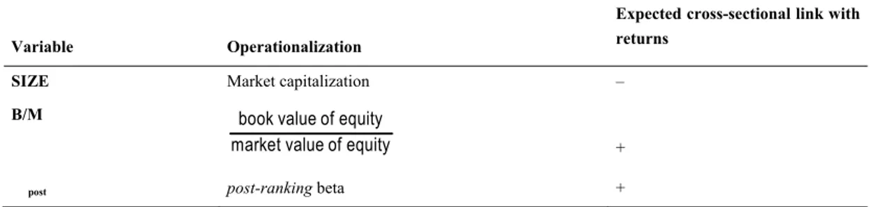
This analysis aims at identifying causality relationships between returns and potential explanatory variables in a pricing model. For each stock and for each year we detect the value of variables that could proxy for risk factors. Next we build several portfolios sorted by each variable and calculate the times-series mean of portfolio returns over the entire observation period in order to uncover whether changes in that variable affect portfolio returns. Table 2 describes the main variables used in the analysis.
Table 2. Proxy variables
Variable Operationalization
Expected cross-sectional link with returns
SIZE Market capitalization –
B/M book value of equity
market value of equity +
post post-ranking beta +
The table shows variables, their operationalization, and the projected relationship with returns. Post-ranking beta
Following Fama and MacBeth (1973), on 30 June of each year, sampled stocks are sorted in ascending order by SIZE and pre-ranking beta. Pre-ranking beta is estimated by regressing monthly stock returns on the Datastream Market Index over a 2-year time period. This beta is calculated before the sorting date as opposed to the post-ranking beta that is estimated after the sorting date.
By means of this double sorting we have 25 portfolios updated yearly: 5 portfolios sorted by SIZE (SIZE-1, SIZE-2, SIZE-3, SIZE-4, SIZE-5); each of them, in turn, is sorted in further 5 portfolios by pre-ranking beta (BETA-1, BETA-2, BETA-3, BETA-4, BETA-5). Each portfolio therefore contains 4% of all stocks included in the sample for that year. For example, portfolio 1 includes the smallest firms and those with the smallest pre-ranking beta, portfolio 5 includes the smallest stocks but with the largest pre-ranking beta, and so on. Every Tth year, for each stock, we estimate monthly returns for the subsequent 12 months, that is, returns from 31 July of year T to 30 June of year T+1. We therefore have 18,708 monthly returns (i.e., 12 monthly returns times 1,559 stock-year observations from 2002 to 2011). Returns for security i in month t
( )
Rit and market returns in month t( )
Rmt are defined as the relative change, respectively, of the official price adjusted for equity issues, stock splits, and dividends, and of the price index calculated by Datastream.For every t th month that follows 30 June of Tth year we calculate the monthly average return (i.e., portfolio return) for each of 25 portfolios. We therefore obtain a series of 120 monthly returns (from July 2002 to June 2012) used to estimate the post-ranking beta (βp) for the pth portfolio. We assign the same post-ranking beta to the same-portfolio stocks. This means that a security may change its beta if it switches portfolio over time.
This methodology is commonly used for two main reasons:
- first, size and beta of stocks are demonstrated to be highly correlated. This makes it undesirable to calculate single-stock beta but rather beta of portfolios composed of similar stocks in terms of beta and size so as to shade the beta-size relationship. Second, it is well known that beta estimation for single stocks may suffer autocorrelation of residuals that leads to underestimation of the variance of regression coefficients thereby increasing the value of Student t. This makes test statistics unreliable and increases the likelihood to reject the null hypothesis that the coefficient is equal to zero. Portfolio beta estimates are less affected by this problem;
- portfolio post-ranking beta is estimated by using the entire series of returns over the period under investigation. This approach may be attacked as it assumes beta to be stable over time. However, Chan and Chen (1988) demonstrate that over long time horizons post-ranking beta at portfolio level is more accurate and stable as a result of the stationarity of the time series distribution of betas. This assures that the error we make by assigning
the time series average of betas (
β
p) to the portfolio p is proportional to the difference betweenβ
p and the cross-sectional mean of average betas( )
β
. The following relation therefore holds:(
)
pt p
K
pβ
−
β
=
β
−
β
K is a zero-mean constant and does not depend on portfolio characteristics but market trend: it takes negative values during market growth and positive values during market downturns.
The relationship between returns and post-ranking beta is supposed to be positive according to the CAPM. This relationship is not always confirmed by empirical studies that sometimes find not statistically significant coefficients.
Size
The relationship between size and returns, known as size effect, is generally found to be negative (e.g., Banz, 1981). This means that small firms earn greater risk-adjusted returns than large firms. However, later studies, that take into account the post-eighties period, also find that larger firms perform better than small firms in some sub-periods (e.g., Dimson & Marsh, 1999; Horowitz et al., 1999 and 2000; Chan et al., 2000).
This effect could just be due to the influence of size on equity beta. Yet, sorting stocks by beta and size, the empirical evidence often finds larger returns to small stocks without showing any clear link between size and beta. Possible explanation is that small firms face higher information asymmetry, uncertainties about future profits, and distress costs. The result is that investors are expected to be rewarded with higher returns.
Some scholars (e.g., Berk, 1995) criticize the use of market capitalization as proxy for the firm size. Market capitalization depends on a firm’s cash flows and cost of capital. Large firms are likely to produce more cash flows but this does not assure a higher market value to the extent that the cost of capital is high as well. However, alternative measures of firm size such as book value of total assets, book value of tangible assets, sales, number of employees, etc., seem to result in the same relationship.
Book-to-market ratio (B/M)
Book-to-market ratio (B/M) is strongly and positively related to stock returns in all studies. What it tells us about a firm’s risk is not always clear as many firm characteristics may be reflected by this ratio. Low-B/M firms are generally known as glamour stocks and supposed to show higher-than-mean growth rates, better growth opportunities, and a lower risk than high-B/M firms, known as value stocks.
Agency theory may also help explain the higher risk of value firms. When growth options are poor, managers may use available cash with more discretion thereby increasing the probability of undertaking bad projects, the risk equity holders bear, and the return they expect.
3.2 Time-Series Regressions
On 30 June of every year stocks are sorted in ascending order by SIZE and B/M so as to create 25 portfolios SIZE-B/M. For each portfolio p at month t we estimate monthly returns (Rpt) over 12 months that follow the
sorting date thereby obtaining 25 series composed of 120 monthly average returns (i.e., 10 years times 12 months). Regression analysis involves each portfolio according to 3 different models: (1) portfolio excess returns (Rpt −Rft) are regressed on market risk premium
(
R
mt−
R
ft)
; (2) portfolio excess returns (Rpt−Rft) are regressed on size premium (SMB
t) and value premium (HML
t); (3) portfolio excess returns (Rpt −Rft) areregressed on all three premiums. Time-series regressions allow us to estimate (a) how much the portfolio returns are sensitive to changes of various risk premiums over time, (b) the ability of each model to predict portfolio returns accurately, that is, the share of the portfolio return variability explained by variation in risk premiums. Variables used in the regression analysis are operationalized as follows:
f
(
Rm−Rf)
: the market risk premium is the difference between Datastream Market Index and the risk-free rate.In order to estimate SMB and HML, we sort stocks by SIZE and B/M and obtain 6 portfolios: 2 portfolios sorted by size (B = big portfolio and S = small portfolio) and 3 portfolios sorted by B/M (L = low-B/M portfolio; M = medium-B/M portfolio; H = high-B/M portfolio).
SMB (small-minus-big): difference between the average return of three small portfolios and the average return of three big portfolios ( / ) ( / ) ( / ) ( / ) ( / ) ( / )
3 3 S L + S M + S H B L + B M + B H − .
HML (high-minus-low): difference between the average return of two high-B/M portfolios and the average return of two low-B/M portfolios ( / ) ( / ) ( / ) ( / )
2 2
S H + B H S L + B L
−
.
SMB and HML estimation procedure aims at removing the potential dependence between size and B/M. The reliability of this technique is demonstrated by a very low correlation coefficient between SMB and HML (i.e., 0.0007, Table 3, panel A).
Table 3. Dependent and independent variables
Panel A: correlation matrix
(
Rm−Rf)
SMB HML(Rm −Rf) 1.0000
SMB 0.1555 1.0000
HML 0.2990 0.0007 1.0000
Panel B: descriptive statistics
Independent variables Monthly average returns Std. Deviation
(
Rm−Rf)
0.0204 0.0641SMB 0.0018 0.0512
HML 0.0052 0.0369
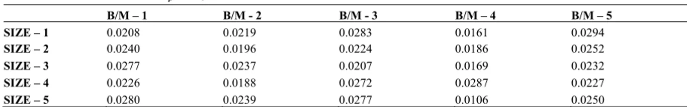
Panel C: dependent variable Rp −Rf (monthly average returns)
B/M – 1 B/M - 2 B/M - 3 B/M – 4 B/M – 5 SIZE – 1 0.0208 0.0219 0.0283 0.0161 0.0294 SIZE – 2 0.0240 0.0196 0.0224 0.0186 0.0252 SIZE – 3 0.0277 0.0237 0.0207 0.0169 0.0232 SIZE – 4 0.0226 0.0188 0.0272 0.0287 0.0227 SIZE – 5 0.0280 0.0239 0.0277 0.0106 0.0250
Panel A shows Pearson correlations between independent variables; Panel B shows mean and standard deviation of independent variables; Panel C shows monthly average returns of 25 portfolios sorted by size and book-to-market ratio (B/M).
Three regression models may be summarized as follows: (1)
R
pt−
R
ft=
α
p+
β
p(
R
mt−
R
ft)
+
ε
pt(2)
R
pt−
R
ft=
α
p+
s SMB
p t+
g HML
p t+
ε
pt(3)
R
pt−
R
ft=
α
p+
β
p(
R
mt−
R
ft)
+
s SMB
p t+
g HML
p t+
ε
pt withp
=1,2
andt
=1,2
.(Rpt −Rft),
(
Rmt −Rft)
, SMBt and HMLt are therefore vectors of 120 monthly returns.β
p,s
p andg
p areregression coefficients expressing the sensitivity of portfolio risk premiums to time-series changes of, respectively, market risk premium, size premium, and value premium.
4. Results
4.1 Descriptive Analysis
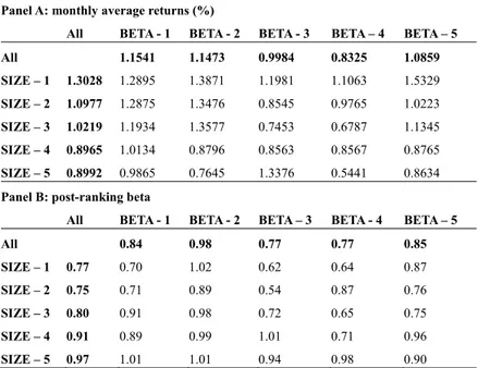
Table 4. Monthly average returns and post-ranking beta for 25 SIZE-BETA portfolios
Panel A: monthly average returns (%)
All BETA - 1 BETA - 2 BETA - 3 BETA – 4 BETA – 5 All 1.1541 1.1473 0.9984 0.8325 1.0859 SIZE – 1 1.3028 1.2895 1.3871 1.1981 1.1063 1.5329 SIZE – 2 1.0977 1.2875 1.3476 0.8545 0.9765 1.0223 SIZE – 3 1.0219 1.1934 1.3577 0.7453 0.6787 1.1345 SIZE – 4 0.8965 1.0134 0.8796 0.8563 0.8567 0.8765 SIZE – 5 0.8992 0.9865 0.7645 1.3376 0.5441 0.8634
Panel B: post-ranking beta
All BETA - 1 BETA - 2 BETA – 3 BETA - 4 BETA – 5 All 0.84 0.98 0.77 0.77 0.85 SIZE – 1 0.77 0.70 1.02 0.62 0.64 0.87 SIZE – 2 0.75 0.71 0.89 0.54 0.87 0.76 SIZE – 3 0.80 0.91 0.98 0.72 0.65 0.75 SIZE – 4 0.91 0.89 0.99 1.01 0.71 0.96 SIZE – 5 0.97 1.01 1.01 0.94 0.98 0.90
Panel A shows monthly average returns of 25 portfolios sorted by size and pre-ranking beta; Panel B shows post-ranking beta of 25 portfolios sorted by pre-ranking beta and size.
Table 4 shows, for each portfolio sorted by size and pre-ranking beta, average monthly returns (Panel A) and portfolio post-ranking beta (Panel B). Table 4 allows us to outline some relationship between returns, size, and beta. Sorting stocks by size only (first column, Panel A), the smallest portfolio (SIZE - 1) earns a monthly return equal to 1.3028% compared to the largest portfolio that earns 0.8992% on average. In general, small stocks seem to produce higher average returns than large stocks and this trend appears to hold also for each portfolio sorted by pre-ranking beta. However, moving from large to small stocks, while returns go up, post-ranking beta does not (first column, Panel B) and this is not consistent with the SL model. Another relevant point is that a beta change (first row, Panel B) does not always go together with a same-type change of returns (first row, Panel A).
Table 5. Monthly average returns (%) of portfolios sorted by fundamental variables
Panel A: monthly average returns (%) of portfolios sorted by fundamental variables Portfolios 1 2 3 4 5 Orderi ng variable Pre-ranking beta 1.154 1.147 0.998 0.832 1.085 SIZE 1.302 1.097 1.021 0.896 0.899 B/M 0.288 0.289 0.317 0.753 0.656
Panel B: returns and post-ranking beta of portfolios sorted by size and B/M
SIZE – 1 SIZE – 2 SIZE – 3 SIZE – 4 SIZE – 5 Returns (%) 1.302 1.097 1.021 0.896 0.899
Post-ranking beta 0.772 0.754 0.802 0.912 0.968
B/M – 1 B/M – 2 B/M – 3 B/M – 4 B/M – 5 Returns (%) 0.288 0.289 0.317 0.753 0.656
Panel A reports monthly average returns of portfolios sorted by each of the fundamental variables (pre-ranking beta, size, and B/M). Panel B reports returns and post-ranking beta of portfolios sorted by size and B/M.
On June of each year, stocks are sorted in ascending order by each of the variables shown in Table 2 so as to form 5 portfolios whose monthly average returns are then estimated over a 120-month period (Table 5). Panel A of Table 5 shows these returns. Panel B of Table 5 reports monthly average returns and post-ranking beta of portfolios sorted by size and B/M.
The results show that high-B/M portfolios yield higher returns: Panel A shows that moving from portfolio 1 (B/M - 1) to portfolio 5 (B/M - 5), returns steadily increase from 0.288% to 0.656%. Size confirms the evidence already shown, that is, small firm portfolios earn greater returns than large firm portfolios.
In the same way as for size, high-B/M portfolios are not associated with higher post-ranking beta. This means that higher returns earned by high-B/M portfolios do not seem to be explained by higher betas.
In summary, at this level of analysis, financial firms seem to behave like industrial firms in terms of risk factors: size and B/M appear to be linked to stock returns with small and high-B/M firms performing better than large and low-B/M firms. These relations do not seem to be explained by market beta and would support the implementation of a multifactor model of risk in which size premium and value premium are added to the market risk premium. 4.2 Results of Time-Series Regressions
Tables 6, 7, and 8 show results of time-series regressions run on each of three models, respectively, SL model, model with size premium and value premium alone, three-factor model. Each row corresponds to the respective portfolio which the regression is performed on. Columns of the tables report, for each regression, regression coefficients
α
p,β
p, sp, gp, adjusted R-squared, and F-test significance level. Regressions between portfolio risk premium and market risk premium Table 6 reports the following main results:
- Intercept is always statistically different from zero (except regression 18). This is not consistent with the SL model.
- Slope (
β
p) is always positive and significantly different from zero. Market risk premium is therefore strongly linked to the risk premium of each portfolio according to the SL model. Market beta goes from a minimum of 0.4042 (portfolio 14) to a maximum of 1.4124 (portfolio 24). The bigger the firms in the portfolio, the larger the market beta seems to be therefore showing that returns of large firms appear to be more sensitive to market risk. However, this result should be taken with caution because of the intervalling-effect bias in beta estimates. The sensitivity of a stock’s excess returns to the market excess returns is influenced by the length (e.g., daily, weekly, monthly, etc.) of the return interval used in estimating betas. Indeed, stock prices respond to new information more or less quickly depending on stock liquidity that, in turn, is affected by firm size. Small caps are less known, infrequently traded, and therefore adjust with delay, while large caps are better known, traded, and their price changes faster. As a consequence, for large firms, the smaller the length of the return interval, the higher the sensitivity of stock prices to market movements tends to be. Undersized return interval may therefore cause betas to be overestimated. While small caps show an opposite trend: betas tend to be overestimated when the return interval is oversized (e.g., Cohen et al., 1983; Jones and Yeoman, 2012; Hong and Satchell, 2014).- F-test always shows a high level of significance while the model goodness-of-fit is not always good: adjusted R-squared is higher than 50% in 6 portfolios and in 3 of them exceeds 60%. In the remainder of them it is almost always lower than 30% and shows the need to find additional risk factors other than the market risk.
- Larger R-squared (i.e., greater than 50%) are found in portfolios with large firms (SIZE-4 and SIZE-5). This points out that portfolio return variability explained by market risk premium is bigger in large-sized firms.
Table 6. Time-series regressions: returns and market risk premium αp
β
p Adj. R2 sign(F) 1 SIZE – 1 B/M – 1 *0.0041 *0.5895 0.3300 0.000 2 B/M – 2 *0.0146 *0.4045 0.2359 0.010 3 B/M – 3 *0.0174 *0.5307 0.3958 0.012 4 B/M – 4 *0.0041 *0.5895 0.3380 0.003 5 B/M – 5 *0.0155 *0.4351 0.3314 0.004 6 SIZE – 2 B/M – 1 *0.0101 *0.4148 0.3054 0.000 7 B/M – 2 *0.0044 *0.7417 0.3005 0.000 8 B/M – 3 *0.0118 *0.5193 0.4210 0.006 9 B/M – 4 *0.0101 *0.4148 0.3054 0.008 10 B/M – 5 *0.0150 *0.5019 0.3992 0.000 11 SIZE – 3 B/M – 1 *0.0136 *0.6902 0.4477 0.002 12 B/M – 2 *0.0034 *0.9916 0.3959 0.001 13 B/M - 3 *0.0035 *0.8449 0.3665 0.000 14 B/M - 4 *0.0086 *0.4042 0.2284 0.008 15 B/M - 5 *0.0130 *0.4980 0.2012 0.000 16 SIZE – 4 B/M - 1 *0.0005 *1.0841 0.6684 0.005 17 B/M - 2 *0.0051 *0.6708 0.5149 0.011 18 B/M - 3 0.0096 *0.8614 0.6247 0.000 19 B/M - 4 *0.0096 *0.9319 0.4766 0.000 20 B/M - 5 *0.0057 *0.9445 0.4239 0.006 21 SIZE – 5 B/M - 1 *0.0086 *0.9525 0.5882 0.000 22 B/M - 2 *0.0023 *1.0559 0.6907 0.000 23 B/M - 3 *0.0070 *1.0148 0.5266 0.000 24 B/M - 4 *0.0149 *1.4124 0.2887 0.000 25 B/M - 5 *0.0096 *0.9251 0.3433 0.000 * Statistically significant at the 1% levelTable 6 reports the results of the regression model in which returns of each portfolio are regressed on market risk premium.
α
p is the intercept,β
p is the slope, adj. R-squared measures the model goodness-of-fit, sign(F) is the F-test level of significance. Regressions between portfolio risk premium, SMB and HML
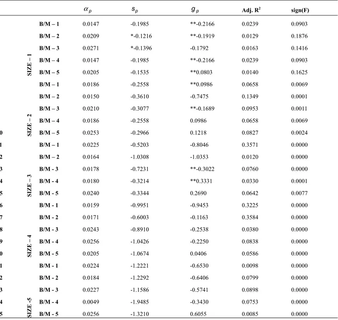
SMB and HML factors on their own cannot describe well portfolio excess returns (Table 7). F-test is almost always significant (except 5 portfolios), but R-squared is very poor: it exceeds 30% in only 3 portfolios and the others show R-squared always lower than 10% (except portfolio 7).
SMB regression coefficients are negative and decrease the larger the firm size. This means that sp is greater in
absolute value in portfolios of large firms. However, SMB coefficients are almost never statistically significant (only portfolios 2 and 3 show statistically significant coefficients at the 5% level). Portfolio excess returns are not therefore sensitive to the size premium.
Moving from low-B/M portfolios to high-B/M portfolios, HML coefficients gp tend to grow according to Fama and French (1993) but in 17 out of 25 portfolios they are not statistically significant. As a consequence, we cannot draw reliable conclusions about the effect of the value premium on the portfolio excess return.
Table 7.Time-series regressions: returns, SMB and HML
αp sp gp Adj. R2 sign(F) 1 SIZE – 1 B/M – 1 0.0147 -0.1985 **-0.2166 0.0239 0.0903 2 B/M – 2 0.0209 *-0.1216 **-0.1919 0.0129 0.1876 3 B/M – 3 0.0271 *-0.1396 -0.1792 0.0163 0.1416 4 B/M – 4 0.0147 -0.1985 **-0.2166 0.0239 0.0903 5 B/M – 5 0.0205 -0.1535 **0.0803 0.0140 0.1625 6 SIZE – 2 B/M – 1 0.0186 -0.2558 **0.0986 0.0658 0.0069 7 B/M – 2 0.0150 -0.3610 -0.7475 0.1349 0.0001 8 B/M – 3 0.0210 -0.3077 **-0.1689 0.0953 0.0011 9 B/M – 4 0.0186 -0.2558 0.0986 0.0658 0.0069 10 B/M – 5 0.0253 -0.2966 0.1218 0.0827 0.0024 11 SIZE – 3 B/M – 1 0.0225 -0.5203 -0.8046 0.3571 0.0000 12 B/M – 2 0.0164 -1.0308 -1.0353 0.0120 0.0000 13 B/M - 3 0.0178 -0.7231 **-0.3022 0.0760 0.0000 14 B/M - 4 0.0180 -0.3214 **0.3331 0.0330 0.0001 15 B/M - 5 0.0240 -0.3344 0.2690 0.0642 0.0077 16 SIZE – 4 B/M - 1 0.0159 -0.9951 -0.9453 0.3225 0.0000 17 B/M - 2 0.0171 -0.6003 -0.1163 0.3584 0.0000 18 B/M - 3 0.0243 -0.8910 -0.2538 0.0380 0.0000 19 B/M - 4 0.0256 -1.0426 -0.2250 0.0838 0.0000 20 B/M - 5 0.0205 -1.0674 0.0406 0.0586 0.0000 21 SIZE -5 B/M - 1 0.0224 -1.2221 -0.6530 0.0098 0.0000 22 B/M - 2 0.0184 -1.2292 -0.6406 0.0799 0.0000 23 B/M - 3 0.0227 -1.1586 -0.5741 0.0898 0.0000 24 B/M - 4 0.0049 -1.9485 -0.3430 0.0753 0.0000 25 B/M - 5 0.0256 -1.3210 0.6055 0.0085 0.0000 * Statistically significant at the 5% level.
** Statistically significant at the 10% level.
Table 7 reports the results of the regression model in which returns of each portfolio are regressed on SMB and HML factors. αp is the constant, sp is the SMB coefficient, gp is the HML coefficient, adj. R-squared measures the model goodness-of-fit, sign(F) is the F-test level of significance.
Regressions between portfolio risk premium, market risk premium, SMB, and HML
Table 8 shows the results of the third model, in which portfolio risk premium is regressed on market risk premium, SMB and HML simultaneously. The explanatory power of the model significantly improves and this is not due to collinearity between independent variables (Table 3, Panel A). We can draw the following main evidence:
-
β
p is positive and statistically significant (except portfolios 2, 9, and 10). This confirms that the market risk premium is a risk factor that should be included in the model.- sp is now statistically significant in almost all portfolios and seems to be positive for small portfolios (SIZE
- 1 and SIZE - 2) and negative for larger portfolios. This result is consistent with the presence of a small size effect in the financial industry too. Investors seem to require an additional risk premium to be disposed to hold small stocks.
- gp is not statistically significant only in 5 portfolios and, inside a size class, high-B/M portfolios show
higher regression coefficients than low-B/M portfolios. High-B/M firms seem to be more sensitive to the value premium and therefore pay a higher risk premium to investors that hold these stocks.
- Adjusted R-squared are significantly higher than those found in the previous two models. They are below 50% in 7 portfolios only, range between 50% and 70% in an additional 12 portfolios, and get to about 80% in the remainder 6 portfolios. Higher values concentrate on portfolios of large firms. Three-factor model appears to have a good power in explaining portfolio excess return variability in the financial sector.
- The constant of the model
α
p is never statistically different from zero, demonstrating that time-seriesvariations of returns are systematically explained by three risk premiums. Table 8. Time-series regressions: returns, market risk premium, SMB and HML
αp βp sp gp Adj. R2 F(sign) 1 SIZE – 1 B/M - 1 0.0020 *0.7700 0.3358 *0.1830 0.4779 0.0000 2 B/M - 2 0.0131 0.5325 *0.2494 0.0644 0.5627 0.0000 3 B/M - 3 0.0151 *0.7265 0.3646 *0.1979 0.5725 0.0000 4 B/M - 4 0.0020 *0.7700 *0.3358 *0.1830 0.4779 0.0000 5 B/M - 5 0.0101 *0.6315 *0.2849 *0.4082 0.5449 0.0000 6 SIZE – 2 B/M - 1 0.0099 *0.5279 *0.1105 *0.3726 0.5695 0.0000 7 B/M - 2 0.0026 *0.7514 *0.1604 -0.3574 0.4219 0.0000 8 B/M - 3 0.0113 *0.5868 0.0995 *0.1357 0.5238 0.0000 9 B/M - 4 0.0099 0.5279 *0.1105 *0.3726 0.4695 0.0000 10 B/M - 5 0.0146 0.6489 *0.1537 *0.4587 0.5928 0.0000 11 SIZE – 3 B/M - 1 0.0138 *0.5326 *-0.1507 *-0.5282 0.6180 0.0000 12 B/M - 2 0.0067 *0.5909 *-0.6208 *-0.7286 0.5950 0.0000 13 B/M - 3 0.0049 *0.7381 -0.1796 *0.1043 0.4664 0.0000 14 B/M - 4 0.0093 *0.5290 *0.0457 *0.6077 0.4742 0.0000 15 B/M - 5 0.0132 *0.6566 0.1213 *0.6098 0.3797 0.0000 16 SIZE – 4 B/M - 1 0.0028 *0.7963 *-0.4425 *-0.5319 0.8424 0.0000 17 B/M - 2 0.0066 *0.6378 *-0.1577 *0.2147 0.6421 0.0000 18 B/M - 3 0.0127 *0.7007 *-0.4047 0.1099 0.7901 0.0000 19 B/M - 4 0.0138 *0.7142 *-0.5470 0.1452 0.6532 0.0000 20 B/M - 5 0.0098 *0.7458 *-0.5540 *0.3998 0.6092 0.0000 21 SIZE – 5 B/M - 1 0.0143 *0.4944 *-0.8690 *-0.3963 0.8059 0.0000 22 B/M - 2 0.0074 *0.6641 *-0.7684 *-0.2958 0.8467 0.0000 23 B/M - 3 0.0117 *0.6670 *-0.6957 *-0.2279 0.7271 0.0000 24 B/M - 4 0.0058 *0.7284 *-1.4409 *0.0076 0.5176 0.0000 25 B/M - 5 0.0160 *0.6991 *-0.8530 0.9241 0.7387 0.0000 * Statistically significant at the 5% level
Table 8 reports the results of the regression model in which returns of each portfolio are regressed on market risk premium, SMB and HML factors. αp is the constant, β is the market risk premium coefficient, p sp is the SMB coefficient, gp is the HML coefficient, adj. R-squared measures the model goodness-of-fit, sign(F) is the
F-test level of significance. 5. Conclusions
In this study, we test the Fama-French three-factor model employed in the estimation of returns of financial stocks in Europe. The analysis shows the following main results:
- Market risk premium significantly affects stock returns in every model and its presence is required for the model to have a sufficient explanatory power. When it is used alone such as in the SL model, it works better in portfolios of large firms.
- Size and B/M are demonstrated to be cross-sectionally linked to stock returns: small firms and high-B/M firms show higher returns that market beta cannot explain.
- Size premium and value premium help explain time-series changes of returns only when they are used with the market risk premium. Regression coefficients sp and gp are almost always significantly different from zero in the three-factor model but not in the model that drops the market excess return.
- Investors require an extra return to small and high-B/M stocks that seem to be more sensitive to changes in the risk premium related to size and B/M factors.
In light of above results, financial stocks traded in the European stock exchanges yield returns that reward risks linked to small size and high B/M in addition to the market risk. This means that the need to price financial stocks may benefit from a multifactor model of risk in which size and B/M appear to be sources of risk like in non-financial industries. We do not want to mean that size and B/M necessarily proxy for the same risk sources as for non-financial firms but rather than being small and with a high B/M induces investors to ask for an additional risk premium in the financial sector too.
All of this has relevant implications for financial system and banking authorities. In the last decades, banks have diversified their revenue streams by significantly increasing proceeds generated by non-traditional, high-income activities such as investment banking. This, among other things, was the result of increased competition, deregulation, and financial market integration (e.g., Bessler and Kurmann, 2014). Moreover, the level of opaqueness of bank balance sheets has increased because of the expansion of complex and hard-to-value financial instruments and the rise of the originate-to-distribute model that took the place of the traditional, originate-to-hold model. Finally, bank leverage has increased significantly over the past 100 years (e.g., DeAngelo and Stulz, 2013) especially in large financial institutions.
These factors contributed to change bank risk exposure, made prudential rules on capital requirements outdated, and induced supervisors to introduce new frameworks for regulating capital adequacy, stress testing, and market liquidity risk. Banking authorities therefore require instruments to control for factors reflecting a large number of risks, from the traditional ones to the emerging ones. In this context, the use of market measures in the regulatory process, such as the book-to-market ratio and the market leverage, may help supervisory institutions assess bank risk exposure better.
While value premium seems to be relevant in estimating risk premium of financial and nonfinancial firms, the existence of a size premium is more ambiguous. In the financial sector, one can presume that large banks are more diversified and therefore less risky than smaller banks. However, the too big to fail policy may encourage irresponsible risk taking. The empirical evidence is mixed: some studies (e.g., Demsetz and Strahan, 1997) demonstrate that large and diversified banks work with less capital and undertake riskier projects, while some other (e.g., Konishi and Yasuda, 2004) finds a negative relationship between size and bank risk taking. More recent studies on size anomalies in US bank stock returns (Gandhi and Lustig, 2015) confirm that shareholders of large banks bear less risk and earn significantly lower risk-adjusted returns than those of small banks even though the former are significantly more leveraged than the latter. This evidence may be a result of government protections supporting large banks. We confirm this result and show that investors seem to require higher returns to smaller banks, but this point is still controversial (e.g., Goyal, 2017).
References
Allen, M. T., Madura, J., & Wiant, K. J. (1995). Commercial bank exposure and sensitivity to the real estate market. Journal of Real Estate Research, 10, 129-140. https://doi.org/10.5555/rees.10.2.952x8v34617g7006 Al-Mwalla, M., & Karasneh, M. (2011). Fama & French three factor model: Evidence from emerging market.
European Journal of Economics, Finance and Administrative Sciences, 41, 132-140.
Anwar, M., & Kumar, S. (2018). Three-Factor Model of Asset Pricing: Empirical Evidence from the Indian Stock Market. IUP Journal of Applied Finance, 24, 16-34.
Arshanapalli, B. G., Coggin, T. D., & Doukas, J. (1998). Multifactor asset pricing analysis of international value investment strategies. The Journal of Portfolio Management, 24, 10-23. https://doi.org/10.3905/jpm.1998.409650
Baek, S., Bilson, J. F. O. (2015). Size and value risk in financial firms. Journal of Banking and Finance, 55, 295-326. https://doi.org/10.1016/j.jbankfin.2014.02.011
Banz, R. (1981). The relationship between return and market value of common stocks. Journal of Financial Economics, 9, 3-18. https://doi.org/10.1016/0304-405X(81)90018-0
Barber, B. M., & Lyon, J. D. (1997). Firm size, book-to-market ratio, and security returns: A holdout sample of financial firms. The Journal of Finance, 52, 875-883. https://doi.org/10.1111/j.1540-6261.1997.tb04826.x Beaver, W., Kettler, P., & Scholes, M. (1970). The association between market determined and accounting
determined risk measures. Accounting Review, 45, 654-682.
Berk, J. (1995). A critique of size related anomalies. Review of Financial Studies, 8, 275-286. https://doi.org/10.1093/rfs/8.2.275
Bessler, W., & Booth, G. (1994). Interest rate sensitivity of bank stock returns in a universal banking system. Journal of International Financial Markets, Institutions, and Money, 3, 117-136.
Bessler, W., & Kurmann, P. (2014). Bank Risk Factors and Changing Risk Exposures: Capital Market Evidence Before and During the Financial Crisis. Journal of Financial Stability, 13, 151-166. https://doi.org/10.1016/j.jfs.2014.06.003
Bessler, W., & Murtagh, J. P. (2004). Risk characteristics of banks and non-banks: An international comparison. https://doi.org/10.1007/978-3-7908-2651-7_5
Bessler, W., Kurmann P., & Nohel, T. (2014). Time-Varying Systematic and Idiosyncratic Risk Exposures of US Bank Holding Companies. Journal of International Financial Markets, Institutions and Money, 35, 45-68. https://doi.org/10.1016/j.intfin.2014.11.009
Black, F. (1972). Capital market equilibrium with restricted borrowing. Journal of Business, 45, 444-455. https://doi.org/10.1086/295472
Black, F., Jensen, M. C., & Scholes, M. (1972). The capital asset pricing model: some empirical tests. In Jensen, M. C. (Ed.), Studies in the theory of capital markets (pp. 79-121). New York: Praeger Publishers, Inc. Brennan, M. J. (1970). Taxes, market valuation and corporate financial policy. National Tax Journal, 23, 417-427. Chamberlain, S., Howe, J. S., & Popper, H. (1997). The exchange rate exposure of US and Japanese banking institutions, Journal of Banking and Finance, 21, 871-892. https://doi.org/10.1016/S0378-4266(97)00002-2 Chan, K. C., & Chen, N. (1988). An unconditional asset pricing test and the role of firm size as an instrumental
variable for risk. Journal of Finance, 43, 309-325. https://doi.org/10.1111/j.1540-6261.1988.tb03941.x Chan, K. C., Karceski, J., & Lakonishok, J. (2000). New paradigm or same old hype in equity investing?,
Financial Analysts Journal, 56, 23-36. https://doi.org/10.2469/faj.v56.n4.2371
Chaudhary, P. (2017). Testing of three factor Fama-French model for Indian and US stock market. Journal of Commerce & Accounting Research, 6, 1-8
Choi, J. J., & Elyasiani, E. (1997). Derivative exposure and the interest rate and exchange rate risks of US banks, Journal of Financial Services Research, 12, 267-286. https://doi.org/10.1023/A:1007982921374
Choi, J. J., Elyasiani, E., Kopecky, K. (1992). The sensitivity of bank stock returns to market, interest and exchange rate risks. Journal of Banking and Finance, 16, 983-1004. https://doi.org/10.1016/0378-4266(92)90036-Y
Cohen, K. J., Hawawini, G. A., Maier, S. F., Schwartz, R. A., & Whitcomb, D. K. (1983). Estimating and Adjusting for the Intervalling-Effect Bias in Beta. Management Science, 29, 135-148. https://doi.org/10.1287/mnsc.29.1.135
Daniel, K., & Titman, S. (1997). Evidence on the characteristics of cross sectional variation in stock returns. The Journal of Finance, 52, 1-33. https://doi.org/10.1111/j.1540-6261.1997.tb03806.x
Davis, J. L., Fama, E. F., & French, K. R. (2000). Characteristics, covariances, and average returns: 1929 to 1997, The Journal of Finance, 55, 389-406. https://doi.org/10.1111/0022-1082.00209
DeAngelo, H., Stulz, R. M. (2013). Why high leverage is optimal for banks. NBER Working Paper No. 19139. https://doi.org/10.3386/w19139
Demsetz, R. S., & Strahan, P. E. (1997). Diversification, size, and risk at bank holding companies. Journal of Money, Credit and Banking, 29, 300-313. https://doi.org/10.2307/2953695
Dewenter, K. L., & Hess, A. C. (1998). An international comparison of banks’ equity returns. Journal of Money, Credit and Banking, 30, 472-492. https://doi.org/10.2307/2601251
Dimson, E., & Marsh, P. (1999), Murphy’s law and market anomalies. Journal of Portfolio Management, 25, 53-69. https://doi.org/10.3905/jpm.1999.319734
Drobetz, W., Erdmann, T., & Zimmermann, H. (2007). Predictability in the cross-section of European bank stock returns. WWZ Working Paper.
Eraslan, V. (2013). Fama and French Three-Factor Model: Evidence from Istanbul Stock Exchange. Business and Economics Research Journal, 4, 11-22.
Fama, E. F., & French, K. R. (1992). The cross-section of expected stock returns. The Journal of Finance, 47, 427-465. https://doi.org/10.1111/j.1540-6261.1992.tb04398.x
Fama, E. F., & French, K. R. (1993). Common risk factors in the returns on stocks and bonds, Journal of Financial Economics, 33, 3-56. https://doi.org/10.1016/0304-405X(93)90023-5
Fama, E. F., & French, K. R. (2015). A five-factor asset pricing model. Journal of Financial Economics, 116, 1-22. https://doi.org/10.1016/j.jfineco.2014.10.010
Fama, E. F., & French, K. R., (2016). Dissecting Anomalies with a Five-Factor Model. Review of Financial Studies, 29, 69-103. https://doi.org/10.1093/rfs/hhv043
Fama, E. F., French, K. R. (2017). International tests of a five-factor asset pricing model. Journal of Financial Economics, 123, 441-463. https://doi.org/10.1016/j.jfineco.2016.11.004
Fama, E. F., MacBeth, J. (1973). Risk, return and equilibrium: empirical tests. The Journal of Political Economy, 81, 607-636. https://doi.org/10.1086/260061
Fama, E.F., French, K.R., 2012, Size, value, and momentum in international stock returns. Journal of Financial Economics 105, 457-472. DOI: 10.1016/j.jfineco.2012.05.011
Flannery, M. J., James, C. M. (1984). The effect of interest rate changes on the common stock returns of financial institutions. The Journal of Finance, 39, 1141-1153. https://doi.org/10.1111/j.1540-6261.1984.tb03898.x Foye, J., Mramor, D., Pahor, M. (2013). A respecified Fama French three-factor model for the new European
Union member states. Journal of International Financial Management & Accounting, 24, 3-25. https://doi.org/10.1111/jifm.12005
Gandhi, P., & Lustig, H. (2015). Size anomalies in US bank stock returns, The Journal of Finance, 70(2), 733-768. https://doi.org/10.1111/jofi.12235
Gibbons, M. R. (1982). Multivariate tests of financial models: a new approach. Journal of Financial Economics 10(1), 3-27. https://doi.org/10.1016/0304-405X(82)90028-9
Giliberto, M. (1985). Interest rate sensitivity in the common stocks of financial intermediaries: a methodological note, Journal of Financial and Quantitative Analysis, 20, 123-126. https://doi.org/10.2307/2330682
Gounopoulos, D., Molyneux, P., Staikouras, S. K., Wilson, J. O. S., & Zhao G. (2013). Exchange rate risk and the equity performance of financial intermediaries, International Review of Financial Analysis, 29, 271-282. https://doi.org/10.1016/j.irfa.2012.04.001
Griffin, J. M. (2002). Are the Fama and French factors global or country specific? Review of Financial Studies, 15, 783-803. https://doi.org/10.1093/rfs/15.3.783
Hess, A. C., & Laisathit, K. (1997). A market-based risk classification of financial institutions, Journal of Financial Services Research, 12, 133-158. https://doi.org/10.2139/ssrn.978
Hong, K. J., & Satchell, S., (2014). The sensitivity of beta to the time horizon when log prices follow an Ornstein– Uhlenbeck process. The European Journal of Finance, 20(3), 264-290. https://doi.org/10.1080/1351847X.2012.698992
Horowitz, J. L., Loughran, T., Savin, N. E. (1999). The disappearing size effect, Research in Economics, 54(1), 83-100. https://doi.org/10.1006/reec.1999.0207
Horowitz, J. L., Loughran, T., Savin, N. E. (2000). Three analyses of the firm size premium. Journal of Empirical Finance, 7, 143-153. https://doi.org/10.1016/S0927-5398(00)00008-6
Jones, S. L., & Yeoman, J. C. (2012). Bias in estimating the systematic risk of extreme performers: Implications for financial analysis, the leverage effect, and long-run reversals. Journal of Corporate Finance, 18(1), 1-21. https://doi.org/10.1016/j.jcorpfin.2011.09.007
Kane, E. J., & Unal, H. (1988). Change in market assessments of deposit-institution riskiness. Journal of Financial Services Research, 1, 207-229. https://doi.org/10.1007/BF00114851
Konishi, M., & Yasuda, Y. (2004). Factors affecting bank risk taking: Evidence from Japan. Journal of Banking and Finance, 28, 215-232. https://doi.org/10.1016/S0378-4266(02)00405-3
Kothari, S. P., Shanken, J., & Sloan, R. (1995). Another look at the cross-section of expected stock returns. The Journal of Finance, 50, 185-224. https://doi.org/10.1111/j.1540-6261.1995.tb05171.x
Lindenberg, E. (1979). Capital market equilibrium with price affecting institutional investors. In Elton, E. J., Gruber, M. J. (Eds.), Portfolio theory 25 years after. Amsterdam: North-Holland Publishing Company. Lintner, J. (1965). The valuation of risk assets and the selection of risky investments in stock portfolios and capital
budgets. Review of Economics and Statistics, 47, 13-37. https://doi.org/10.2307/1924119
Lynge, M. J., & Zumwalt, J. K. (1980). An empirical study of the interest rate sensitivity of commercial bank returns: A multi-index approach. Journal of Financial and Quantitative Analysis, 15, 731-742. https://doi.org/10.2307/2330406
Manjunatha, T., & Mallikarjunappa, T. (2011). Does three-factor model explain asset pricing in Indian capital market? Decision, 38, 119-140.
Martins, A. M., Serra, A. P., & Martins, F. V. (2012). Real estate market risk in bank stock returns: Evidence for 15 European countries. Working Paper, University of Porto.
Mayers, D. (1972). Nonmarketable assets and capital market equilibrium under uncertainty. In Jensen, M. C. (Ed.), Studies in the theory of capital markets. New York: Praeger Publishers, Inc.
Mayshar, J. (1981). Transaction costs and the pricing of assets, The Journal of Finance 36, 583-597. https://doi.org/ 10.1111/j.1540-6261.1981.tb00646.x
Mei, J., & Saunders, A. (1995). Bank risk and real estate: An asset pricing perspective, Journal of Real Estate Finance and Economics, 10, 199-224. https://doi.org/10.1007/BF01096939
Miller, M., Scholes, M. (1972). Rates of return in relation to risk: a re-examination of some recent findings. InJensen, M. C. (Ed.), Studies in the theory of capital markets. New York: Praeger Publishers, Inc.
Modigliani, F., & Miller, M. (1958). The cost of capital, corporation finance and the theory of investment. The American Economic Review, 48(3), 261-297.
Modigliani, F., & Miller, M. (1963). Corporate income taxes and the cost of capital: a correction. The American Economic Review, 53(3), 433-443.
Moerman, G. A. (2005). How domestic is the Fama and French three-factor model? An application to the Euro area, ERIM Report Series Reference No. ERS-2005-035-F&A.
Mossin, J. (1966). Equilibrium in a capital asset market. Econometrica, 34, 768-783. https://doi.org/10.2307/1910098
Oertmann, P., Rendu, C., & Zimmermann, H. (2000). Interest rate risk of European financial corporations, European Financial Management, 6, 459-478. https://doi.org/10.1111/1468-036X.00135
Roll, R. (1977). A critique of the Asset Pricing Theory’s tests: Part I: on past and potential testability of the theory, Journal of Financial Economics, 4, 129-176. https://doi.org/10.1016/0304-405X(77)90009-5
Ross, S., 1976, The arbitrage theory of capital asset pricing, Journal of Economic Theory 13(3), 341-360. https://doi.org/10.1016/0022-0531(76)90046-6
Schuermann, T., & Stiroh, K. J. (2006). Visible and hidden risk factors for banks. Staff Report Nr. 252, Federal Reserve Bank of New York.
Sehgal, S., & Balakrishnan, A. (2013). Robustness of Fama-French three factor model: further evidence for Indian stock market. Vision: The Journal of Business Perspective, 17, 119-127. https://doi.org/10.1177/0972262912483526
Sharma, R., & Mehta, K. (2013). Fama and French: Three Factor Model. Journal of Indian Management, 1, 90-105.
Sharpe, W. F. (1964). Capital asset prices: a theory of market equilibrium under conditions of risk. The Journal of Finance, 19, 425-442. https://doi.org/10.2307/2977928
Stambaugh, R. F. (1982). On the exclusion of assets from tests of the two-parameter model: a sensitivity analysis. Journal of Financial Economics, 10(3), 237-268. https://doi.org/10.1016/0304-405X(82)90002-2
Taneja, Y. P. (2010). Revisiting Fama French three-factor model in Indian stock market. Vision: The Journal of Business Perspective, 14, 267-274. https://doi.org/10.1177/097226291001400403
Treynor, J. (1962). Toward a theory of the market value of risky assets, unpublished manuscript. https://doi.org/10.1002/9781119196679.ch6
Viale, A. M., Kolari, J. W., & Fraser, D. R. (2009). Common risk factors in bank stocks, Journal of Banking and Finance, 33, 464-472. https://doi.org/10.1016/j.jbankfin.2008.08.019
Copyrights
Copyright for this article is retained by the author(s), with first publication rights granted to the journal.
This is an open-access article distributed under the terms and conditions of the Creative Commons Attribution license (http://creativecommons.org/licenses/by/4.0/).