Variable length pendulum analyzed by a comparative
Fourier and wavelet approach
M.T. Caccamoa, S. Magaz`ua,b,∗
aDepartment of Mathematical and Informatics Sciences, Physical Sciences and Earth Sciences of Messina University, Viale Ferdinando Stagno D’ Alcontres 31, 98166 Messina, Italy.
bLe Studium, Loire Valley Institute for Advanced Studies,
Orl´eans & Tours, France, CBM (CNRS), rue Charles Sandron, 45071 Orl´eans, France. *e-mail: [email protected]
Received 14 July 2017; accepted 10 November 2017
The motion of a pendulum with a variable length is analyzed by means of a comparative Fourier and Wavelet approach. In particular Fourier and continuous Wavelet transforms have been jointly employed to investigate the non stationary signal of a variable length pendulum in an easy-to-interpret scenario addressed to undergraduate and graduate students. The comparison between the two data analysis protocols allows to easily show that while the Fourier transform is able to extract only an average frequency value for the variable length pendulum motion, Wavelet analysis furnishes information on the time behaviour of the motion spectral content, i.e. provides a joint time-frequency analysis.
Keywords: Variable length pendulum; Fourier transform; wavelet transform.
PACS: 01.40.Fk; 01.50.pa; 02.30.Nw
1.
Introduction
The basic assumption of this work is to show how, in teaching and learning Mathematics and Physics, the close interrela-tion between the two disciplines and with Laboratory should not be circumvented or bypassed. On the contrary their in-terplay and mutual influence as well as their deep episte-mological affinities should be promoted. In this framework Mathematics does not just provide tools for Physics but also drives physical insight; vice-versa Physics and its Labora-tory can provide a simple access to Mathematical topics of not straighforward comprehension. Recent student learning investigations suggest that the understanding of Physics and Mathematics topics can be significantly facilitated by means of an integrated approach (see Fig. 1) with Laboratory activ-ities, so allowing to enreach topics of meanings.
In other words, in undergraduate and graduate courses, disciplines as Physics and Mathematics are frequently set in an autonomous way by means of the delimitation of their frontiers, the building of specialistic languages and the em-ployment of specific techniques and tools; such an approach furnishes points of strength to the single disciplines but at the same time furnishes the limits of the disciplinary knowledge. Disciplines are observation windows on the World, points of view on reality but if disciplines forget to be a part of a wider system of knowledge the interdisciplinary boundary limits become barriers and, in such a case, the word discipline re-cover its original meaning of whip for who intends to break the disciplinary walls.
In this reference contest, due to complexities encoun-tered in dealing with time dependent frequencies, the study of variable length pendula as well as the study of Fourier and Wavelet transforms are rarely included within the program
FIGURE1. In undergraduate and graduate courses, Physics, Lab-oratory and Mathematics often tend to be autonomous through the delimitation of their frontiers and the building of specialistic lan-guages. An open dialogue among Mathematics, Physics and Lab-oratory allows to confer to formal issues concrete form and utility and vice-versa allows to provide effective analysis tools to physical insights.
of Physics courses addressed to ungraduate and graduate stu-dents.
Such physical systems are characterized by a chirp-like time behavior, i.e. by local (i.e. time-dependent) pseudo-frequencies [1,2].
In the present work it will be shown how while Fourier Transform (FT) reveals an effective tool in analyzing
station-82 M.T. CACCAMO AND S. MAGAZ ´U
ary signals, in the presence of a time changing spectral con-tent FT is not able to furnish detailed information on the dif-ferent physical states of the oscillating system but provides only an average information on the motion frequency com-ponents; on the contrary in this latter case Wavelet Trans-form (WT) represents an effective tool for the time analysis of the non stationary signal allowing to precisely characterize the time variation of the oscillation motion frequency con-tent [3-5]. WT is nowadays extensively used in several fields of applications, such as audio, images, light and neutron scat-tering spectra analysis, spectroscopy, geophysics time series, biology and medicine [6-16].
In the following, in order to analyse the dynamics of a pendulum with a time-varying length, we apply both the FT with the WT approaches putting into evidence the pros et cons of the two analysis techniques.
2.
Comparison between Fourier and wavelet
transforms - historical background
From the historical point of view it is useful to mention that in 1822, Joseph Fourier, French mathematician and physicist who accompanied Napoleon on his Egyptian campaign, pub-lished the treatise titled “Theorie Analytique de la Chaleur” where he introduced the idea of expanding functions in sine or cosine trigonometric series to solve the heat conduction equation he had developed.
Starting from this study, FT allows to decompose a signal and to reconstruct it without loss of information even if such an analysis is localized in frequency but not in time; in other words FT allows to properly analyse stationary signals [17].
In order to overcome the limitations of FT a new analy-sis has been introduced later; such an analyanaly-sis conanaly-sists in in-troducing a “window” function of given length which slides along the time axis to execute a “time-localized” FT. This approach gives rise to the Short Time Fourier Transform (STFT) which was first introduced in 1946 by Dennis Gabor, a Hungarian mathematician. Gabor chose as window func-tion a Gaussian but soon he realized that STFT furnished an equal resolution in time for lower and higher frequencies and that the width of the window function was the same for the entire analysis process [18].
In the mid 1970s Jean Morlet, a French geophysics work-ing for an oil company, while investigatwork-ing the acoustic echoes sent into the soil for identifying the existence of oil on the earth’s crest, developed the method of scaling and shift-ing the STFT. In order to analyse such echoes, Morlet first employed the STFT and observed that when holding constant the width of the window function the analysis didn’t run well; so, he proposed to maintain fixed the frequency of the win-dow function and to change the width of the winwin-dow by a dilatation or compression procedure [19].
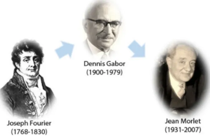
This new approach led to the term “ondelette” introduced by Jean Morlet et Alex Grossmann in 1984. At first, the term was French and then was translated in English as wavelet:
FIGURE2. Historical route of the Wavelet genesis which starting from Joseph Fourier with FT (1822), through Dennis Gabor with FTFT (1946), arrives to Jean Morlet (1984) with WT.
i.e. wave (onde) and let (petite). Figure 2 shows the histori-cal route of the wavelet concept genesis which starting from Joseph Fourier with FT (1822), through Dennis Gabor with STFT (1946), arrives to Jean Morlet (1984) with WT.
From a mathematical point of view Fourier series allow to decompose a periodic function f (x) defined for 0 ≤ x ≤ 2π into a sum of sine or cosine functions [20,21]:
f (x) ∼ a0 2 + ∞ X k=1 [akcos(kx) + bksin(kx)] (1)
where a0, akand bkare the Fourier coefficient, defined as:
a0= 1 2π 2π Z 0 f (x)dx; (2) ak = 1 π 2π Z 0 f (x)dx cos(kx); (3) bk = 1 π 2π Z 0 f (x)dx sin(kx); (4)
Figure 3 shows, as an example, the partial sums of the Fourier series for a square wave.
The Fourier Transform is an extension of the Fourier se-ries to non-periodic functions which decompose it into a set of sine (or cosine) waves of different frequencies ω:
ˆ f (ω) = ∞ Z −∞ f (t)e−iωtdt, (5)
It should be stressed that in such a case it is not possible to provide a connection between the frequency spectrum and the signal evolution in time.
On this regard, WT results more advantageous in respect to Fourier transform; in fact WT approach allows to decom-pose a signal into its wavelets components, by means of mother wavelet ψ:
FIGURE3. Partial sums of the Fourier series for a square wave. fψ(a, τ ) = √1 a ∞ Z −∞ f (t)ψ ∗ µ t − τ a ¶ dt (6)
where the parameter a > 0 denotes the scale and its value is the inverse of the frequency; the parameter τ represent the shift of the scaled wavelet along the time axis. ψ∗ represents the complex conjugation of the wavelet while the mother wavelet ψ can be expressed by [22]:
ψa,τ(t) = √1 aψ µ t − τ a ¶ (7) In Fig. 4, as an example, scaled and shifted versions of the mother wavelet are reported.
Differently from FT, which shows only which signal fre-quencies are present, WT, in addition, also shows where, or at
what scale they are. Furthermore, while FT allows to decom-pose the signal only in cosine and sine component functions, the WT takes into account several wavelet mother functions, that can be chosen according to the similarity degree of the mother functions with the investigated signal [23-30] .
In this paper, according to the behavior of the investigated oscillator, the wavelet Morlet has been chosen as mother wavelet: ψ(t) = e ³ iω0−2σ2t2 ´ (8) where ω0represents the center pseudo-frequency and ?
pro-vides the wavelet bandwidth [31].
It should be noticed that in the special case in which the wavelet mother is ψ(t) = e−2πit the WT transform reduces to the FT.
84 M.T. CACCAMO AND S. MAGAZ ´U
FIGURE4. Scaled and shifted versions of the mother wavelet
3.
Theoretical background
Let us first focus the attention on a pendulum, a toy physics system full of lots of meanings (see Fig. 5), of length `(t) whose mass is m in the absence of any friction.
From the physical point of view the dynamics of such a system can be obtained by applying the fundamental second law equation dynamics equation:
m~a = ~F (9)
m¨s = −mg sin θ (10) where a is the acceleration, F is the total force acting on the mass, θ is the pendulum angular deviation from the equilib-rium position, s = `(t)θ(t) is the length spanned by the
oscil-FIGURE5. Pendulum as represented by Lucia Grasso painter.
lation during its motion, ¨s = d2s/dt2is its second derivative, and finally g is the gravity acceleration [32-37].
Being: s(t) = `(t)θ(t) (11) it results: ˙s(t) = ˙`(t)θ(t) + `(t) ˙θ(t) (12) and ¨ s = ¨`θ + ˙` ˙θ + ˙` ˙θ + `¨θ = ¨`θ + 2 ˙` ˙θ + `¨θ (13) Under the hypothesis that the pendulum length during the oscillation changes with a constant rate, i.e. ˙` = const., it is:
¨
` = (d2`)/(dt2) = 0. Furthermore if one can assume that,
during the oscillation, the pendulum length `(t) changes in time slowly in respect to the θ(t) time changes, i.e. ˙` ¿ ˙θ, one can ¨s = `¨θ [38-41].
Under these assumption, Eq. (10) becomes:
m`(t) ¨θ(t) = −mg sin θ(t) (14) and making the further assumption that θ(t) ¿ 1 and hence sin θ(t) ∼ θ(t), it results:
¨
θ(t) = − g
`(t)θ(t) (15)
whose solution can be put under the form:
θ(t) = θ0sin(ω(t)t + ϕ) (16) where: ω(t) ≈ r g l(t) (17)
4.
The experimental setup and results
The experimental set-up includes:• a spherical mass whose weight is 100 g; • a fixed support to fix the pendulum;
• a step by step rotating device for changing the
pendu-lum length;
• a computer equipped with data acquisition program
(Logger Lite) and spreadsheet (Excel);
• an ultrasonic sensor device to measure the distance
be-tween itself and the oscillating mass which directly transmit the recorded data to a PC.
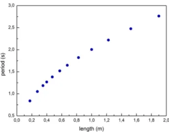
FIGURE6. Behavior of the oscillation period T as a function of the pendulum length under stationary conditions.
FIGURE7. Length variation versus time. The pendulum length as a function of time fulfils an linear trend with a slope of -0.025 m/s.
FIGURE 8. Comparison of the investigated signal analyzed by means of FT and WT. More precisely, on the top of the figure the collected oscillation signal, under the condition of varying length is shown; on the right of the figure its FT showing only an aver-age of the registered signal frequencies; on the bottom of the figure the WT scalogram that shows how the oscillation pseudo-frequency changes with time.
As far as the experiment procedure is concerned, the pen-dulum motion was sampled through a GoMotion-Vernier sen-sor. The system length variation as a function of time was assured by the step by step rotating device and was registered through a PC.
During the first part of the experience, the condition in which the pendulum length is fixed was investigated, reiter-atly registering the motion at different pendulum lengths. The oscillation period evaluated for different lengths is reported in Fig. 6 that, as expected, fulfills the expected T = 2πpl/g
law.
First, we have studied the system under stationary condi-tions, i.e. at fixed pendulum length, and then we have inves-tigated and the analyzed, by a WT approach, a set of mea-surements in which the length changed linearly as a function of time [42-45,39-40]. In Fig. 7, as an example, the length variation versus time plot is reported. As it can be seen the pendulum length as a function of time fulfils a linear trend with a constant slope of ∆l/∆t = 0.025 ms−1.
Figure 8 reports a picture of the analyzed signal. In par-ticular, on the top, the collected oscillation signal in the con-dition of length change is shown. It is clear that oscillation frequency increases with time. FT, that is reported on the right of the picture, provides only an average of the frequen-cies of the investigated signal; while, on the bottom of the picture, the WT scalogram shows that the oscillation pseudo-frequency changes with the time.
5.
Conclusion
The present paper shows an example of how it is possible to promote a fruitful alliance among different disciplines on a specific study case which allows to access in an user-friendly way to mathematical operations such as Fourier and Wavelet transforms. Both these approaches have been applied to char-acterize the effects of the pendulum length change on the following time-dependent oscillation frequency. It is shown that WT outperforms the FT approach highlighting which frequencies are present (as FT) and, in addition, where they are, so providing an easy-to-interpret physical significance of time-frequency analysis.
86 M.T. CACCAMO AND S. MAGAZ ´U
1. R.A. Carmona, W.L. Hwang, and B. Torresani, IEEE Trans.
Signal Process. 47 (1999) 480-492.
2. A. Arneodo, E. Bacry, and J.F. Muzy, Phys. Rev. Lett. 74 (199)
4823-4826.
3. M.T. Caccamo and S. Magaz`u, Eur. J. Phys. 38 (2017). 4. I. Daubechies, IEEE Trans. Inf. Theory 36 (1990).
5. L. Debnath, Fourier Transforms and Their Applications in
Wavelet Transforms and Their Applications (Boston, MA:
Birkh¨auser Boston, 2002).
6. H. Adeli, Z. Zhou, and N. Dadmehr, J. Neurosci. Methods 123
(2003) 69-87.
7. A. Arn´eodo, N. Decoster, P. Kestener, and S.G. Roux, Adv.
Imaging Electr. Phys. (2003) 1-92.
8. S. Magaz`u, F. Migliardo, and M.T. Caccamo, J. Phys. Chem. B
116 (2012) 9417-9423.
9. F. Migliardo, M. T. Caccamo, and S. Magaz`u, Food Biophys. 9
(2014) 99-104.
10. S. Magaz`u, F. Migliardo, B.G. Vertessy, and M.T. Caccamo,
Chem. Phys. 424 (2013) 56-61.
11. F. Migliardo, S. Magaz¨´, and M.T. Caccamo, J. Mol. Struct.
1048 (2013) 261-266.
12. M.T. Caccamo and S. Magaz`u, Vib. Spectrosc. 85 (2016)
222-227.
13. X.-G. Miao and W.M. Moon, Geosci. J. 3 (1999) 171-179. 14. A. Prokoph and R.T. Patterson, Atmosphere-Ocean. 42 (2004)
201-212.
15. A. Arneodo, C. Vaillant, B. Audit, F. Argoul, Y.
d’Aubenton-Carafac, and C. Thermesc, Phys. Rep. 498 (2011) 45-188.
16. E. Gerasimova et al., Front. Physiol. 5 (2014) 176.
17. J.-B.-J. Fourier, The analytical theory of heat (Cambridge
Uni-versity Press, 2009).
18. D. Gabor, J. Inst. Elec. Eng. 93 (1946) 429-457.
19. J. Morlet, G. Arens, E. Fourgeau, and D. Glard, Geophysics 47
(1982) 203-221.
20. G.B. Arfken and H.-J. Weber, Mathematical methods for
physi-cists (Academic Press, 1995).
21. T.W. K¨orner, Fourier analysis (Cambridge University Press,
1988).
22. C. Torrence and G.P. Compo, Bull. Am. Meteorol. Soc. 79
(1998) 61-78.
23. A. Graps, IEEE Comput. Sci. Eng. 2 (1995) 50-61.
24. M. T. Caccamo and S. Magaz`u, Spectrosc. Lett. 50 (2017)
130-136.
25. N. Ahuja, S. Lertrattanapanich, and N.K. Bose, IEE Proc. -
Vi-sion, Image, Signal Process. 152 (2005) 659.
26. A.W. Galli, G.T. Heydt, and P.F. Ribeiro, IEEE Comput. Appl.
Power 9 (1996) 37-41.
27. S. Magaz`u, F. Migliardo, and M.T. Caccamo, Adv. Mater. Sci.
Eng. (2013).
28. M. B. Priestley, J. Time Ser. Anal. 17 (1996) 85-103.
29. M.T. Caccamo and S. Magaz`u, Appl. Spectrosc. 71 (2017)
401-409.
30. S.G. Mallat, IEEE Trans. Pattern Anal. Mach. Intell. 11 (1989)
674-693.
31. J. Morlet, G. Arens, E. Fourgeau, and D. Giard, Geophysics, 47
(1982) 222-236.
32. R.A. Serway, R.J. Beichner, and J.W. Jewett, Physics for
scien-tists and engineers. (Brooks/Cole-Thomson Learning, 2000).
33. X. Xin and Y. Liu, Commun. Nonlinear Sci. Numer. Simul. 19
(2014) 1544-1556.
34. I.T. Osmond, Science 22 (1905) 311-312. 35. L.D. Patterson, Osiris 10 (1952) 277-321.
36. M. Delgado, A. Portnoy, and J.A. Fuquene, Rev. Bras. Biom. 24
(2010) 66-84.
37. L.D. Akulenko and S.V. Nesterov, J. Appl. Math. Mech. 73
(2009) 642-647.
38. R.P. Feynman, R.B. Leighton, and M.L. Sands, The Feynman
lectures on physics. Reading Mass.: (Addison-Wesley Pub. Co,
1963).
39. M.S. Tiersten, Am. J. Phys. 37 (1969) 82-87.
40. A. Sommerfeld, Chapter I - Thermodynamics. General
Consid-erations, in Lectures on Theoretical Physics, (Academic Press,
1964).
41. S. Gil and E. Rodr´ıguez, F´ısica re-creativa: experimentos de
f´ısica usando nuevas tecnolog´ıas. (Prentice-Hall, 2001).
42. V.K. Gupta, G. Shanker, and N.K. Sharma, Am. J. Phys. 54
(1986) 619-622.
43. P.T. Squire, Am. J. Phys. 54 (1986) 984-991.
44. X.-J. Wang, C. Schmitt, and M. Payne, J. Phys. 23 (2002)
155-164.
45. A. Arneodo, E. Bacry, S. Jaffard, and J.F. Muzy, J. Fourier