Climate Change Threatens Coexistence within Communities of Mediterranean Forested Wetlands

(1)

UNIVERSITA‘ DEGLI STUDI DELLA TUSCIA

DIPARTIMENTO

PER L‘INNOVAZIONE NEI SISTEMI BILOGICI, AGROALIMENTARI E FORESTALI

(DIBAF)

Corso di Dottorato di Ricerca in ECOLOGIA FORESTALE

XXIV° ciclo

Settore scientifico disciplinare AGR/05

Climate Change Threatens Coexistence within Communities of

Mediterranean Forested Wetlands

Coordinatore: Dottorando:

Prof. Paolo De Angelis Arianna Di Paola

Tutor: Cotutor:

(2)

(3)

ABSTRACT

Mediterranean basin supports characteristic Mediterranean forests, woodlands, and scrub vegetation, highly adapted to the mild, rainy winters and hot, dry summers that characterize the Mediterranean climate. Never less the Mediterranean region has been identified as one of the hot spots of climate change. This study aims to understand what are the conditions of coexistence, thus biodiversity, of Mediterranean tree species in humid areas under future scenarios of altered hydrological regimes. The core of the work is a quantitative, dynamic model exploring the coexistence of different mediterranean tree species, typical of the arid or semi-arid wetland where ecological overlaps exist between mesic communities and those dominated by wetland specialists. The original idea of the paper is to address this topic from a deterministic approach using a dynamical model which is validated by existing data on species abundance. The dynamic of the population is broadly-defined according to the distinct adaptive strategies of trees for water stress of summer drought and winter flooding while climate change are explored as external forcing by means of a bifurcation analysis and compared with the major regional climate scenarios.

I argue that at intermediate levels of water supply, which do not benefit either of the two species, the dual role of water (resource and stress) results in the coexistence of two kind of species, namely Hygrophilous and Non-hygrophilous. In order to support the validity of the ideas contained in the present study I applied the model to a Mediterranean coastal forested wetlands of Central Italy located into Castelporziano Estate and Circeo National Park.

The results obtained show that there are distinct rainfall thresholds on the ability of Mediterranean wetlands to maintain species coexistence and hence to sustain biodiversity, calling for an urgent adaptation and mitigation response to prevent human pressure on water resources in proximity of wetland forested areas.

(4)

1. INTRODUCTION

The present thesis deals with dynamic models of wet forest systems. This chapter is devoted to a short introduction about regime shift, resilience and dynamic models in ecological system. In order to justify my choices and my goals I will do an overview of the main issues addressed and the methodology used.

1.1 Aim of the thesis

The aim of this thesis is to develop a competition model that allows for coexistence between trees, or groups of trees, having distinct adaptative strategies for water stress. My purpose is to represent the minimal set of physiological behaviour, by a simple mathematical model, that I believe is central for understanding how coexistence arises and is maintained in transitional forested wetlands.

The main objective is to use the model with an analytic approach as a tool for assessing the resilience to climate changes of states of coexistence of different plants type. In other words, I aim to identify the parameter boundaries within which biodiversity is preserved. For this purpose I have first identified the equilibria of the system and outlined their stability, then I have determined the bifurcation points for changing climatic inputs.

Along an hydric gradient, when water is abundant, hygrophilous species, or drought-sensitive types, have a much higher rate of CO2 assimilation, thus growing rates,

together with higher transpiration rates compared to non-hygrophilous ones (Schulze, 2005; Brian and Hicks, 1982). As soil dries non-hygrophilous types should increase water use efficiency so that under this condition non-hygrophilous types dominate (Schulze, 2005).

I argue that at intermediate levels of water supply, which do not benefit either of the two species, the dual role of water (resource and stress) results in the coexistence of these two kind of species.

These topics are of importance both from a theoretical and practical point of view: understanding the mechanisms that support coexistence into natural system could help to determine the main interactions that have to be considered in more complex

(7)

2

predictive models. At the same time, assessing the resilience to climate changes of ecosystems would provide practical information to decision makers to improve management decisions.

In order to support the validity of the ideas contained in the present study I applied the model to a Mediterranean coastal forested wetland of Central Italy (located in the Presidential Park of Castelpoziano Estate and Circeo National Park). This choice has two reasons: (i) this wet forest ecosystem are characterized by high biodiversity and presence of endemism; (ii) despite their strong anthropogenic changes and reduced extension (Presti et al., 1998, Stanisci et al., 1998) they have never been included in Europe's most threatened natural ecosystems and are not listed in Annexe I of the European Habitats Directive as being a priority forest habitat type.

However this model is generally applicable to the wet ecotones on arid and semi-arid areas where water is the main limiting factor and where sharp ecological gradients exist between more xeric upland communities and those dominated by wetland specialists.

1.1.1 Model Competitors

In arid and semi-arid wetlands or wherever plants are subjected to alternate periods of summer drought and winter flooding like some sites of the Mediterranean basin, the main resource for which plants compete - namely, water - is also a major stress factor that effects distinct types of plants at distinct times of the year (Rodiriguez Gonzales et al., 2010; Gasith and Resh, 2009). A review of possible adaptive strategies to water stress factors is beyond the scope of this work. Detailed bibliography on the effects of water stress is very rich (Van der Molen et al., 2011, Kozloswsky, 1997).

Here we refer to the water use efficiency as the ratio between the plant growth rate and the plant water use, or lost by transpiration. Drought and flooding are generally avoided by several physiological acclimations that, respectively and overall, increase plants water use efficiency or provide a continuous source of water over the growing season and that allows plants to withstand the root asphyxia (Rodiriguez Gonzales et al., 2010; Schulze, 2005; Van Der Molen et al., 2011; Kozlowsky, 1997). Briefly speaking, the two types of water stress with the respective strategies can be summarized as follows:

(8)

3

 Root-anoxia stress during the wet periods. Some hygrophilous plants can survive to water logging by complex interactions of morphological, anatomical, and physiological adaptations (Kozlocvsky, 1997). Important adaptations include production of hypertrophied lenticels, aerenchyma tissue, and adventitious roots. These facilitate the movement of oxygen from leaves and stems to roots, thus permitting them to function in an oxygen-deficient environment (Kozlocvsky, 1997; Van Der Molen et al., 2011). When the flood water drains away, plants may be less drought tolerant because of their low root/shoot ratios (Kozlocvsky, 1997 );

 Drought-stress tolerant during the summer. Plants are developmentally and physiologically designed by evolution to reduce water use under drought stress (Schulze, 2005; Blum, 2005). physiological responses of the vegetation to drought include reductions in enzymatic activities as well as stomatal closure to prevent water loss. Mediterranean plants show two contrasting strategies to avoid drought stress: isohydric species, also known as water savers, decrease stomatal conductance to prevent leaf water lost (transpiration) while anisohydric species, also known as water spenders, are able to exert little or no stomatal control in response to drought they must secure a continuous source of water for example developing a deeper root system of the previous species.

Because of transpiration‗s control also reduces CO2 diffusion into the leaf (Van der

Molen et al., 2011) isohydric species experience a larger short-term reduction in gross primary production than anisohydric species. Death from drought may result from the starvation that accompanies restricted exchange of CO2. Tolerance to

drought may therefore be achieved by maintaining stomata open in spite of reduced plant water content, thereby avoiding CO2 starvation (Van Der Molen et al., 2011)

It is worth noticing that the adaptations just described respect to the two different types of stress are not mutually exclusive: For example, plants that are resistant to the submersion of the roots could also be water spenders during drought stress.

For the purpose of my discussion, I single out two broadly defined competitors according to the main adaptation to the above discussed stressor:

 Hygrophilous species, that tolerate the submersion of the roots but are drought sensitive. Hygrophilous species have lower water use efficiency and are able to exert little or no transpiration control in response to drought so that

(9)

4

they must endure a continuous source of water (Schulze, 2005; Van Der Molen et al., 2011);

 Non-hygrophilous species, that are drought resistant but cannot tolerate flooding. Non-hygrophilous species have higher water use efficiency, because of their ability in controlling water lost by transpiration in response to drought but may be less productive than hygrophilous ones in case of wet condition.

(10)

5

1.2 Regime shifts, Resilience, and Biodiversity in

ecosystem management

Humanity strongly influences biogeochemical, hydrological, and ecological processes, from local to global scales. Humans have, over historical time but with increased intensity after the industrial revolution, reduced the capacity of ecosystems to cope with change through a combination of top-down (e.g., overexploitation of top predators) and bottom-up impacts (e.g., excess nutrient influx), as well as increasing of disturbance regimes such as climatic change. These include changes of land use, climate, nutrient stocks, soil properties, freshwater dynamics, and biomass of long-lived organisms (Gunderson & Pritchard, 2002).

The results of these impacts are depleted, more vulnerable and simplified ecosystems which responses to the disturbances could surprise us with unexpected changes of their quality and services.

Currently human face more the challenge of understanding how ecosystems will respond to disturbances and which hypotheses of management are the most appropriate in perspective of preservation and environmental sustainability.

The will to cope with disturbances and the need to properly manage an ecosystem calls for a change from the existing paradigm of command-and-control to one based on managing resilience in uncertain environments to secure essential ecosystem services.

The command and control paradigm provide us a threshold established a priori according to precautionary assumptions that are not based on the specific system to which are assigned. Holling (1973), in his seminal paper, defined ecosystem

resilience as the magnitude of disturbance that a system can experience before it

shifts into a new regime qualitatively different from the first. These changes, also known as regime shift, currently represent an area of active research as they provide us qualitative information on opportunities and ways in which an ecosystem could translates from one state to another less desirable.

For example, several studies on shallow lakes have illustrated that the resilience of such natural system can be eroded to reach the point where the system switch with a rapid transition to an ecological status different from the previous (Scheffer, 2001; Scheffer and Carpenter, 2003; Walker et al., 2004). Theory suggests that such shifts, defined catastrophic, can be attributed to alternative stable states (figure 1.1 and phr

(11)

6

1.6 for apprfondition). In other words, chronic disturbances may have little effect until a threshold at which a large shift occurs is reached and that might be difficult to reverse.

Verifying this diagnosis is important because it implies a radically new point of view for management options, especially those involving the global change (Suding et al, 2004; Scheffer, 2001; Scheffer and Carpenter, 2003).

Figure 1.1. An analogy with potential energy of resilience loss and regime shifts dynamics in a natural ecosystems with alternative stable states (modified from Folke et al., 2004)

Strategies to assess whether regime shift may occurs are present are now converging in fields as disparate as desertification, limnology, oceanography and climatology (Walker et al., 2004), suggesting ways in which restoration could be identify, prioritize and addressed.

A growing number of empirical studies demonstrate a positive diversity-stability relationships. The diversity of functional groups, populations and species appear to be critical for resilience and for the generation of ecosystem services (Chapin et al. 1997, Luck et al. 2003). Understanding the relationship between diversity and stability requires a knowledge of how species interact with each other and how they are affected by the environment. However these studies rarely uncover the mechanisms responsible for stability.

Consequently, efforts to reduce the risk of undesired regime shift should address the preservation of resilience, thus diversity, rather than focus all effort into controlling disturbances a priori. For this purpose, is essential to identify the specific resilience of an ecosystem affected.

1.2.1 Documented regime shift in natural system

Several studies (Folke et al., 2004; Scheffer and Carpenter, 2003) review the evidence of regime shifts in terrestrial and aquatic environments. Mostly they deal

(12)

7

with resilience of complex adaptive ecosystems or with the functional roles of biological diversity in this context. The evidence reveals that the likelihood of regime shifts may increase when humans reduce resilience by such actions as removing response diversity, removing whole functional groups of species, or removing whole trophic levels; impacting on ecosystems via emissions of waste and pollutants and climate change; altering the magnitude, frequency, and duration of disturbance. Table 1.1 provides an overview of documented regime shifts in natural ecosystems. On forest system several composition switches have been documented, perhaps due to exogenous driven forces such as the effect of the epidemics diffusion, the passage of ungulates, flooding or change in frequency of fires. Marked fluctuations in grass and woody plant biomass are a common feature of savannas, because of their highly variable rainfall causing primary productivity variety up to tenfold from one year to the next. It is worth noting that such kind of study has never been addressed to the wet forest ecosystems under climate forces. Concerning forest ecosystems, there are few studies on climate change effects on resilience, again only addressed to the arid or semi-arid systems. In contrast, studies concerning wet ecotones, but not forest, do not include the effect of gradual climate change that we are experiencing.

Ecosystem type Alternate state 1 Alternate state 2 References Freshwater systems

Temperate lakes Clear water Turbid water Carpenter 2003

Game fish abundant Game fish absent Post et al. 2002, Walters & Kitchell 2001, Carpenter 2003;

Tropical lakes Submerged vegetation Floating plants Scheffer et al. 2003 Shallow lakes Benthic vegetation Blue-green algae Blindow et al. 1993,

Scheffer et al. 1993, Scheffer 1997, Jackson 2003

Wetlands Sawgrass communities Cattail communities Davis 1989, Gunderson 2001

Salt marsh vegetation Saline soils Srivastava & Jefferies 1995 Marine systems

Coral reefs Hard coral dominance Macroalgae dominance

Knowlton 1992, Done 1992,

Hughes 1994, McCook 1999

(13)

8

Hard coral dominance Sea urchin barren Glynn 1988, Eakin 1996

Kelp forests Kelp dominance Sea urchin

dominance

Steneck et al. 2002, Konar & Estes 2003

Sea urchin dominance Crab dominance Steneck et al. 2002

Shallow lagoons Seagrass beds Phytoplankton

blooms

Gunderson 2001, Newman et al. 1998

Coastal seas Submerged vegetation Filamentous algae Jansson & Jansson 2002, Worm et al. 1999 Benthic foodwebs Rock lobster predation Whelk predation Barkai & McQuaid 1988 Ocean foodwebs Fish stock abundant Fish stock

depleted

Steele 1998, Walters & Kitchell 2001; de Roos & Persson 2002

Forest systems

Temperate forests Spruce-fir dominance

Aspen-birch dominance

Holling 1978

Pine dominance Hardwood

dominance

Peterson 2002

Hardwood-hemlock Aspen-birch Frelich & Reich 1999 Birch-spruce succession Pine dominance Danell et al. 2003

Tropical forests Rain forest Grassland Trenbath et al. 1989

Woodland Grassland Dublin et al. 1990

Native crab consumers Invasive ants O‘Dowd et al. 2003 Savanna and grassland

Grassland Perennial grasses Desert Wang & Eltahir 2000,

Foley et al. 2003; van de Koppel et al. 1997

Savanna Native vegetation Invasive species Vitousek et al. 1987

Tall shrub, perennial grasses

Low shrub, bare soil Bisigato & Bertiller 1997

Grass dominated Shrub dominated Anderies et al. 2003, Brown et al. 1997 Arctic, sub-Arctic sysems

Steppe/tundra Grass dominated Moss dominated Zimov et al. 1995

Tundra Boreal forest Bonan et al. 1992, Higgins

et al. 2002

Table 1.1 Documented shifts between states in different kinds of ecosystem (From Folke and Carpenter, 2004)

(14)

9

1.3 Climate Change

1.4.1 Global Climate Change: an overview

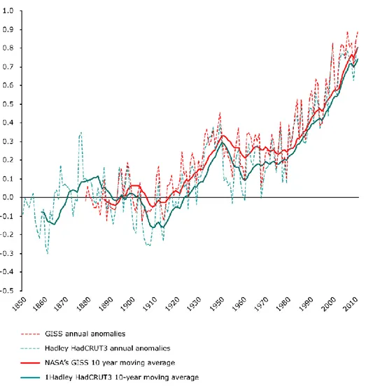
Increasing emissions of greenhouse gases are now widely acknowledged by the scientific community as the major cause of recent increases in global mean temperature (about 0.5 °C since 1970, figure 1.2) and changes in the world‘s hydrological cycle (IPCC, 2007), including a widening of the Earth‘s tropical belt (Seidel et al., 2008; Lu et al., 2009).

Figure 1.2. Observed global annual average temperature deviations in the period 1850–2010 (in ºC). Different lines refer to different models and databases (available online from http://www.eea.europa.eu/data-and-maps/indicators/global-and-european-temperature/global-and-european-temperature-assessment-4)

(15)

10

Even under conservative scenarios, future climate changes are likely to include further increases in mean temperature (about 2–4 °C globally) with significant drying in some regions (Christensen et al., 2007; Seager et al., 2007), as well as increases in frequency and severity of extreme droughts, hot extremes, and heat waves (IPCC, 2007; Sterl et al., 2008).

As the European Environmental Agency reports, briefly but still concisely,

―The global average temperature is projected to continue to increase. Globally, the

projected increase in this century is between 1.8 and 4.0 0C (best estimate), and is considered likely (66 % probability) to be between 1.1 and 6.4 0C for the six IPCC SRES scenarios and multiple climate models (IPCC, 2007a), comparing the 2080 - 2100 average with the 1961 - 1990 average. These scenarios assume that no additional policies to limit greenhouse gas emissions are implemented (IPCC, 2007). The range results from the uncertainties in future socio-economic development and in climate models. The EU and UNFCCC Copenhagen Accord target of limiting global average warming to not more than 2.0 0C above pre - industrial levels is projected to be exceeded between 2040 and 2060, for all six IPCC scenarios”

1.3.2 Climate change on Mediterranean basin

The Mediterranean basin is characterized by mild, rainy winters and hot, dry summers. The climate is affected by complex interactions between mid-latitude and tropical processes that, overall, make the Mediterranean a potentially vulnerable region to climatic changes as induced, for example, by increasing concentrations of greenhouse gases (Giorgi and Lionello, 2008; Ulbrich et al., 2006).

Indeed, the Mediterranean region has shown large climate shifts in the past (Luterbacher et al., 2006) and it has been identified as one of the most prominent hot-spots in future climate change projections (Giorgi and Lionello, 2008).

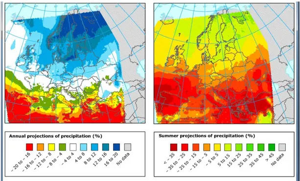
Giorgi and Lionello (2008) have presented a review of climate change projections over the Mediterranean region based on the latest and most advanced sets of global and regional climate model simulations. These simulations have given a collective picture of a substantial drying and warming of the Mediterranean region, especially in the warm season (precipitation decrease exceeding −25–30% and warming exceeding 4–5 °C). These signals are visible in most projections from both Global and Regional Climate Models (RCMs) (CIRCE; Van Der Linden, 2009; Ulbrich et

(16)

11

al., 2006), and although there are considerable uncertainties in climate model predictions, they agree that more frequent and intense droughts are expected (figure 1.3).

Looking for more specific climate projections for the Mediterranean , CIRCE project argues that temperature would increase of 2-4°C while a decrease of precipitation of 5-10% is expected in the next 40‘s years, projections that overall are consistent with those reported by the European Environmental Agency (figure 1.3)

Figure 1.3. Projected changes in % in annual and summer precipitation between 1961–1990 and 2071–2100 as simulated by ENSEMBLES Regional Climate Models for the IPCC SRES A1B emission scenario.

1.3.3 Expected consequences of Climate Change on forest system

Forested ecosystems are being rapidly and directly transformed by the land uses of our expanding human populations and economies. Currently less evident are the impacts of ongoing climate change on the world‘s forests. Understanding and predicting the consequences of these climatic changes on ecosystems is emerging as one of the grand challenges for global change scientists, and forecasting the impacts on forests is of particular importance (Boisvenue and Running, 2006; Bonan, 2008). Forests, here broadly defined to include woodlands and savannas, cover 30% of the

(17)

12

world‘s land surface (FAO, 2006). Around the globe societies rely on forests for essential services such as timber and watershed protection, and less tangible but equally important recreational, aesthetic, and spiritual benefits. The effects of climate change on forests include both positive (e.g. increases in forest vigour and growth from CO2fertilization, increased water use efficiency, and longer growing seasons)

and negative effects (e.g. reduced growth and increases in stress and mortality due to the combined impacts of climate change and climate-driven changes in the dynamics of forest insects and pathogens) (Ayres and Lombardero, 2000; Bachelet et al., 2003; Lucht et al., 2006; Scholze et al., 2006; Lloyd and Bunn, 2007).

Considerable uncertainty remains in modeling how global climate change will affect the risk of future tree die-off events, referred to hereafter as ‗forest mortality‘, under a changing climate (Loehle and LeBlanc, 1996; Hanson and Weltzin, 2000; Bugmann et al., 2001). Although a range of responses can and should be expected, recent cases of increased tree mortality and die-offs triggered by drought and/or high temperatures raise the possibility that amplified forest mortality may already be occurring in some locations in response to global climate change. Examples of recent die-offs are particularly well documented for southern parts of Europe (Penǖelas et al., 2001; Breda et al., 2006; Bigler et al., 2006) and for temperate and boreal forests of western North America, where background mortality rates have increased rapidly in recent decades (Van Mantgem et al., 2009) and widespread death of many tree species in multiple forest types has affected well over 10million ha since 1997 (Raffa et al., 2008). The common implicated causal factor in these examples is elevated temperatures and/or water stress, raising the possibility that the world‘s forests are increasingly responding to ongoing warming and drying.

(18)

13

1.4 Wetlands and Water Resource

Water availability is considered the environmental factor that most strongly limits plant growth world-wide (Nemani et al., 2003). Global change is expected to exacerbate alterations in the world's hydrological cycle (IPCC, 2007). An overall decrease in soil moisture is already underway (Jung et al., 2011).

The UN Millennium Ecosystem Assessment (2005) determined that environmental degradation is more prominent for wetland environments than for any other ecosystem on Earth. International conservation efforts and the development of rapid assessment tools are being used in conjunction with each other to inform people about wetland issues (MEA, 2005). Wetlands are among the most species-rich environments known (Ward et al. 1999; Mitsch et., 2007). They may often be described as ecotones providing a transition between water bodies and arid or semi-arid regions. Many of the flora and fauna that are part of wetlands are disappearing. As most species are endemic of wetlands, biologists and other scientists routinely census wetland biota to look for threatened populations. The IUCN's global red list (online available at www.iucn.org) can be accessed on the internet to determine if there is any species within a particular wetland system that has been identified as needing assistance to prevent extinction.

The Mediterranean basin, characterized by mild, rainy winters and hot, dry summers, supports characteristic Mediterranean forests, woodlands, and scrub vegetation. Nevertheless, the Mediterranean has a very large number of wetlands, for a total of over 8 million and a half hectares.

The Mediterranean Wetlands Observatory (2011) presents the results of a three- year project on Mediterranean wetlands studies in which seventeen indicators have been developed and evaluated. The results of these analyzes suggest: contrasting trends for wetlands biodiversity between the Western and the Eastern Mediterranean regions; very strong and growing pressure on water resources and multiple causes of degradation on wetlands; Political and governance issues in addition to the institutional divides between main stakeholders are the main causes of these pressures.

(19)

14

1.4.1 Mediterranean Plain Oak Forests of Central Italy

The vegetation in Mediterranean climates is typically sclerophyllous and ever-green, adapted to water stress during the dry summer period, and able to grow on infertile soils (Gasith andVincent, 1999) . The availability of year-round moisture near streams enables deciduous woody vegetation to occur in the riparian zone as seen in Mediterranean-type streams in the Northern Hemisphere (Holstein, 1994) with equivalent species pairs occurring in different Mediterranean regions (e.g. Israel and California).

Coastal plain forests of the Tyrrhenian, thermophiles and sub-acidophilic, have settled on the morphology of coastal plain with shallow groundwater and alluvial substrates such as the ancient Pleistocene dunes, flattened and pedogenesized. In the past, hygrophilous and meso-hygrophilous woods behind the dunes and interdunal wet environments, had a wide distribution along the Italian coast. The works of land reclamation and deforestation in the sub-coastal plain area of Lazio were made mostly between 1926 and 1936. During the clean most of the interdunal depressions were filled with sediment and channels were built to drain the deepest. Nevertheless, in the woods wrecks left, located above the Pleistocene dune complex, some small depressions, namely vernal pools (figure 1.4), have survived and others have been restored. Within these, water accumulates for several months a year. In these pools the water table once emerged on the surface during the rainy periods, but today is a much deeper level.

Figure 1.4 A typical vernal pool in Circeo National Park

The gradual lowering of water table, because of drainage and water collection, has attracted scientific interest on the possible evolution of these environments,

(20)

15

particularly in relation to seasonal variations, climatic and succession changes (Stanisci et al, 1998).

Currently, plain forest are scarce and localized, due to strong anthropogenic changes (sewage, drainage, cultivation, construction, tourism). However, in the Tyrrhenian coast of Tuscany and Lazio (Italy) we can still find some rare examples of this type of vegetation, fairly well conserved (Stanisci et al, 1998).

The high availability of edaphic water allows the coexistence of sclerophyllous evergreen oak species (Q. ilex and Q. suber) with deciduous ones (dominated by a typical endemism of Q. cerris and Q. frainetto and with the significant presence of

Q. robur) despite the meso-Mediterranean or thermo-Mediterranean climate location

(Presti et al., 1998).

Despite the ecological value of these forests due to the high biodiversity, micro-heterogeneity and their present reduced extension, few scientific concern has been directed towards these forest complex and their existence is not even mentioned in recent reviews of wetlands. currently they have not ever been included in Europe's most threatened natural ecosystems and are not listed in Annexe I of the European Habitats Directive as being a 'priority forest habitat type'.

Model testing of the present study was carried out at the protected plain forest of Castelporziano Estate (CPE), mainly covered by holm-oak (Figure 1.4). Some information about the plain forest of Circeo National Park (CNP), mainly covered by turkey oak, have been integrated.

(21)

16

1.4.1a Castelporziano Estate (CPE)

The Presidential Estate of Castelporziano, located about 20 km from Rome (41°44′N, 12°25′E), covers an area of 6100 ha (Figure 1.5). This area is fairly flat, ranging from sea level to 85 m a.s.l.

The climate is of Lower Mesomediterranean Thermotype, Upper Arid/Lower Subhumid Ombrotype (Blasi, 1994).

The holm-oak wood of Castelporziano (about 100 ha) is a rare example of holm-oak forest belonging to the Viburno-Quercetum ilicis (Br.-Bl. 1936) Rivas-Martinez (1975) association. This association is the warmest and most thermophilous type of such woods in Italy, formed in a coastal environment on consolidated dunes and on the sea-facing slopes, in a definitely Mediterranean environment (Pignatti, 1998). The soil consists of reddish, quartziferous aeolian sands of the ancient dunes (Manes et al ., 1997c).

(22)

17

1.4.1b Circeo National Park (CNP)

The Circeo National Park, located about 100 km south of Rome, extends from latitude 41°13′N to 41°24′N, and from longitude 12°50′E to 13°07′E (Fig. 1.4). This is a coastal area with a climate of Lower Mesomediterranean Thermotype, Upper Subhumid Ombrotype (Blasi, 1994). In 1977 the Park was included in the network of Biosphere Reserves of UNESCO‘s MAB Programme.

Also present are coastal lakes and wetlands, seasonally flooded, which have been declared ‗Wetlands of International Interest‘ according to the Ramsar Convention. The Circeo National Park (about 8400 ha) consists of five main environments: the plain forest, four coastal lakes, the coastal dune area, the limestone massif of Mount Circeo, with a maximum height of 541 m a.s.l., and the island of Zannone. The plain forest covers about 3190 hectares and consists mainly of deciduous woods ( Q. cerris L., Q. Frainetto Ten., Q. Robur L., Fraxinus ornus L. And Carpinus betulus L.), with soils that are mainly characterized by Würmian sand with pyroclastic material, referred to as the Vulcano Laziale activity (Manes et al ., 1997a; Dowgiallo & Bottini, 1998). The forest is of relatively mesophytic mixed broad-leaved oaks belonging to the Teucrio siculi-Quercion cerridis (Ubaldi, 1988) Scoppola et Filesi 1993 alliance (figure 1.6), which is well represented in Italy.

(23)

18

Figure 1.6. Three typical vegetation profile of Circeo National Park plain forest. Arciglioni: contact between the Holm oak and Turkey oak with Hungarian oak (A), the forest of Holm oak and Cork oak (B) and Alders (C); Selvapiana: Hungarian oak wood and Cork in its typical aspect (A) and in the mesophyll with English oak and laurel into bay depressions (B) Cerasella: contact of Turkey oak and Hornbeam with Hungarian oak (A) and the forest with English oak and Ash of the pools (B); (modified by Presti at al., 1998)

(24)

19

1.5 Theoretical Framework

1.5.1 Why a Dynamical Systems Theory

Models provide a much more powerful tool than qualitative reasoning for showing that certain mechanisms can lead to phenomena of interest such as regime shift (Scheffer and Carpenter, 2003).

Although dynamic models are used for many purpose, we can put them under two broad headings: theoretical understanding of how the system operates, and practical

applications where model predictions will play a role in deciding between different

possible courses of action (Table 1.2). It is important to keep in mind this distinction because it affects how we build and evaluate models.

A theoretical model has to be simple enough that we can understand why it is doing what it does. The relationship between hypotheses (model assumptions) and conclusions (properties of model solutions) is what provides understanding of the biological system. Replacing a complex system that we don‘t understand with a complex model that we also don‘t understand has not increased our understanding of the system.

(25)

20

Most models in the literature are so-called minimal models because focus on a minimal set of mechanisms needed to produce a certain behaviour. A drawback of simple models is that they necessarily leave out many potentially important aspects. However such models have been useful for exploring mechanisms that are too intricate to grasp from common sense alone (Scheffer and Carpenter, 2003).

Theoretical models are well suited to describe complex ecosystem that are characterized by historical dependency, nonlinear dynamics, threshold effects, multiple basins of attraction, and limited predictability (Levin, 1999). Biological processes are typically characterized by nonlinear relationships and feedback process that often result in unpredictable phenomena.

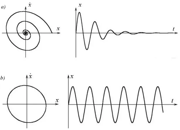
Many parts dynamical systems theory deal with asymptotic properties of systems behavior, i.e., what happens with the system after a long period of time. Here, the focus is not on finding exact solutions to the equations defining the dynamical system (which is often hopeless), but rather to answer questions like "Will the system settle down to a steady state in the long term, and if so, what are the possible steady states?", or "Does the long-term behaviour of the system depend on its initial condition?". The knowledge of the set of all possible solutions which satisfy the system is not strictly necessary in order to understand the dynamics of a systems. First because it is possible to calculate approximate solutions with a numerical method. Second, because the understanding of the system behaviour is obtained by exploring the structure, or qualitative proprieties, of the invariant phase space, whose simply represents the curves of the unique solutions (trajectories) for different initial conditions. The simplest structure are exhibited by equilibrium points (or

fixed points) and by periodic orbits (Figure 1.7)

The question arises if such characteristic structures are stable and under which conditions the stability is preserved, where the concept of stability means that the trajectories do not change too much under small perturbations of initial conditions. Various criteria have been developed to prove stability or instability of an structure. Under favourable circumstances, the question may be reduced to a well-studied problem involving eigenvalues of matrices. A more general method involves Lyapunov functions. For a more general survey on dynamical systems theory, see Strogatz (1994) and Kuznetsov (2004).

(26)

21

Figure 1.7. Visualisation of simplest dynamical systems structures. a) time series of free oscillations for a linear damped model (right side) and the same time series projected into the phase space (left side). We can see a fixed point like an attractor in the phase space. b) Time series of linear harmonically loaded system (right side) and the same time series projected into the phase space (left side).

1.5.2 Mathematical formalization

A dynamic model is a mathematical formalization describing the evolution of the state of one or more variables. In deterministic model, the variables must be able to uniquely describe the system. Such as variables are called State Variables. A dynamical system consists of three ingredients, namely,

 Time,  State space,  Law of evolution.

When the law of evolution does not depend explicitly on the independent variable t, the system is called autonomous.

a)

(27)

22

The evolution of the state variables can often be well represented by a system of a few ordinary differential equations (ODEs), e.g., matrix or differential equations. This makes them suitable for any type of study whose different components interact in a nonlinear way.

Generally, such a classic deterministic scenario may be written as:

(1)

(2)

where is the vector of state variables, is the vector field defining the law of evolution of the system and is the set of initial conditions from which the system evolves. See Strogatz (1994) for a more detailed description.

The integration of differential equations is possible only for very simple systems. However, an important goal for the dynamic system theory is to describe the solutions at the equilibrium states, like fixed points and periodic orbits, because of they represent the points where the system converges over time. Therefore, I underline what mentioned in the previous paragraph yet: the knowledge of all possible solutions which satisfy the system is not strictly necessary in order to understand the behaviour of a systems.

The solutions at the equilibrium states ( ) can be calculated directly by setting . At equilibrium points, the system is at rest and equilibrium solutions are constant solutions.

Every equilibrium solutions, together with their proprieties, as being attractive or

repellent, stable or unstable, could be affected by disturbances, so that, theoretically,

the equilibrium point would remain the same forever, but in practice there is rarely such a thing as exactness. Due to perturbation in x of f, the location of the equilibrium varies slightly. So the question is how equilibrium solutions of the initial value problem (1-2) behave under the effect of one or more disturbances.

(28)

23

1.5.3 Linear stability analysis

A stationary solution x*is linearly asymptotically stable if the response to a small perturbation approaches zero as the time approaches infinity. A linearly asymptotically stable equilibrium is also called sink and is an example of an

attractor.

A stationary solution x* is stable if the response to a small perturbation remains small as the time approaches infinity.

Otherwise the stationary solution is called unstable and the deviation grows.

It is crucial to realize that the above definitions of stability are local in nature. An equilibrium may be stable for a small perturbation but unstable for a large perturbation.

The behaviour of the system near an equilibrium state is described by the local

stability analysis which can be determined by means of a standard mathematical

method (Ellner and Guckenheimer, 2006)

Briefly speaking the equations describing the model are first linearly expanded around the equilibrium point by a Taylor series expansion.

For more than one state variables, this system of equations is easily written down using the notation of the Jacobian matrix J of the first-order partial derivatives. Evaluated at the equilibrium, the Jacobian is

Now the linearized system in vector notation reads

(29)

24

Consider the linear system , with equilibrium . In the one-variable case we get exponential solutions, . In the multivariable case, we get something similar from the eigenvectors and eigenvalues of the matrix .

Recalling the definition: is an eigenvalue of , and a corresponding

eigenvector, if J (Ellner and Guckenheimer, 2006).

It is important to note that eigenvectors are only defined up to constant: if ωis an eigenvector for J so is for any constant . The requirement that  is important. Without it any number would be an ―eigenvalue‖ corresponding to , because .

Eigenvalues are important because they may give exponentially growing or decaying solutions if they are real numbers, or oscillatory behaviour if they are complex numbers.

This can be demonstrated by direct substitution:

The typical situation for a matrix , that also admits complex eigenvalues, of size is that it will have distinct eigenvalues and corresponding eigenvectors. Then the general solution of is:

As said before, because of the eigenvalues may be complex number, this exponential notation may be include pure exponential terms as well as oscillating terms.

For the stability of a fixed point only one term in (6) really matters: local stability of a fixed point for a system of differential equations depends on the eigenvalue of the Jacobian matrix with largest real part (Ellner and Guckenheimer, 2006) They may be evaluated simply by finding the roots of the characteristic equation

(30)

25 Where I is the identity matrix.

The stability of a fixed point may be:

 Stable if all eigenvalues of the Jacobian have negative real part.  Unstable if any eigenvalue of the Jacobian has positive real part.

 If the real part of any eigenvalue is exactly 0, the equilibrium may either be stable or unstable – local linearization is inconclusive.

A more comprehensive discussion of the topic can be found in Ellner and Guckenheimer (2006) and Kuznetsov (2004).

A stable fixed point may be attractive, meaning that if the system starts out in a nearby state, it will converge towards the fixed point. Similarly, one is interested in

periodic points, states of the system which repeat themselves after several time steps.

Even simple nonlinear dynamical systems often exhibit almost random, completely unpredictable behaviour that has been called chaos.

Behaviour and fixed point can be observed in a phase space, that is a Cartesian representation whose axes are of state variables and whose each possible state of the system corresponding to one unique point in the phase space (see 1.7)

When two different phase portraits represent the same qualitative dynamic behaviour (i.e. a single attractor, limit cycle etc.) the behaviour of different systems are defined as topological equivalent. The set of initial conditions that lead to the same final system behaviour define the attraction basin, that is the ecological resilience.

1.5.4. Bifurcation

The parameter change may causes the stability of an structure to change. In particular, fixed points can be created or destroyed, or their stability can change. This qualitative change in the dynamics are called Bifurcations, and the parameters values at which they occur are called Bifurcation Points. Bifurcations are important scientifically because of they provide models of transitions and instabilities as some

control parameters are varied.

In continuous systems, this corresponds to the real part of an eigenvalue of an equilibrium passing through zero. Bifurcations occur in both continuous systems

(31)

26

(described by ODEs, DDEs or PDEs), and discrete systems (described by maps). Bifurcation may be:

 Local, which can be analysed entirely through changes in the local stability properties of equilibria, periodic orbits or other invariant sets as parameters cross through critical thresholds;

 Global, which often occur when larger invariant sets of the system 'collide' with each other, or with equilibria of the system. They cannot be detected purely by a stability analysis of the equilibria (fixed points).

Now I introduce the simplex types of bifurcations to which it is possible to link the majority of cases with only one control parameter.

1.6.4a Saddle-node Bifurcation

In the mathematical area of bifurcation theory a saddle-node bifurcation, tangential

bifurcation or fold bifurcation is a local bifurcation in which two fixed points (or

equilibria) of a dynamical system collide and annihilate each other. The term

saddle-node bifurcation is most often used in reference to continuous dynamical systems. In

discrete dynamical systems, the same bifurcation is often instead called a fold bifurcation. Another name is blue skies bifurcation in reference to the sudden creation of two fixed points.

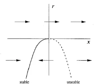
The prototypical example of a saddle-node bifurcation is given by the first-order system

Where r is a parameter, which may be positive, negative, or zero. When r is negative, there are two fixed points, one stable and one unstable.

As r approaches 0 from below, the parabola moves up and the two fixed points move toward each other. When , the fixed points coalesce into a half-stable fixed point at . This type of fixed point is extremely delicate since it vanishes as soon as and now there are no fixes points at all. In this example, we say that a bifurcation occurred at , since the vector field for and are qualitatively different.

(32)

27

Figure 1.10 Saddle-node bifurcation for eq. (8).

The rationale is that r play the role of an independent variable, and so should be plotted horizontally. The drawback is that now the x-axis has to be plotted vertically, which looks strange at first. Arrows are sometimes included in the picture, but not always. This picture is called bifurcation diagram.

In a certain sense, the prototypical form, or normal forms, are representative of all the same type of bifurcation, like in this case it is representative of the all saddle-node bifurcations. The idea is that, close to a common bifurcation, the dynamics typically look like its normal form.

(33)

28

1.5.4b Transcritical Bifurcation

Mathematically a transcritical bifurcation is a particular kind of local bifurcation, characterized by an equilibrium having an eigenvalue whose real part passes through zero.

In such type of bifurcation a fixed point exists for all values of a parameter and is never destroyed. However, such a fixed point interchanges its stability with another fixed point as the parameter is varied. In other words, both before and after the bifurcation, there is one unstable and one stable fixed point. However, their stability is exchanged when they collide. So the unstable fixed point becomes stable and vice versa.

The normal form of a transcritical bifurcation is

This equation is similar to logistic equation but in this case we allow r and x to be positive or negative (while in the logistic equation x and r must be non-negative). The two fixed points are at and . When the parameter r is negative, the fixed point at is stable and the fixed point is unstable. But for 0, the point at is unstable and the point at is stable. So the bifurcation occurs at .

Figure1.12 shows the vector field as r varies. Note that there is a fixed point at for all values of r.

Figure 1.12 Transcritical bifurcation for eq. (9)

Figure 1.13 shows the bifurcation diagram for the transcritical bifurcation. As in figure ppp the parameter r is regarded as the independent variable, and the fixed points and are shown as dependent variables.

(34)

29

Figure 1.13 Transcritical bifurcation diagram for eq. (9)

1.5.4c Pitchfork Bifurcation

In continuous dynamical systems, pitchfork bifurcations occur generically in systems with symmetry. There are two very different types of pitchfork bifurcation. The simpler type is called supercritical, the other one subcritical.

The normal form of the supercritical pitchfork bifurcation is

This equation is invariant under the change of variables . This invariance is the mathematical expression of the left-right symmetry mentioned earlier. Figure 1.14 shows the vector field for different values of r.

When the origin is the only fixed point, and it is stable. When the origin is still stable, but much more weakly so, since the linearization vanishes. Finally, when the origin has became unstable. Two new stable fixed points appear on either side of the origin, symmetrically located at .

(35)

30

Figure 1.14 supercritical pitchfork bifurcation for eq. (10).

The bifurcation diagram is shown in figure 1.15

Figure 1.15 Supercritical pitchfork diagram for eq. (10).

In a specular way to the previous one, the normal form for the subcritical case is:

And the pitchfork is inverted: in this case, for the equilibrium at is stable, and there are two unstable equilibria at . For the equilibrium at is unstable. It is important to note that the origin is stable for and unstable for , as in the supercritical case, but now the instability for is not opposed by the cubic term. The cubic term lends an helping hand in driving the trajectories out to infinity.

(36)

31

(37)

32

2. METHODS

In this chapter I will derive a simple competition model to describe wet forests dynamics. The model includes three state variables, the mass density of the hygrophilous species X (kg m-2), the mass density of the non-hygrophilous ones Y

(kg m-2) and the soil water content in the rooting zone W (kg m-2 or mm).

The model is spatially implicit this, means that densities are averaged over space, spatial anomalies are not considered and that populations are well-mixed.

2.1 The Model

Growth and functional response of plants to resource availability are generally regarded as the minimum set of factors that should be accounted for in order to explain the observed coexistence of different plant types in forested wetlands (Rodriguez Gonzalez et al., 2010). An abstract dynamic model may therefore take the following form:

(12)

(13)

(14)

where X and Y are the biomass densities (Kg m-2) of, respectively, the hygrophilous

and non-hygrophilous species; W is the soil water concentration (Kg m-2); the

water-dependent functions F and H are net growth rates (yr-1) of the hygrophilous and

non-hygrophilous species; the term k(X+Y) is the death rate (yr-1) due to competition

for space, which is proportional to the total biomass, with constant k (m2 Kg-1 yr-1);

the water-dependent functions TX and TY (yr-1) model the water loss to transpiration per unit biomass; the function S (Kg m-2yr-1) represents the algebraic sum of all

biomass-independent sources and sinks of water (e.g. precipitation, percolation, etc.). It is generally reasonable to assume dS/dW<0 because some sinks (e.g. percolation)

(38)

33

increase their flow rate for increasing soil water content, even if some sources (e.g. precipitation) could be largely independent of it.

This abstract formulation should be thought of as valid within an intermediate range of water concentration. The lower end of this range must be above the permanent wilting point, and the upper end must be below the soil saturation concentration. The model values must also be taken as yearly averages, and are not representative of conditions that may occur for shorter times (such as extreme or anomaly events). Outside the validity range of the model, even if the equations remain mathematically well-posed, other biological and ecological factors, which are neglected here, step into the picture. Therefore the model will not yield believable results in arid or permanently swampy environments.

The hygrophilous species' net growth rate F is assumed to be a growing function of soil water concentration W : it attains its highest value at the upper end of the water concentration interval, and its lowest value at the lower end of the interval. The net growth rate H of the non-hygrophilous species is assumed to be a growing function of W only up to some intermediate value of water concentration. For larger water concentrations it either decreases, or, at least, it doesn't increase as rapidly as F. These assumptions are suggested by the dual role of water as a resource and stress factor. In order to better understand this different water responses it is convenient to express the net growth rates as the sum of two terms, that I shall call growth rates (f,

h) and mortalities (m,n).

The growth rates f and hmodel the metabolic growth processes of plants. They are monotonically growing functions of the soil water content, and saturate at high water levels. An explicit expression for fand hmay be given by Michaelis-Menten functions (also known as Hollings Type I)

(39)

34

where gx and gy are the maximum growth rate, attainable in completely idealized conditions. The coefficient WX and WY are half-saturation constants.

In the introduction we have defined non-hygrophilous species as drought-resistant due to their capability to increase the water use efficiency, i.e. the ratio between plant growth and water lost, as the soil dries. Schulze (2005) reports the metabolic activity of plants in relation with water, his work shows that species which assimilate large quantities of CO2 are less stress tolerant (figure 2.1). In those plants, CO2

assimilation decreases with very little soil drying. In contrast species with low rates of CO2 assimilation usually are able to endure drought stress to a a greater degree.

Therefore, although we expect those coefficients to be numerically close to each other, we may generally assume WX > WY to define a different water range for growth optimality, and gx ≥gy to single out the different maximum assimilation rates.

Figure 2.1 The dependence of CO2 assimilation on soil water content for different functional plant types that are sensitive or resistant to drying. Sensitive types have a much higher rate of CO2 assimilation that resistant types when water is abundant (from Schultze, 2005)

The water-dependent mortality functions m and n have distinct behaviour for the two species. For the hygrophilous species, the scarcity of water is a stress. Therefore we will take m as a monotonically decreasing function of W. For the non-hygrophilous species is the opposite holds: too much water is a stress factor. Therefore we take n

(40)

35

as a monotonically growing function of W . Below we shall use simple rational functions to express mathematically m and n.

Where the coefficients and are expresses in Kg m-2; the coefficients a, c, and b, d (formally the water-induced mortalities of the hygrophilous and non-hygrophilous species, respectively, in the limit ) are in yr-1;

Figure 2.2. summarizes graphically the water-dependent growth and mortality functions of the model. Note that the curves representing the net water-dependent growth rates F and H may or may not meet within the model validity region, depending on the physiological properties of the species being modelled.

Figure 2.2. Water-dependent growth and mortality rates as in equations (1-7). Blue and red lines refer to the hygrophilous and non-hygrophilous species, respectively. The grey shaded area is the validity range of the model. Dashed lines are the growth rates, assumed to be proportional to transpiration; dotted lines are mortalities; solid lines are the resulting net growth rates F(W)=f(W)-m(W) and

H(W)=h(W)-n(W). The parameter values used to draw the figure are: g=0.1 Yr-1, Wx=250 Kg m-2,

Wy=300 Kg m-2 , a=0.02 Yr-1, b=0.075 Yr-1, c=0 Yr-1, d=0.015 Yr-1 , Wθ=90 Kg m-2, W =920 Kg m-2.

Competition for space is modeled by a water-independent death term, proportional to the total biomass. Of course, the last term in equations (12) and (13) disregards

(41)

36

completely a large number of complicated ecologic interactions which may be possible among plants. However, at least as a working hypothesis, it is best to assume that the mere crowding of the forest is the dominant factor affecting the death of trees. Note that, if the water concentration W is externally kept fixed, and one of the two plant species is absent (i.e. Y=0 or X=0 ), the equation for the other reduces to a logistic equation with carrying capacity F(W)/k or H(W)/k . For simplicity, we keep the same coefficient k for both the hygrophilous and the non-hygrophilous species. This choice appears to be appropriate in the case study that we present in section 2.2. If necessary, distinct coefficients may be used, with minimal adjustments to the mathematical analysis presented below.

There is a strong correlation between the growth of plants and their transpiration (Brian and Hicks, 1982) The exact functional form linking the growth rate and the flux of transpired water is unknown, although there is evidence that it changes among different species, at different life stages of the plants, and that it is affected by the local climate (Law et al., 2001, Donovan et al., 1991). However, experimental data for midlatitude forests show that a simple proportionality should be a reasonable approximation (Law et al., 2001; Yu et al., 2008, Brian and Hicks, 1982). Therefore we have, for suitable coefficients, , (dimensionless)

The transpiration rates in response to water variations can be thought of as a necessary cost associated with the metabolic growth. Because of the different strategies for water use efficiency, that cost is not the same for the two species: non-hygrophilous (or drought-resistant) species show lower transpiration rates than hygrophilous species both in drought and in wet conditions. In drought conditions, resistant species are able to control stomata better than sensitive ones: this allows them to achieve relatively high photosynthetic rates with transpiration rates lower than their hygrophilous competitors (Schulze, 2005; Van der Molen et al., 2011; Brian and Hicks, 1982). In the presence of abundant water, hygrophilous species reach photosynthetic rates higher than those of resistant species, but at the expense of higher transpiration rates (Rodriguez Gonzalez et al., 2010; Schulze, 2005; Brian and Hicks, 1982). Therefore we shall assume that .

(42)

37

The only source of water in the model is precipitation, p , assumed to be constant. According to the observational evidence for midlatitude forests (Schulze, 2005; Reichstein et al., 2003), there also exist a non-negligible average evaporation rate e that is independent of plant transpiration. Finally we take the flux of water lost to deep percolation as proportional to the water concentration in the soil, with proportionality constant q. Therefore, the biomass-independent sources and sinks term S assumes the form

With the modelling choices discussed above (4-9), the model equations become

where the parameter‘s definition and units are listed in table 2.1

Parameter or process Description Unit

g Relative growth rate Yr-1

WX, WY Half saturation constant Kgm-2

a, c X and Y‘s mortality in the limit in which W tends to 0 Yr-1 b, d X and Y‘s mortality in the limit in which W tends to ∞ Yr-1

, Coefficients that determine the shape of mortalities curve Kgm-2

k Death rates due to space competition, m2 Kg-1 Yr-1

p Precipitation Kgm-2

α, β X and Y‘s max transpiration rates (dimensionless)

e Soil evaporation Kgm-2

q Average Deep Percolation Kgm-2Yr-1

(43)

38

2.2 Comparison with observations

In order to calibrate the model, I have fitted the parameters with the available experimental data measured at two Mediterranean plain forests of Central Italy (Circeo National Park and Presidential Estate of Castelporziano) assuming, for simplicity, that those ecosystem are at equilibrium state. The goal of this analysis is twofold: on one hand, it shows that the model is able to describe the coexistence of hygrophilous and non-hygrophilous species in a way which is coherent with the observed state of the forest ecosystem; on the other hand, it gives a quantitative tool for assessing the resilience of states of coexistence to climate change.

All parameters have been determined, either directly or indirectly, from available data in literature, referring to year-averaged quantities. Due to the experimental uncertainties, some parameters can only be roughly estimated, while others allow for a precise fit.

However, it should be noted that, generally, the results of a such theoretical model, based on initial qualitatively assumption and with secondary neglected factors, are unlikely to be accuracy comparable with empirical observations. Rather what we expect is a good agreement with the orders of magnitude and the range within which these processes vary for different imposed conditions

2.2.1 Observations on Mediterranean plain forest

Observational data about Mediterranean coastal plain oak forests can be summarized in the following points: (i) deciduous species generally show cavitation at higher soil water content than the evergreen (Tyree and Cochard, 1996) which makes them more vulnerable to drought stress (figure 2.3); (ii) oaks vary their leaf area index, adjust their stomatal openings, and extend their root system to tap groundwater in such a way as to ensure that evaporation is less than the water supply (Baldocchi and Xu, 2007); This will be the reason why climatic change will be introduced in the model by modifying the soil water supply, i.e. changing difference p-e rather than the potential transpiration ratios α and β; (iii) forest conenoses distribution is closely related to micro-geomorphological conditions of soil and water. In these areas the water availability has been identified as the major factor shaping vegetation

(44)

39

distribution and controlling plant functions (Presti et al., 1998; Rambal, 2011). According to what I have shown in section 1.1.1, I define the deciduous species as the Hygrophilous competitors while the evergreen will represent the non-hygrophilous ones. Now let's have a look at a range in the model parameters that enable model to qualitatively reproduce all the three points of section 2.2.

Figure 2.3. Vulnerability curves for six species of oak. X-axis is the xylem pressure potential needed to induce the percent loss hydraulic conductivity on the Y-axis (from Tyree and Cochard, 1996)

2.2.2 Model parameterization

The model has 15 parameters. So it would take at least 15 independent data.

Due to the lack of sufficient data, some parameters were calibrated according to the expected orders of magnitude and according to some assumptions delivered a priori.