Andrea Albarea, Michele
Bernasconi, Cinzia Di Novi,
Anna Marenzi,
Dino Rizzi, and Francesca
Zantomio
Accounting for tax evasion
profiles and tax expenditures in
microsimulation modelling. The
BETAMOD model for personal
income taxes in Italy
ISSN: 1827-3580 No. 24/WP/2015
W o r k i n g P a p e r s D e p a r t m e n t o f E c o n o m i c s C a ’ F o s c a r i U n i v e r s i t y o f V e n i c e N o . 2 4 / W P / 2 0 1 5 I S S N 1827 -3580
Accounting for tax evasion profiles and tax expenditures in
microsimulation modelling. The BETAMOD model for personal
income taxes in Italy
Andrea Albarea, Michele Bernasconi, Cinzia Di Novi, Anna Marenzi, Dino Rizzi, Francesca Zantomio
Department of Economics, Ca’ Foscari University of Venice
July 2015
Abstract
The paper presents the main characteristics of BETAMOD, a static microsimulation model that reproduces the
Italian personal income tax (IRPEF), as well as local income taxes, namely the regional and municipal additional income taxes, building on a detailed reconstruction of tax legislation. With respect to the vast majority of existing tax microsimulation models, the peculiarities of BETAMOD concern two aspects: the inclusion of a detailed set of tax expenditures, and the estimation of individual-specific tax evasion rates, which account for the total individual income level, its composition in terms of income sources, and the geographical area of residence.
KeyWords: Tax-benefit microsimulation, tax evasion, tax expenditures, SILC, Italy JEL Codes: C15, C63, H20, H24, H26, H31
Address for correspondence:
Anna Marenzi Department of Economics Ca’ Foscari University of Venice Cannaregio 873, Fondamenta S.Giobbe 30121 Venezia - Italy Phone: (++39) 041 2349148 Fax: (++39) 041 2349210 E-mail: [email protected]
This Working Paper is published under the auspices of the Department of Economics of the Ca’ Foscari University of Venice. Opinions expressed herein are those of the authors and not those of the Department. The Working Paper series is designed to divulge preliminary or incomplete work, circulated to favour discussion and comments. Citation of this paper should consider its provisional character.
The Working Paper Series is available only on line (http://www.unive.it/nqcontent.cfm?a_id=84917) For editorial correspondence, please contact: [email protected]
Department of Economics Ca’ Foscari University of Venice Cannaregio 873, Fondamenta San Giobbe 30121 Venice Italy
1. INTRODUCTION
The increasing complexity of fiscal challenges requires appropriate instruments to evaluate the revenue effects and the distributional consequences of specific policies. Microsimulation models, based on representative sample of individuals or households, take into account the heterogeneity of individual behavior, reproduce a part or the whole tax and benefit system of a country, regions or group of States (Sutherland and Figari, 2013) and are able to identify the winners and the losers of tax/transfer policies. Microsimulation models have become in many countries a standard tool for the design and the evaluation of public policies (see, among others, Bourguignon and Spadaro, 2006; Mitton, Sutherland and Weeks, 2000).
This paper presents a new microsimulation model, called BETAMOD, for Italian personal income
tax (IRPEF), as well as local income taxes, namely the regional and municipal additional income
taxes.
BETAMOD improves on existing models1 in two ways: first, by estimating a distribution of
individual tax evasion rates, based on total individual income level, its composition in terms of sources, and geographical area; second, by accounting for a detailed set of tax allowances, which are currently the object of fiscal policy reforms debate, at the national and international level (e.g. Tyson, 2014). For different reasons, the two aspects are relevant in the Italian institutional setting and therefore deserve particular attentions.
Tax evasion in Italy is extremely high and various political leaders as well as a significant share of the public opinion seem to justify tax evaders using the argument that the tax rates are too high and the tax schedule too progressive. The answer to the above question depends on the redistributive effects of tax evasion and, more specifically, on the distinct effects that tax evasion may have on progressivity (vertical effect) versus horizontal equity and re-ranking (Aronson and Lambert, 1994). With respect to other Italian models, where tax evasion rates are assumed to be constant within population subgroups (e.g. by income source type, by income classes), BETAMOD, assigns a tax evasion rate to each individual. This allows to evaluate more accurately
how tax evasion may alter the redistributive effect of personal income taxation, and to measure the horizontal, vertical and re-ranking effects, each of which is possibly altered by tax evasion. Over the last decade, tax expenditures in Italy have increased as a share of GDP. The Italian
Ministry of Economy and Finance identifies 720 measures of tax expenditures that, in percent of
1 In the past decade several microsimulation models were developed in Italy. Models belong to the same type of
BETAMOD are: the Siena microsimulation model (SM2) for net-gross conversion of EU-SILC income variables (Betti
et al. 2011); the MAPP model for studying the effects of taxes and transfers (in cash and in kind) on the level of poverty and inequality (Baldini et al., 2011); the TABEITA model that reproduces the Italian personal income tax (Ceriani et. al, 2013), and the microsimulation model developed by Pellegrino et al. (2011) for the analysis of housing taxation.
GDP, account for about 10.66 (MEF, 2011). Among them, the individual income tax expenditures
are the largest (4.84% of GDP). Because of the entailed reduction in tax revenues, and the
induced distortions in taxpayers’ behavior, there is an increasing debate on the use of tax expenditures as alternative to direct expenditures (see, Burman, 2003; Burman et al., 2008; Poterba, 2011). Compared to current microsimulation models for Italy, BETAMOD includes all
kind of individual income tax expenditures and allows us to estimate the distributional effects of all tax expenditures simultaneously and of specific tax reliefs or categories of expenditure.
The paper is organized as follows. Section 2 describes the data set and the preliminary data adjustments and imputations required to simulate accurately the Italian personal income taxes. Section 3 illustrates, in details, the process of constructing BETAMOD, focusing in particular on its
innovative aspects. Section 4 tests the robustness of the model by comparing the baseline simulation of personal income tax and local income taxes with official figures provided by tax returns data. Finally, Section 5 provides novel distributional evidences on tax evasion and on its profile, as well as on individuals’ re-ranking between income classes resulting from it2.
2. THE MICRO DATABASE AND RELATED IMPUTATIONS
BETAMOD runs on the Italian national version of the Survey of Income and Living Conditions
(IT-SILC), which represents, with a few exceptions, the micro-database currently chosen by most
tax-benefit microsimulation models for Italy3. With respect to the alternative Survey on
Households Income and Wealth (SHIW), IT-SILC takes the advantage of a more generous sample
size (19,399 households in IT-SILC versus 7,951 households in SHIW), allowing to conduct
analyses by geographical area sample; the drawback of this choice is the lack of information on household’s assets and tax-relevant expenditures.
We use the cross-sectional component of IT-SILC 2011, which features a considerably larger
sample size than the rotating longitudinal component. The interview is structured into an household level questionnaire, collecting information on household composition, accommodation, housing costs, and economic circumstances (including savings, debts, receipt of family-related and means-tested benefits and children’s incomes); and an individual level questionnaire, which is administered to all household members aged 16 years old or above. In the
2 Further material s provided in three Appendices. Appendix A describes the statistical matching between the IT-SILC
dataset and the Bank of Italy's Survey on Households Income and Wealth (SHIW);Appendix B illustrates the
methodology used for the estimation of individual tax evasion rates, and Appendix C shows the incidence of tax reliefs on reported income.
3 For instance, SM2model (Betti et al., 2011), MAPP model (Baldini et al., 2011), and the EUROMOD module for Italy
(Sutherland and Figari, 2011) use IT-SILC data; while, TABEITA model (Ceriani et al., 2013) and the microsimulation model developed by Pellegrino et al. (2011) considers as input data those provided by the Bank of Italy in the Survey on Households Income and Wealth (SHIW).
individual level questionnaire, besides information on education, health and occupation, detailed information on individual’s income from various sources relevant for tax base assessment (employment, self-employment, old age and disability pensions, incapacity and disability benefits, rents from properties, investment income and other incomes) is covered. For income components subject to taxation4, the amount as net of taxes (and of social insurance
contributions, where applicable) is collected, because net amounts are generally regarded as less exposed to measurement error and recall bias than gross ones. Reflecting the structure of the Italian fiscal system, where incomes earned in the solar year t are taxed in the following (t+1), the reference period in income-related questions is the previous fiscal year, that is 2010. This represents a mismatch with respect to demographic information, which reflects the situation of households at the time when the fieldwork was carried out (i.e. March and April 2011), and which has therefore been brought backward to 2010.
Still, an accurate simulation of Italian personal income tax requires additional information with respect to IT-SILC topics coverage. Most notably, the personal income tax base includes not only
employment and self-employment income, replacement income, profits from non-corporate enterprises and a marginal part of investment income, but also figurative income on immovable properties, valued as cadastral rent5, which is not covered in the survey. Besides, information on
specific items of expenditures (e.g. healthcare, house refurbishments, etc.) that are relevant for specific tax reliefs, are not available in IT-SILC. Missing information has therefore been imputed,
drawing from other population-representative surveys covering the subject domains of interest. We use the 2010 Survey on Households Income and Wealth released by the Bank of Italy (Bank of Italy, 2012), for imputing information on the self-reported asset value6 of the main residence,
and other immovable properties, used to compute cadastral values. Drawing from the same survey, we also impute insurance premiums and house refurbishments expenditures, relevant for the computation of specific, and quantitatively important, tax reliefs . Imputation from SHIW has
been performed using statistical matching techniques, where SHIW individuals have acted as
‘donors’ of the otherwise missing information for IT-SILC observed ‘recipients’. Matching aims at
selecting, for each IT-SILC recipient, the SHIW donor that is closest to observational identity, i.e.
the most similar in terms of characteristics, observed in both surveys that are predictive of the variable to be imputed. The quality of the matching procedure relies crucially on a so-called
4 Non-taxable incomes and benefits are taken from the survey, rather than simulated, in order to obtain the
disposable income measure.
5 While cadastral income on the main residence is de facto exempted from personal income taxation trough a tax
deduction, it is anyway relevant for other components of the tax benefit system, such as the means test for family benefits. For other properties, according to whether they are rented or left unoccupied, the actual rent received or cadastral income are respectively used in tax base assessment.
common support requirement of overlapping in the distribution of predictive characteristics in the
donors’ and recipients’ samples, which has been empirically tested. The matching procedure we have adopted is based on a combination of stratification and Mahalanobis distance nearest neighbor algorithm (Rubin, 1980). Matching has been performed at the household level and with replacement, that is allowing the same SHIW household to act as donor for multiple IT-SILC
households, if deemed as the most adequate, rather than being discarded after having served once as donor. The donors’ and recipients’ samples have been stratified by main residence homeownership, other properties homeownership and geographical area, so that exact matching on these variables is ensured; then, within each stratum, the donor household has been selected based on the Mahalanobis distance metric, measured on other predictive variables. These include equivalent household income, the percentage of household members with more than upper secondary educational qualification, a set of household composition dummies, and the main earner’s employment status. The quality of matching has been gauged by investigating the balance (e.g. in terms of equality in means) in predictive variables between recipients and matched donors, and the procedure adjusted as long as achieved balance was deemed unsatisfactory. More detail on the implementation of the matching-based imputation, and the achieved balance, is reported in Appendix A.
As a result of the matching-based imputation from SHIW data, information on the asset value of
owned properties is integrated into IT-SILC. However, for fiscal purposes, properties are valued
in terms of cadastral rental values. Therefore, we build on existing Land Registry data, which provide information on the distribution of properties values and corresponding cadastral incomes (separately by gender, by age group, by household composition, by marital status, by geographical area and by main residence/secondary property) to derive a measure of cadastral income from the available information on properties asset values, integrated into IT-SILC. For assessing the
cadastral value of the main residence, Land Registry information on the ratio between asset value and cadastral income is first of all expanded, using the RAS methodology7, to obtain marginal
distributions across 300 subgroups, defined in terms of the above mentioned variables. After the IT-SILC sample has been correspondingly stratified, the cadastral value for IT-SILC households is
computed as the ratio between the asset value of the main residence imputed from SHIW, divided
by the corresponding asset-value-to- cadastral-income ratio8, drawn from the expanded Land
7 The RAS algorithm is an iterative proportional fitting procedure that estimates joint distribution of two or more
variables given their marginal distributions. See Bacharach, 1965.
Registry statistics. A similar procedure is followed for imputing the cadastral value of secondary properties, where appropriate9.
As an additional micro-data source, we use the 201310 MULTISCOPO Survey on Health Conditions
and the Use of Health Services, released by the National Statistical Office (ISTAT, 2014), to
impute information on healthcare expenditures, necessary to compute other major tax reliefs, namely those that involve the largest share of taxpayers. The MULTISCOPO survey has been used
to estimate, at the individual level, the conditional probability of incurring in tax-relevant healthcare expenditures, such as specialists visits, drugs purchases, medical tests and treatments, as a function of predictive characteristics observed again both in MULTISCOPO and in IT-SILC.
These include gender, six age groups, self-assessed health, reported chronic conditions, limitations in activities of daily living, geographical regions, marital status, occupation, education, presence of dependent children and household size11.
The estimated parameters have then been used to predict the probability of incurring in health expenditures for individuals observed in the IT-SILC sample, based on their characteristics. As
illustrated in the later section 3.1, the estimated probability of healthcare spending is then flexibly used, together with fiscal data on tax reliefs, to identify beneficiaries of healthcare tax reliefs, and to impute related expenditure amounts.
3. THE CONSTRUCTION OF BETAMOD
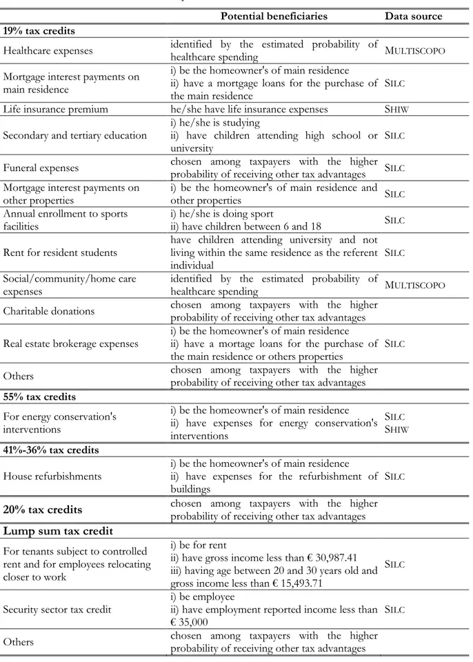
After the preliminary data adjustments and the imputations, the model has been built through 4 modules, integrated in an iterative procedure where outer loops (identifying recipients of tax expenditures, building calibration weights, computing individual- and income-specific tax evasion rates) feed into the inner loop of net-to-gross conversion, as depicted in Figure 1.
In more detail, based on family and personal characteristics relevant for eligibility, Module 1 identifies round-specific beneficiaries and expenditure amounts for all of the non-simulated tax
9 When secondary properties are rented, the actual rent received, as collected in IT-SILC, rather than cadastral
income, enters in the tax base definition.
10 The MULTISCOPO Survey did not take place in 2010. Even though time distance between the interviews in IT-SILC
2010 and MULTISCOPO Survey 2013 seems quite large, this does not constitute an issue since we only used qualitative
information that are actually comparable between the two datasets.
11 We have not included income among the control variables since the MULTISCOPO Survey does not provide any
information about it. However, research findings have suggested that, while at aggregate level there exists a positive and significant relationship between healthcare expenditure and GDP (Newhouse, 1977), at individual level, there is not a significant association between healthcare expenditure and income (especially when the health system provides universal coverage free of charge as the Italian healthcare system does). Indeed, full insurance coverage would remove the individual budget constraint and reduce or eliminate the influence of cost of care on patients’ decisions of how much care to use. Typically, income elasticity of individual healthcare expenditure under full insurance coverage regime tends to be near zero (for details see Getzen, 2000).
reliefs12, calibrating them to obtain the totals and the income distribution for beneficiaries and
expenditures resulting from administrative tax returns data. Module 2 deals with the net-to-gross income conversion, through a standard iterative algorithm. Once gross and reported income measures have been obtained, Module 3 estimates calibration weigths in order to match both population totals and administrative taxpayers counts. By comparison of the grossed-up obtained income measures with disaggregated administrative tax returns data, Module 4 produces an individual tax evasion rate which accounts for the individual’s different income sources composition (employment income, pensions, self-employment income13, rental income from
immovable property), the income level, and geographical residence (North-West, North-East, Center, South). After Module 4, round-specific convergence, measured in terms of equality between reported incomes as estimated by the model14 and as resulting from official tax returns
data15 (both at the aggregate level, and by subgroups defined by main source of income and by
geographical area), is assessed.
The overall iterative procedure, continues until convergence is achieved. Specifically, the iterations stop when the reported levels of income estimated by the model, reflecting estimated tax allowances, tax evasion rates and calibration weights, not differ significantly from official tax returns data, both at the aggregate level and by subgroups (defined by main source of income and geographical area). The overall procedure generates a battery of individual level variables, including true gross income, tax evasion rate, reported income, tax relevant expenditures, calibration weights, for later use in policy simulation modelling. The following sections provide in more detail the four modules and innovative aspects of the model construction.
3.1 Deductions and tax credits module
In the Italian fiscal system there are different kinds of deductions and tax credits. The most sizeable, collectively worth over 5 per cent of GDP, are listed in Table 1, while a comprehensive list of tax reliefs, and their quantitative importance, is reported in Tables 6 and 7.
In terms of design, all deductions and tax credits are non-refundable, with the only exception of the tax credit granted to families with four children. Typically, an upper threshold applies to most
12 A comprehensive list of non-simulated tax reliefs, and of the individual and family characteristics used to identify
the potential beneficiaries is reported in Tables 2 and 3.
13 We consider as self-employed members of the arts and or professions, sole proprietors, free lances, owners or members of a family business and persons receiving profits from non-corporate enterprises.
14 By ‘reported incomes as estimated by the model’ we mean the portion of true gross income that we estimate the
individual will declare, given his tax evasion rate. In what follows, this will be referred to as ‘estimated reported income’, as opposed to ‘reported income’, which refers to official tax returns data.
15 The tax returns of the entire population of taxpayers are disposable on the website of the Italian Revenue Agency
(Ministry of Economy and Finance) only in tabulated form (e.g. by type of income source, by income classes, by area of residence, etc.). Additional ad-hoc data were required for better modelling tax reliefs.
tax expenditures (mortgage interest payments, rent paid by tenants, education), while the healthcare tax credit is allowed on expenses in excess of a lower threshold. Also, a withdrawal rate often applies, so that the fiscal benefit is decreasing in individual’s gross income16.
Figure 1 The construction of BETAMOD
Table 1 The largest PIT deductions and tax credits (fiscal year 2010)
Description (millions of Value
euros)
Percent of GDP
Deductions
Social insurance contributions paid by self-employed individuals 17,603 1.13
Cadastral value of the main residence 8,283 0.53
Voluntary contributions to private pension plans 1,905 0.12
Tax credits
Tax credit for specific income sources 41,887 2.70
Tax credit for dependent family members 11,375 0.73
Tax credit for healthcare expenditures 2,585 0.17
Source: Ministry of Economy and Finance, http://www1.finanze.gov.it/analisi_stat/index.php?tree=2011.
Among deductions, the most relevant in terms of number of recipients and lost revenue, are social insurance contributions paid by self-employed individuals17, the cadastral value of the main
residence and voluntary contributions to private pension plans. Other deductions are granted for specific expenditures, including legal alimony payments to spouses, donations to religious institutions, personal care services and disability aids for the disabled, and social insurance contributions paid for domestic help.
Among tax credits, the largest single item is a universal tax credit granted for specific income sources: the tax credit is applicable for either employment income, or self-employment income, or pension income, with a withdrawal rate resulting in a decreasing credit as gross income increases. This tax credit contribute to the income tax progressivity design, even more so given the absence of a legislated no tax area or legal zero rate tax bracket.
Another set of tax credits aims at accounting for individual’s ability to pay, given her/his household composition (i.e. presence of dependent household members) and her/his children characteristics, such as age and disability. These tax credits are decreasing in individual gross income and become zero above a certain income threshold. The children tax credit amount and income threshold depend also on the number of children, and increase for each child aged three years or below and for disabled children. An additional refundable tax relief is granted for taxpayers with at least four children.
Further tax credits are granted for specific expenditures, and amount to the 19 per cent of such expenditures: these include mainly healthcare, mortgage interest payments on both the main residence and other properties, life insurance premiums, secondary and tertiary education, childcare and charitable donations. Finally, a tax credits for up to a maximum of 55 per cent of the expenses incurred for energy conservation's interventions and house refurbishments, and a lump sum tax credit for rent paid by low-income tenants, are allowed.
As standard in other tax benefit models for the Italian system, and reflecting data availability constraints, BETAMOD fully simulates the deduction for main residence cadastral value, and the
tax credits by income source and for dependent family members18. However, with respect to
existing Italian models, which typically impute tax expenditures though calibration with aggregate fiscal data by income classes, BETAMOD improves by calibrating not only expenditure amounts,
but also beneficiaries. In particular, we aim at achieving a more realistic identification of beneficiaries, for each specific type of tax expenditure item, based on household and personal
17 Employees’ social contributions are not listed among deductions as they are excluded from taxable employment
income.
18 The simulation of tax credit for dependents required the construction of fiscal family that may not coincide with
the definition of household adopted in IT-SILC. In fact, fiscal family members include the spouse, children and other
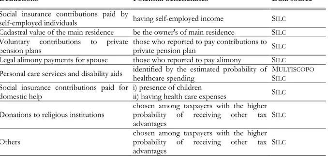
characteristics relevant for eligibility19. Table 2 and Table 3 report the individual and family
characteristics we used to identify the potential beneficiaries of deductions and tax credits.
Simulated and non-simulated tax reliefs include all of the current categories provided by tax rules, namely, 8 deductions and 30 types of tax credits, these last grouped into 16 main categories. Thus, the model offers a complete picture of the wide array of tax reliefs that are part of the Italian income tax.
Table 2 Deductions: identification of potential beneficiaries
Deductions Potential beneficiaries Data source
Social insurance contributions paid by
self-employed individuals having self-employed income SILC Cadastral value of the main residence be the owner's of main residence SILC
Voluntary contributions to private
pension plans those who reported to pay contributions to private pension plan SILC Legal alimony payments for spouse those who reported to pay alimony SILC
Personal care services and disability aids identified by the estimated probability of healthcare spending MSILCULTISCOPO Social insurance contributions paid for
domestic help i) presence of children ii) having health care expenses SILC Donations to religious institutions chosen among taxpayers with the higher probability of receiving other tax
advantages S
ILC
Others chosen among taxpayers with the higher probability of receiving other tax
advantages S
ILC
19 In practice, for certain tax reliefs, due to lack of information in the data, beneficiaries are mainly identified among
the taxpayers with the higher probability of receiving other tax advantage; this is motivated by anecdotal evidence that the probability of claiming specific tax reliefs increases in the number of other tax reliefs claimed. In order to increase variance some beneficiaries have been randomly chosen.
Table 3 Tax credits: identification of potential beneficiaries
Potential beneficiaries Data source 19% tax credits
Healthcare expenses identified by the estimated probability of healthcare spending MULTISCOPO
Mortgage interest payments on main residence
i) be the homeowner's of main residence ii) have a mortgage loans for the purchase of
the main residence S
ILC
Life insurance premium he/she have life insurance expenses SHIW
Secondary and tertiary education i) he/she is studying ii) have children attending high school or
university S
ILC
Funeral expenses chosen among taxpayers with the higher probability of receiving other tax advantages SILC
Mortgage interest payments on
other properties i) be the homeowner's of main residence and other properties SILC Annual enrollment to sports
facilities i) he/she is doing sport ii) have children between 6 and 18 SILC Rent for resident students have children attending university and not living within the same residence as the referent
individual S
ILC
Social/community/home care
expenses identified by the estimated probability of healthcare spending MULTISCOPO Charitable donations chosen among taxpayers with the higher probability of receiving other tax advantages
Real estate brokerage expenses i) be the homeowner's of main residence ii) have a mortage loans for the purchase of the main residence or others properties S
ILC
Others chosen among taxpayers with the higher probability of receiving other tax advantages
55% tax credits
For energy conservation's interventions
i) be the homeowner's of main residence ii) have expenses for energy conservation's interventions
SILC
SHIW
41%-36% tax credits
House refurbishments i) be the homeowner's of main residence ii) have expenses for the refurbishment of
buildings S
ILC
20% tax credits chosen among taxpayers with the higher probability of receiving other tax advantages Lump sum tax credit
For tenants subject to controlled rent and for employees relocating closer to work
i) be for rent
ii) have gross income less than € 30,987.41 iii) having age between 20 and 30 years old and gross income less than € 15,493.71
SILC
Security sector tax credit i) be employee ii) have employment reported income less than
€ 35,000 S
ILC
Once potential beneficiaries have been identified, calibration of amounts and beneficiaries to fiscal data has been carried out for each tax relief type. Calibration accounts not only for income classes, as standard in other experiences, but also, building on the availability of additional ad hoc data obtained from the Ministry of Economy and Finance, for specific relief beneficiaries distribution across occupational status (employee, self-employed and pensioner) and number of dependent household members (none, one, two or more).
Overall, in the light of the importance of tax expenditures in current and future tax reform discussion (Burman, 2003 and 2008, MEF, 2011, Poterba, 2011, Tyson, 2014), BETAMOD can be
used to estimate more accurately the revenue and distributional effects of all tax expenditures simultaneously and of specific tax reliefs or categories of expenditure.
3.2 Gross to net conversion module
To derive gross incomes, we follow a widely used procedure based on an iterative algorithm (see, for instance, Immervoll and O’Donoghue, 2001), represented in Figure 2.
For each taxpayer the procedure estimates an initial true gross income based on an average tax rate applied to net income as collected in the survey, then applies an individual tax evasion rate, and then simulates the appropriate 2010 tax rules to produce a net income measure20, to be
compared with the IT-SILC one.
If they differ, a new estimate of the true gross income is computed applying a correction factor, equal to the ratio between the original and the estimated net income, to the previous round true gross income and a new iteration is run. When equality between the two values is achieved (up to 1 euro of difference), the iteration ends and the data are sent to Module 3 for the reweighting procedure. The output for each individual, feeding into the following modules, includes true gross income, tax evasion rate, estimated reported income, deductions and tax credits, and gross and net income tax liability.
20 In computing individual tax liabilities, deductions are subtracted from reported income, to obtain taxable. The
gross tax is calculated applying the tax schedule to taxable income. Then net tax is obtained subtracting tax credits from gross tax.
Figure 2 Net-to- gross conversion (Module 2)
3.3 Reweighting module
Calibration weighting is a general technique for adjusting probability-sampling weights as of IT
-SILC so that model estimates are consistent with external official data sources (among others, see
Atkinson et al., 1988; D’Amuri and Fiorio, 2006). As external data sources, we consider both population counts (from ISTAT official statistics) and official fiscal data (MEF).
While IT-SILC weights are built to match population totals (ISTAT), we adjust them to achieve
consistency with fiscal data as well, so that the model estimates are reconciled with both the entire population and taxpayers counts. The variables used for performing the individual level
grossing-up are reported in Table 4. In addition to the standard socio-demographic variables, we also consider the number of taxpayers with dependent family members because of the important discrepancies between the sample distribution of household composition and official tax returns data. We obtain the joint distribution across those variables using the marginal distributions in a RAS-like iterative proportional fitting. The household weights are then computed by averaging individual household members weights21. As apparent in the last colum of Table 4, the achieved
difference between BETAMOD recalibrated weights and external official data totals are appealing
with respect to model estimates representativeness.
Table 4 The grossing-up results
Variable Iweight T-SILC Official tax returns BETAMODweight Difference
Total Population 60,683,909 - 60,683,909 0 Males 29,499,829 - 29,499,827 -2 Females 31,184,080 - 31,184,081 1 North West 16,131,196 - 16,131,196 0 North East 11,647,123 - 11,647,123 0 Center 11,943,354 - 11,943,354 0 South 20,962,237 - 20,962,237 0 Age 0 - 14 8,841,850 - 8,841,850 0 Age 15 - 24 6,041,469 - 6,041,468 -1 Age 25 - 44 17,172,717 - 17,172,717 0 Age 45 - 64 16,394,019 - 16,394,019 0 Age over 65 12,233,854 - 12,233,855 1 Total households 25,217,462 - 25,217,462 0 North West 7,186,593 - 7,186,593 0 North East 4,993,636 - 4,993,636 0 Center 5,007,637 - 5,007,637 0 South 8,029,596 - 8,029,596 0 Total Taxpayers - 41,168,189 41,168,317 128 Males - 21,622,165 21,622,249 84 Females - 19,546,024 19,546,068 44 North West - 11,653,491 11,653,533 42 North East - 8,710,500 8,710,532 32 Center - 8,317,613 8,317,638 25 South - 12,486,585 12,486,613 28
Reported income classes
1st quintile - 8,359,593 8,357,026 -2,567
2nd quintile - 7,753,926 7,754,008 82
3rd quintile - 10,526,834 10,527,087 253
4th quintile - 7,851,917 7,852,371 454
5th quintile - 6,675,919 6,677,825 1,906
Taxpayers by main income
Employment income - 20,228,316 20,228,944 628
Pensions - 14,165,864 14,166,862 998
Self-employment income - 2,065,737 4,706,768 -1,504
Rental income from immovable property - 4,708,272 2,065,744 7
Number of taxpayers with dependent
family members - 12,624,414 12624454 40
3.4 The tax evasion module
According to the previous empirical literature concerning tax evasion at micro-level in Italy (Bernasconi and Marenzi, 1997; Florio and D’Amuri, 2006), we apply the “discrepancy method” to estimate tax evasion rates. The method, based on the assumption that individuals report a more truthful income to an anonymous interview than to fiscal authorities, computes tax evasion by comparing the tax returns and income survey responses of similar individuals.
In the above mentioned studies the comparison is made in terms of after-tax income. This choice has two main drawbacks. Firstly, it overestimate the tax evasion rates since it computes them as the ratio of evaded income on net income, instead of on true gross income. Secondly, when taxpayers are compared by quantiles of net incomes, a problem of re-ranking may arise. In fact, with respect to the distribution of after-tax income recorded in the survey, tax evasion shifts downwards individuals in the distribution of net income in the official data, so that, especially at low-income classes, the tax evasion rates are over-estimated. To overcome these drawbacks, BETAMOD estimates tax evasion rates as the percentage differences between the true gross
incomes (as resulting from the net-to-gross conversion module) and the reported incomes declared to fiscal authorities. Clearly, since the true gross income is unknown and it is the results of the net-to gross procedure, tax evasion may be affected by approximations that depends on the estimation method.
Tax evasion rates are estimated in three steps (see Appendix B). In the first step, aggregate tax evasion rates, stratified by area and main income source type, are computed comparing simulated true gross incomes with administrative tax data on reported income. As administrative data are provided in aggregates, by main income source type and, separately, by geographical area, we first apply a RAS technique to obtain the joint distribution of reported income by both dimensions. As a result, a 4×4 matrix of average evasion rates, by income type and geographical area, is obtained (see Table 9).
In the second step a distributional income profile of tax evasion is estimated for each area-by-income type stratum. We refine stratification expanding the 16 strata to account for the profile of tax evasion by income classes. In more detail, each area-by-income type stratum is expanded into 13 classes of true gross income, so that 16 income profiles of tax evasion are obtained. The design of each evasion-by-income profile results from an optimizing procedure, which aims at minimizing the distance between simulated and administrative reported income. The result is a 16×13 dimension matrix of tax evasion rates by main income source type, geographical area and true gross income level.
Finally, a tax evasion rate is assigned to each individual for each type of income source to overcome the standard procedure of assigning the same tax evasion rate to all individuals in each matrix cell. BETAMOD selects randomly, within each cell, individuals to be identified as tax
compliers, and those to be identified as tax evaders, then assigns individual tax evasion rates by using a beta distribution whose mean value is equal to the average tax evasion rate of the cell. Namely, individual tax evasion rates are calibrated so that the sum of individual evaded incomes is equal to the total income evaded in the class.
This represents an advancement, with respect to other models, where tax evasion rates are assumed to be constant within population subgroups (e.g. by income source type, by income classes). This feature allows assessing the relevance of re-ranking between tax-payers due to the presence of tax evasion.
4. VALIDATION AND MAIN RESULTS
The ability of BETAMOD to reproduce each measure (gross income, taxable income, deductions,
tax credits and net tax liability) relevant for personal income tax and local income taxes is validated through a comparison with official figures provided by tax returns data for the relevant fiscal year, that is 2010.
To do this, we first compare the aggregate tax figures simulated by BETAMOD with the official
fiscal statistics. Results are shown in Tables 5, 6 and 7. First, it should be noted that tax evasion reduces the true gross income of about 61 billions of euro, corresponding to an average tax evasion rate of 7.2 per cent (see Table 9). The estimated tax evasion rate might seem relatively low in a country, like Italy, where tax evasion is a widespread phenomenon (among others, Marino and Zizza, 2012; Fiorio and D’Amuri, 2006 and Murphy, 2012). However, the figure reflects the fact that employment income and pensions taken as a whole account for more than the 80% of total reported income (53% and 29%, respectively) and that the estimated average tax evasion rates for these two types of income are, respectively, 2.9 per cent and zero.
As apparent in Table 5, BETAMOD output and official fiscal data presents trivial (i.e. lower than
1%) differences in most figures achieving a very good performance in simulating revenues amounts and taxpayers’ counts22.
The largest difference arises in the number of individuals with positive gross tax liability. This seems mostly driven by the model imputation of tax deductions, resulting in a larger number of individuals with positive taxable income in BETAMOD. This is because tax deductions have been
imputed as a percentage of reported income, thus constraining their amount to be lower than reported income, and therefore taxable income to be positive, by construction.
Focussing on deductions, Table 6 reports the number and the amount of beneficiaries for each type.
Table 5 Aggregate validation: main components of personal income tax and local taxes
Number of taxpayers1 Value2
Totals BETA
-MOD
Official
tax returns Diff % BMODETA
-Official
tax returns Diff %
True gross income 41,168 - - 853,891 - -
Evaded income 14,778 - - 60,789 - -
Reported gross income 41,168 41,168 0.0 793,102 792,520 0.1
Deductions 13,794 13,374 3.1 21,736 21,746 0.0
Taxable income 41,097 39,894 3.0 763,086 762,185 0.1
Gross tax 41,097 39,078 5.2 205,213 205,613 -0.2
Tax credits 39,977 39,088 2.3 64,604 62,482 3.4
Net tax liability 31,178 30,897 0.9 147,904 149,443 -1.0
Regional income tax 31,035 30,653 1.2 8,655 8,633 0.3
Municipal income tax 25,251 25,265 -0.1 3,023 3,021 0.1
Notes: 1 thousands of persons - 2 millions of euros.
Table 6 Aggregate validation: deductions
Number of taxpayers1 Value2
Deductions BETA -MOD Official tax returns Diff % BETA -MOD Official tax returns Diff %
Social insurance contributions paid
by self-employed individuals 11,922 11,991 -0.6 17,601 17,603 0.0 Cadastral value of the main
residence 16,873 17,166 -1.7 8,279 8,283 0.0
Voluntary contributions to private
pension plans 803 822 -2.3 1,897 1,905 -0.4
Legal alimony payments for
spouse 109 120 -9.5 742 745 -0.4
Personal care services and
disability aids 147 143 2.8 537 531 1.2
Social insurance contributions paid
for domestic help 522 537 -2.8 415 419 -0.9
Donations to religious institutions 95 104 -8.7 27 27 -1.8
Others 1,800 1,816 -0.9 517 516 0.1
Notes: 1 thousands of persons- 2 millions of euros.
Again, no significant differences are found between BETAMOD results and tax returns data, in
Some discrepancies can be observed only in simulating the number of deduction beneficiaries for donations to religious institutions (-8.7%) and for alimony payments to the spouse (-9.5%). In both cases the number of tax relief claimants is anyway negligible.
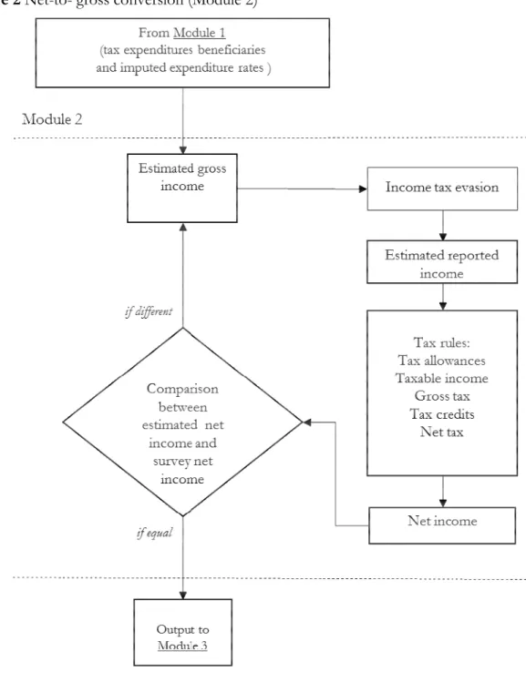
Table 7 considers tax credits, covering both the model-simulated and the imputed ones. In general, BETAMOD estimates provide a good approximation of the tax returns figures.
Table 7 Aggregate validation: tax credits
Number of beneficiares1 Value2
Tax credit BMETAOD- Official tax
returns Diff % BETA -MOD Official tax returns Diff %
Income source tax credit 37,852 36,426 3.9 44,475 41,887 6.2 Dependent family members tax
credit 12,624 12,624 0.0 10,914 11,375 -4.0
19% tax credits
Healthcare expenses 14,855 15,002 -1.0 2,588 2,585 0.1
Mortgage interest payments on
main residence 3,817 3,841 -0.6 1,146 1,147 0.0
Life insurance premium 6,437 6,520 -1.3 750 751 -0.1
Secondary and tertiary education 2,102 2,095 0.3 318 318 0.0
Funeral expenses 413 428 -3.6 119 119 -0.4
Mortgage interest payments on
other properties 281 296 -5.1 80 77 3.2
Annual enrollment to sports
facilities 1,506 1,522 -1.1 60 60 0.1
Rent for resident students 159 169 -6.2 51 50 1.0
Social/community/home care
expenses 113 108 4.0 38 38 0.6
Charitable donations 899 915 -1.8 36 36 0.3
Real estate brokerage expenses 95 100 -4.1 16 15 1.5
Others 1,080 1,101 -1.9 83 83 -0.1
55% tax credits
For energy conservation's
interventions 1,038 1,052 -1.4 1,351 1,349 0.1
41%-36% tax credits
House refurbishments 5,175 5,267 -1.8 2,242 2,243 0.0
20% tax credit 539 540 -0.1 65 65 -0.1
Others tax credits
For tenants subject to controlled rent and for employees relocating
closer to work 708 713 -0.7 138 136 1.5
Security sector tax credit 375 349 7.5 50 50 0.0
Others 158 137 15.3 84 83 1.6
The number of beneficiaries and the amount of the income-source tax credit are overestimated of about 3.9% and 6.2% respectively. This is mainly due to the fact that estimated reported incomes are more dense in the bottom of the distribution in BETAMOD than in tax data. Since the
tax credit is decreasing in income, the BETAMOD tax credit results greater than in tax returns data.
As to the dependent family members tax credit, the striking similarity in the number of beneficiaries is motivated by this variable having been taken into account in the weighting design, while the simulated amount of tax credit is -4.0% lower than the official figure, presumably reflecting the sample distribution of household composition, relevant for identification of dependants. The other most sizeable tax credits, namely healthcare expenditures23, house
refurbishment, energy interventions and mortgage interest tax credits are remarkably close to the administrative figures. As expected, the main discrepancies arise in the numbers of beneficiaries of the less sizeable tax credits24.
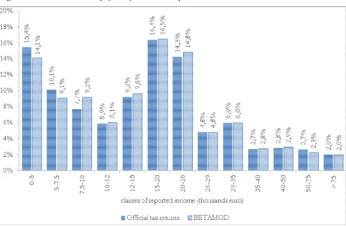
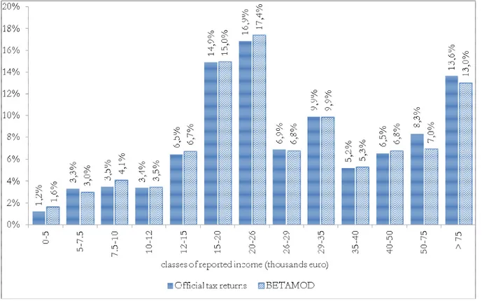
Besides assessing the model validity at the aggregate level, no less attention should be devoted to the validation of the distributional patterns of different components of the model output, as it mainly represents a tool for carrying out distributional analyses. First, we compare the distribution of taxpayers (Figure 3) and of simulated reported income (Figure 4) with official statistics. Overall, the BETAMOD distributions are strikingly similar to the fiscal data ones,
especially in the classes of reported income where most of taxpayers fall (12-26 thousands of euros). Such pattern of similarity is confirmed when considering the distribution of average gross and net tax liabilities across income classes (Table 8).
The following Figures 5 and 6 represent the progressive design of the income source and the family dependents tax credits, as arising from BETAMOD and from tax returns data. Again, the
similarity between the two is striking, and is also confirmed for other tax allowances (the related figures are reported in Appendix C). Interestingly, both tax credits are partly lost by taxpayers in the bottom income class, due to their low level of taxable income/gross tax liability, and to the non-refundable nature of these tax credits.
As evidenced in previous Tables 6 and 7, tax deductions and tax credits subsidize personal spending on a wide range of goods and services, including housing, healthcare and education. Some preliminary information on the model assessment of the redistributive impact of those tax reliefs that substitute direct expenditures25 is provided in Table 9. Were tax expenditures
abolished, state and local tax revenue would be raised by 15,100 millions of euros (+10% with
23 Among tax credits granted for specific expenditures, healthcare expenditures represents about the 49%.
24 Simulating the correct number of beneficiaries in the quantitatively less important tax credits is, in fact, one of the
most common challenges in microsimulation modelling due to the lack of information relevant for identification of potential claimants in the survey data, as well as to the small number of individuals involved.
respect to the baseline simulation) and inequality indexes reduced of about 0.35%. Although the “revenue method” does not account for taxpayers’ behavior (see, Burman et al., 2008), deductions and tax credits appear to generate a more unequal distribution of households’ equivalent disposable income26.
Figure 3 Distribution of taxpayers by classes of reported income
26 We compute household’s disposable income by adding all true gross income earned by the family members ad
subtracting the personal tax liabilities. The household equivalent income is obtained by applying the OECD-modified
Figure 4 Distribution of reported income by classes of reported income
Table 8 Gross and net tax distribution by income classes (mean values in euros)
Classes of reported income (euros)
Gross tax Net tax
BETAMOD Official tax returns BETAMOD Official tax returns
0 – 5,000 442 453 281 229 5,000 - 7,500 1,317 1,394 613 460 7,500 - 10,000 1,851 1,938 415 492 10,000 - 12,000 2,437 2,417 826 867 12,000 - 15,000 2,998 2,993 1,384 1,426 15,000 - 20,000 4,005 3,988 2,373 2,336 20,000 - 26,000 5,363 5,359 3,745 3,673 26,000 - 29,000 6,612 6,584 5,026 4,952 29,000 - 35,000 7,979 7,966 6,403 6,401 35,000 - 40,000 10,077 9,962 8,763 8,513 40,000 - 50,000 12,634 12,439 11,452 11,169 50,000 - 75,000 18,111 18,244 17,134 17,228 above 75,000 45,707 46,799 44,166 45,551 Average 4,993 5,262 4,744 4,837
Figure 5 Income source tax credit as a proportion of reported income (%)
Table 9 Effect on inequality of tax expenditures
Tax law 2010
Gini index 32.55%
Atkinson index 18.35%
Removal of deductions Variation
Gini index 32.32% -0.23%
Atkinson index 18.14% -0.20%
Removal of tax credits Variation
Gini index 32.40% -0.15%
Atkinson index 18.20% -0.14%
Removal of both deductions and tax credits Variation
Gini index 32.17% -0.38%
Atkinson index 17.99% -0.35%
5. Tax evasion and its distributional profile
To showcase BETAMOD potential for analysis, in this section we provide some distributional
evidence on tax evasion. According to our estimates, on aggregate €61 billions of gross income escape tax authorities, corresponding to a tax revenue loss amounting to about €16 billions27.
Unsurprisingly, tax evasion arises mostly from self-employed income and, to a lesser extent, rental income from property: overall, 85% of evaded income is attributable to these two sources (65% and 20% respectively). The remaining 15% of evaded income is attributable to employment income, as pension income, representing a public transfer, can hardly be hidden from tax authorities.
Average tax evasion rates, by income source and geographical area, are reported in Table 10. The figures reveal that tax evasion on employment income, while not negligible, is low (2.9%), and that the largest tax evasion rates are registered on rental income from immovable property (33.6%) and self-employment income (24%). Relevant differences arise also between geographical areas: in particular, our results identify individuals living in the South of Italy as those displaying systematically higher tax evasion rate, followed by those in the North East. The BETAMOD estimated average values are slightly lower, yet not inconsistent, with estimates derived
by above mentioned studies on tax evasion in Italy.
27 The tax revenue loss refers to the personal income tax (15 billions), regional and municipal additional income taxes
Table 10 Average tax evasion rates by income source and geographical area (%)
Average tax evasion rate NW NE C S Italy
Employment income 2.7 3.1 2.8 3.3 2.9
Pensions 0.0 0.0 0.0 0.0 0.0
Self-employment income 22.2 25.1 22.3 27.2 24.0
Rental income from immovable property 30.6 35.5 31.3 38.2 33.6
Total income 6.9 7.5 6.8 7.7 7.2
As arises from Figure 7 (a,b,c), the distribution of tax evasion rates varies across different income sources. Among individuals who hide employment income from tax authorities, low tax evasion rates are most often estimated. On the contrary, more than half of self-employed income tax evaders display a tax evasion rate that is higher than 60%. A similar distribution arises for rental income evasion; about 50% of rental income tax evaders display tax evasion rates between 60 and 80%. Figure 7d plots the full distribution of estimated individual tax evasion rates, by true gross income, i.e. the ‘true’ amount individuals would report to tax authorities under full compliance. The Figure reveals that individuals’ tax evasion rates cluster around an upper and a lower level, reflecting the underlying individual income sources composition, i.e. the prevalence of employment (relatively low level of tax evasion) versus self-employed and rental incomes (high level of tax evasion). The evidently negative gross income gradient of tax evasion rates clearly reflects the tax evasion estimation procedure, which accounts for evasion-by-income profiles28.
The following Figure 8, where tax evasion rates by income class are shown, provides further evidence on the negative gross income gradient of tax evasion rates, and allows to better gauge the income profile of tax evasion behaviour by income source as well. In relative terms, both for each income source, and for their aggregate, consistently with previous studies, BETAMOD
reflects tax evasion rates generally decreasing in income29 (although to a much lesser extent in the
lowest income classes, with respect to other classes).
28 As previously explained in section 3.4, the decreasing aggregate profile results by the comparison
between BETAMOD simulated gross income and reported income to tax authorities.
29 Results must be considered taking into account that they are based on the income distribution which directly
emerges from IT-SILC survey. However, the survey doesn’t guarantee representation of true income distribution. Previous studies, although based on Bank of Italy’s survey (e.g. Cannari and D’Alessio, 1992) have in particular identified two major biases, which are indeed common to surveys conducted in other countries. The first is the selectivity bias due to the fact that not all families are equally available to participate to the survey; the second is known as under-reporting, and arises when the respondent reports a disposable income below the true income. Both selectivity bias and under-reporting can explained with the fear that some people have that their files could be accessed by the tax authorities. Evidence indicates that the fear is more pronounced in individuals belonging to the upper tail of the distribution. A third, though less relevant, bias is originated by some over-reporting of people belonging in the lower tail. Clearly all three biases contribute to making the sample distribution less unequal than the real distribution.
Figure 7 Distribution of tax evasion rates by type of income (tax evaders only, in percentage)
tax evasion rate 30.8 21.6 19.1 13.9 9.2 4.5 0.9 0.0 0.2 0.4 0.6 0.8 1.0
tax evasion rate 0.3 0.8 1.6 5.6 14 24.1 31.9 21.1 0.5 0.0 0.2 0.4 0.6 0.8 1.0
a) employment income b) self-employment income
tax evasion rate
2 1.5 1.7 4.4 9.2 19.6 27.5 28.2 5.8 0.0 0.2 0.4 0.6 0.8 1.0 0 20 40 60 80 100 0. 0 0. 2 0. 4 0. 6 0. 8 1. 0
true gross income (x 1000)
ta x e va si o n r a te
Figure 8 Average tax evasion rates by type of income and by true gross income classes
Figure 9 shows the total amount of unreported income. It can be noticed that, despite the decreasing profile of tax evasion rates, most of evaded income is due to taxpayers with gross income in the range 12,000-50,000 euro, and mainly to self-employed income.
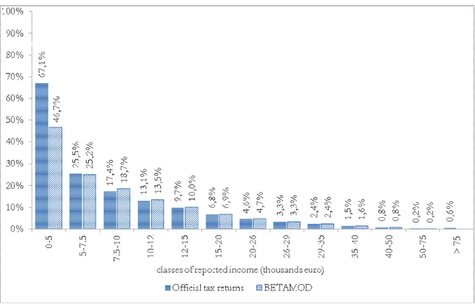
Tax evasion, by reducing reported income, causes a relevant downward shift in the distribution of taxpayers by reported income, with respect to that by (true) gross income. To begin with, tax evasion may modify the relative position (in terms of reported income) between fully-compliant taxpayers and same-true-gross-income evaders, generating an horizontal inequity effect in income taxation. Indeed, while horizontal inequity is one of the major consequence of tax evasion, very little studies measuring it exist.
BETAMOD evidence is provided in Figure 10, where the two cumulative distributions of
taxpayers, by (true) gross and reported income respectively, are shown. The distribution of individuals by reported income is thicker in the left tail, when compared with the distribution of gross income, suggesting a downward movement, along the income distribution, of taxpayers who “benefit” from tax evasion.
Figure 9 Unreported income by classes of true gross income (millions of euros)
Figure 10 Cumulative distributions of taxpayers by (true) gross and reported income classes
BETAMOD transition matrix, reporting the share of true gross income taxpayers falling in each
income class, found in different reported income classes as a result of tax evasion, is reported in Table 11. As a result of non-compliance, the taxpayers in the bottom income class, for instance, moves from about 10% when considering true gross income to about 14% when considering reported income relevant for taxation. Evaders who enter the bottom income class come from the 2nd to the 8th income class (up to 29 thousands of euros), rather than from higher income
classes, reflecting the decreasing income profile of tax evasion rates. Moving to the upper classes, we observe a similar pattern of shifts across income classes, although the number of shifts is progressively reduced, again because of the negative income gradient in tax evasion. While Table 10 only reports between class shifts, building on the availability of individual tax evasion rates, BETAMOD allows to detect further shifts happening within each income class.
Once taxation applies to reported income, shifts along the income distribution, give rise not only to horizontal inequities, but also to a re-ranking effect, with a reversal of taxpayers’ relative positions before (i.e. reflecting the true gross income position) and after personal income taxation ( i.e. based on the reported income position ), which the model also allows studying. Although preliminary, the novel empirical evidence showcased here bears major implications for the accurate measurement of the actual redistributive effect of personal income taxation and its decomposition in the horizontal, vertical and re-ranking effect, each of which is possibly altered by tax evasion.
Table 11 Transition matrix of taxpayers from (true) gross income to reported income (%) Classes of true gross income
0-5 5-7.5 7.5-10 10-12 12-15 15-20 20-26 26-29 29-35 35-40 45-50 50-75 > 75 Total Cl as se s of r ee po rt ed in co m e 0-5 10.47 1.51 0.79 0.33 0.57 0.33 0.11 0.01 14.11 5-7.5 6.37 0.91 0.43 0.42 0.52 0.32 0.07 0.04 9.08 7.5-10 7.13 0.60 0.49 0.34 0.39 0.11 0.08 0.02 9.15 10-12 4.38 0.71 0.50 0.25 0.06 0.11 0.04 0.01 6.06 12-15 7.66 1.25 0.31 0.08 0.17 0.09 0.04 9.61 15-20 14.26 1.64 0.24 0.19 0.09 0.05 16.5 20-26 13.43 0.72 0.43 0.12 0.11 0.01 14.82 26-29 4.06 0.51 0.12 0.08 0.01 4.78 29-35 5.34 0.37 0.23 0.06 6.01 35-40 2.38 0.31 0.05 2.75 40-50 2.64 0.30 2.94 50-75 2.25 0.02 2.26 > 75 1.95 1.95 Total 10.47 7.88 8.83 5.74 9.85 17.21 16.45 5.36 6.86 3.23 3.48 2.67 1.96 100
References
Aronson J.R. and Lambert P.J. (1994), Decomposing the Gini coefficient to reveal vertical, horizontal and reranking effects of income taxation, National Tax Journal, vol. 47, pp. 273-294.
Atkinson A. B., Gomulka J. and Sutherland H. (1988), Grossing-up FES data for Tax-Benefit Models, in Atkinson A.B. and Sutherland H. (1988), Tax-Benefit Models, STICERD Occasional Paper,No. 10, London. London School of Economics, STICERD.
Avram S. (2014), The distributional effects of personal income tax expenditure, EUROMOD Working Paper Series, EM14/14.
Bacharach M. (1965), Estimating Nonnegative Matrices from Marginal Data, International Economic
Review, 6 (3), pp. 294–310.
Baldini M., Ciani E. and Pacifico D. (2011), MAPP, a tax benefit microsimulation Model for the Analysis
of Public Policies in Italy, University of Modena and Reggio Emilia, Department of
Economics.
Bank of Italy (2012), Household Income and Wealth in 2010, Supplements to the Statistical Bulletin, n. 6.
Bernasconi M. and Marenzi A. (1997). Gli effetti redistributivi dell'evasione fiscale in Italia.
Ricerche quantitative per la politica economica, Bank of Italy, Rome, pp. 1-38.
Betti G., Donatiello G. and Verma, V. (2011), The Siena microsimulation model (SM2) for net-gross conversion of EU-SILC income variables, International Journal of Microsimulation, 4 (1),
pp. 35-53.
Bourguignon F. and Spadaro A. (2006), Microsimulation as a tool for evaluating redistribution policies, Journal of Economic Inequality, 4, pp. 77-106.
Burman L. (2003 ), Is the Tax Expenditures Concept Still Relevant?, National Tax Journal, LVI (3), pp. 613-627.
Burman L., Geissler C. and Toder E. (2008), How Big Are Total Individual Income Tax Expenditures, and Who Benefits from Them?, American Economic Review: Papers &
Proceeding, 98 (82), pp.79-83.
Ceriani L., Fiorio C.V. and Gigliarano C. (2013), The Importance of Choosing the Data Set for
TaxBenefit Analysis, EUROMOD Working Paper No. EM 5/13.
D’Amuri F. and Fiorio C. (2006), Grossing-up and validation issues in an Italian tax-benefit
microsimulation model, Econpubblica WP, No. 117, Bocconi University, Milan, December.
Fiorio C. and D'Amuri F. (2006), Tax Evasion in Italy: An Analysis Using a Tax-benefit Microsimulation Model, The ICFAI Journal of Public Finance, May, pp. 19-37.
Getzen T. (2000), Health care is an individual necessity and a national luxury: applying multilevel decision models to the analysis of health care expenditures, Journal of Health Economics, 19(2), pp. 259-270.
Immervoll, H. and O'Donoghue C. (2001), Imputation of gross amounts from net incomes in household
surveys: An application using EUROMOD, EUROMOD Working Paper Series, No.
EM1/01.
ISTAT (2014), Multiscopo Survey on Health Conditions and the Use of Health Services 2012/2013, http://www.istat.it/it/archivio/7740.
Keen M., de Mooij R., Eyraud L., Tyson J., Bond S. and Walters L. (2012), Italy: the Delega Fiscale
Marino M.R. and Zizza R. (2012), Personal Income Tax Evasion in Italy: An Estimate by Taxpayer Type, in Pickhardt M. and A. Prinz (eds.) Tax Evasion and the Shadow Economy, Cheltenham, UK: Edward Elgar Publishing.
Mazzaferrro C. and Morciano M. (2008), CAPP_DYN: A Dynamic Microsimulation Model for the
Italian Social Security System, CAPPaper n. 48.
Ministry of Economy and Finance (MEF) (2011), Gruppo di lavoro sull’erosione fiscale: Relazione Finale,
Roma, November 2011.
Mitton L., Sutherland H. and Weeks M. (2000), Microsimulation Modelling for Policy Analysis. Challenges
and Innovations, Cambridge University Press, Cambridge.
Murphy K. (2012), Closing the European Tax Gap, Tax Research LLP.
Newhouse J. P. (1977), Medical care expenditure: A cross-national survey, Journal of Human
Resources, 12, pp. 115–125.
Pellegrino S., Piacenza M. and Turati G. (2011), Developing a static microsimulation model for the analysis of housing taxation in Italy, International Journal of Microsimulation, 4(2), pp. 73-85.
Poterba J. M. (2011), Economic Analysis of Tax Expenditures, National Tax Journal, 64 (2), pp. 451-458.
Rubin D. (1980), ‘Bias reduction using Mahalanobis-metric matching’, Biometrics, 36, pp. 293–298. Sutherland H. and Figari F. (2013), EUROMOD: the European Union tax-benefit
microsimulation model, International Journal of Microsimulation, 6 (1), pp. 4-26.
Tyson J. (2014), Reforming Tax Expenditures in Italy: What, Why, and How?, IMF Working paper, WP/14/7.