Generalize policy on supporting user scenario

Alma Mater Studiorum

_{· Universit`a di}

Bologna

SCUOLA DI SCIENZE

Corso di Laurea Magistrale in Informatica

Generalize Policy

on

Supporting User Scenario

Relatore:

Chiar.mo Prof.

Mauro Gaspari

Presentata da:

Lorenzo Cazzoli

Sessione II

Anno Accademico 2016/2017

a ... Cazzoli

mio nipote,

che nascer´a in questi giorni

Abstract

In this thesis we present a way of combining previously learned robot be-havior policies of di↵erent users. The main idea is to combine a set of policies, in tabular representation, into a final sub-optimal solution for the problem all users have contributed to. We assume that the features/di↵erences of users are unknown and need to be extracted from the di↵erent policies generated from same user. This information is used to weight the importance of a set of actions to sum up two policies.

The proposed approach has been tested on a virtual environment finding out that the combined policy works as a general policy suitable for all users, as it always selects actions that are satisfying the users at the border of the defined sensorial possibilities.

All the assumptions has been finally verified on a real environment finding out all the limitations of the proposed model.

Sommario

La Human-Robot-Interaction ´e un area di studio che coinvolge diverse discipline. Le di↵erenti categorie di possibili target condizionano il tipo di sfida a cui si ´e posti di fronte. Per esempio, piattaforme robot pensate per i bambini devono adattarsi alle loro capacit´a comunicative e al loro comporta-mento in continua evoluzione. Al contrario piattaforme per persone anziane devono adeguarsi ad eventali deficit delle capacit´a visive ed uditive. I robot hanno bisogno di potersi adattare alle capacit´a e deficit delle persone con cui stanno interagendo. Ci si aspetta che nel caso di utenti con problemi alla vista, il robot usi pi´u suggerimenti vocali, mentre per utenti con problemi uditivi siano usate le mimiche facciali e altri movimenti.

Attraverso l’uso del Reinforcement Learning [Sutton and Barto(2011)] i robot possono facilmente imparare il comportamento corretto per ogni gruppo di utenti indipendentemente dalle loro di↵erenze sensoriali. Il pro-blema ´e che le informazioni imparate dall’interazione con uno di questi non possono essere usate nel processo di apprendimento di un altro, poich´e il secondo utente potrebbe avere diverse capacit´a e quindi non garantire che le azioni siano percepite nello stesso modo causando gli stessi risultati. Le policy imparate permettono al robot di comportarsi correttamente solo con l’utente corrente, ma quando il robot ´e di fronte a un nuovo utente, deve aggiornare la sua policy per adattarsi alla nuova situazione. Se i due utenti non sono troppo diversi, il robot ´e in grado di generare una nuova policy affidabile, mentre, nel caso contrario, il comportamento generato potrebbe

iv

essere fuorviante a causa dell’imprecisione della policy.

Combinando le policy vogliamo superare questo problema garantendo che il robot si comporti correttamente, con un comportamento sub-ottimale, con tutti gli utenti incontrati e senza il bisogno di imparare una policy da zero per i nuovi. Questo fatto ´e ancora pi´u importante quando si impara online interagendo con persone che sono sensibili agli errori e al passare del tempo. In questo caso la policy combinata ´e usata per inizializzare il processo di apprendimento, accelerandolo e limitando gli errori dovuti all’esplorazione iniziale.

In questa ricerca presentiamo un modo per combinare policy di utenti diversi precedentemente apprese. L’idea ´e di combinare un insieme di policy, rappresentate in forma tabulare, in una soluzione sub-ottimale al problema a cui tutti gli utenti hanno contribuito. Nel fare ci´o assumiamo che le carat-teristiche degli utenti siano sconosciute e quindi necessitino di essere estratte dalle di↵erenze evidenziate dal comfronto di policy generate interagendo con lo stesso utente. Le informazioni estratte in questo modo sono usate per pesare l’importanza delle azioni scelte per l’utente nel processo di policy combination.

Per iniziare sono state raccolte le policy da utenti simulati che dove-vano completare il gioco del memory, assistiti da un agente virtuale. Ogni volta che l’utente cercava una coppia sull’area di gioco, l’agente, che era a conoscenza della posizione della carta da trovare, lo aiutava suggerendo la direzione o l’area del tabellone in cui tentare. Per permettere l’adattamento del comportamento dell’agente, si ´e utilizzato un algoritmo di apprendimento chiamato Q-learning insieme alla tecnica ✏-greedy per bilanciare exploration ed exploitation [Watkins and Dayan(1992)]. La comunicazione ´e stata imple-mentata tramine la simulazione di azioni multimodali composte da sguardo, voce, movimenti della testa ed espressioni facciali.

SOMMARIO v Un insieme di personas [Schulz and Fuglerud(2012)] ´e stato generato per coprire i diversi tipi di utenti e capire i loro bisogni. Tramite le storie di ogni personas ´e stato estratto un set di caratteristiche usato per definire il comportamento degli utenti virtuali. Per esempio un utente sordo ignorer´a tutti i suggerimenti vocali e seguir´a solo le altre parti delle azioni multimodali. La bont´a dei risultati ottenuti nelle simulazione dello scenario, ci ha mo-tivato ad estendere la ricerca con test sullo scenario reale. Questo ´e stato realizzato utilizzando una piattaforma touch, su cui sono state disposte le carte del memory, posizionata di fronte a FurHat, il robot usato per intera-gire con l’utente. Un gruppo di volontari ´e stato usato per la raccolta dei dati, da cui ´e stata generata la combined policy utilizzata su un gruppo al-largato di volontari al fine di validare i risultati ottenuti dalle simulazioni con le personas e quindi l’algoritmo proposto.

La tesi ´e divisa nei seguenti capitoli: nel capitolo 2 viene fornita una panoramica delle ricerche correlate; il capitolo 3 introduce le basi teoriche richieste per lo studio in questione; il capitolo 4 presenta lo scenario utiliz-zato nei test, la cui implementazione ´e trattata nel capitolo 5; nel capitolo 6 e 7 sono riportate le scelte e risultati relativi alle simulazioni e↵ettuate rispettivamente nello scenario virtuale e reale; il capitolo 8 riporta una breve riflessione conclusiva e le possibili direzioni future della ricerca.

Contents

3 Background & Concept 9 3.1 Policy Generation . . . 10

3.1.1 Q-learning . . . 10

3.1.2 SARSA . . . 11

3.1.3 LSPI . . . 11

3.2 Policies Combination . . . 14

3.2.1 User Informations Extraction . . . 14

3.3 Speed Up the Learning . . . 15

4 Scenario 17 4.1 State Representation . . . 19

4.2 Action Space . . . 22 vii

viii CONTENTS

4.3 Reward Function . . . 25

5 Implementation 27 5.1 Online RL algorithms . . . 27

5.1.1 Q-learning same as SARSA . . . 27

5.1.2 Online LSPI . . . 29

5.2 Policy Combination . . . 31

5.2.1 User Informations Extraction . . . 31

5.2.2 Combination Algorithm . . . 34

5.3 Policy Reuse Adaptation . . . 36

6 Virtual Simulation 39 6.1 Adaptation of Implementation . . . 39 6.1.1 Virtual Environment . . . 40 6.1.2 Virtual Agent . . . 40 6.1.3 Fictional User . . . 41 6.2 Procedure . . . 44 6.3 Results . . . 45 6.4 Discussion . . . 50 7 Human World 55 7.1 Adaptation of implementation . . . 55 7.1.1 User . . . 56 7.1.2 Central Logic . . . 56 7.1.3 Touch Screen . . . 57 7.1.4 Furhat . . . 58 7.2 Procedure . . . 58 7.3 Results . . . 60 7.4 Discussion . . . 64 8 Conclusion 71 List of Figures 75

CONTENTS ix List of Algorithms 77 List of Tables 79 A Personas 81 B Suggestion Interpretation 91 C Furhat 93

Summary of Notation

Capital letters are used for random variables and major algorithm vari-ables. Lower case letters are used for the values of random variables and for scalar functions. Quantities that are required to be real-valued vectors are written in bold and in lower case (even if random variables).

s state a action

S set of nonterminal states

S+ _{set of all states, including the terminal state}

A(s) set of action possible in state s t discrete time step

St state at t

At action at t

Rt reward at t

⇡ policy, decision making rule

⇡(s) action taken in state s under deterministic policy ⇡ w set of parameters

basis functions

w⇡ parameters for the approximated function of ⇡

v⇡ expected return under policy ⇡

xii CONTENTS v⇡(s) value of state s under policy ⇡

ˆ

Q(s, a, w) approximate value of state-action pair s, a given weight w ↵ learning rate parameter

discount rate parameter

✏ probability of random action in ✏-greedy policy

Chapter 1

Introduction

Human-Robot-Interaction is an increasingly studied field with many dis-ciplines involved. The di↵erent categories of targets influence the type of challenges that need to be accomplished. For instance, robot platforms de-signed for children have to adapt to their maturing behavior and commu-nication abilities. On the other hand, platforms for elderly people have to accommodate to the digressive visual and hearing capacities. The robots need to adapt their behavior to the capabilities and deficits of their interac-tion partners. It is expected that if the user has some visual lack the robot will use more voice suggestion and in the opposite case, with lacking hearing abilities, more facials expressions or gestures are required.

Using Reinforcement Learning [Sutton and Barto(2011)] robots can easily learn the correct behavior for each group of users independently from their sensorial di↵erences. The problem is that information learned interacting with one user can’t be used in a learning process of another user because they presumably have di↵erent capabilities, thus it is not guaranteed that two actions are perceived in the same way and cause the same results. The learned policy allows the robot to infer a correct behavior only for the current user. The way in which the user is interacting and interpreting the agent’s ac-tions define the problem and the learned behavior. When the robot interacts

2 1. Introduction with a new user it has to update its policy to adapt to the new situation. If the two users are not too di↵erent, the robot is able to generate a new reliable behavior policy. Otherwise the generated behavior could be mislead-ing or frightenmislead-ing due to an inaccurate policy. An agent that has to assist multiple and di↵erent users has to learn di↵erent behavior for each user. In addition is required a method to recover already learned behavior for users whose presence recurs more than one time. This is not immediate because it need memory to store the learned policies and an identification system to recognize each user.

Combining policies we can overcome this problem guaranteeing that the robot behaves properly, with a sub-optimal solution, with all encountered users and without the need to learn again a policy from scratch for the cur-rent user. This fact is even more important when the system has to interact with humans. In this case the combined policy is used to initialize the learn-ing process, with the target of speed up the learnlearn-ing and limit the initial wrong suggestions due to exploration.

In the past di↵erent solutions have been tested to speed up the learning on di↵erent tasks performed by the same user. Examples of there are [Taylor and Stone(2009), Sherstov and Stone(2005), Fern´andez and Veloso(2006), Konidaris and Barto(2006)] where the information learned about a task are used in the resolution of a similar one. They are all interesting approaches, but they are not suitable for the problem that we have in question, since we are working with di↵erent users and they are thought to work in di↵erent task of the same user.

The policies combination is similar to the combination of the policies per-formed by an arbitrator on the information learned by the di↵erent subagents. This combination techniques are used by [Russell and Zimdars(2003), Rosen-blatt(2000)] in order to find new way to select the optimal action in dis-tributed scenarios.

3 For a successful combination of the policy is important to understand the deficits of the user situated in front of the agent. this is important to make the correct use of policy learned on him. No one would take in considera-tion the visual suggesconsidera-tions learned during the interacconsidera-tion with a blind user. Understand the users is vital to understand the di↵erent way on which the users tackle the problem and this knowledge is used to find a common inter-pretation that defines the base of a general behavior. In all the situations where di↵erent users react to di↵erent actions the optimal action need to be selected between the performed actions. If the scenario include multimodal actions every user can influence the final action with parts of his behavior, the parts on which his senses are not lacking in perception.

As in [Griffith et al.(2013)Griffith, Subramanian, Scholz, Isbell, and Thomaz, Thomaz and Breazeal(2008)] human feedback can be used, in the online learning, to improve the quality of the reward and to drive the training of the agent. Used in the correct ways they can also accelerate the learning obtaining good policies even after few rounds.

The goals of this thesis can be summarized in find an implementation of the policy combination algorithm in order to:

1. Use the same policy for multiple users

2. Decrease the time required for online training.

The rest of the thesis is structured as follow: in chapter 2 an overview of recent research organized in three categories is given. They are divided on groups that are concerning the di↵erent phases of our research. In the chapter 3 are introduced the concepts and the theoretical background required for the studies. The scenario used for the simulation is presented in the chapter 4, while all the implementations are illustrated in the chapter 5. Chapters 6 and 7 are reporting the choices and results of the simulations performed

4 1. Introduction on the virtual and real world scenarios. The last chapter, the number 8, presents the conclusion and future works.

Chapter 2

Related Work

In the recent past there aren’t similar works done in the research com-munities, that is instead focused on di↵erent forms of knowledge transfer.

In this chapter we will first cite some of these and after we will see some approaches used to solve di↵erent research questions, from which we have taken inspiration. The last section are works that explain how human feed-back can be used to improve online training.

2.1

Transfer of Knowledge

The reinforcement learning paradigm is a popular way to address prob-lems that have only limited environmental feedback, rather than correctly labeled examples, as is common in other machine learning contexts. While significant progress has been made to improve learning in a single task, the idea of transfer learning has only recently been applied to reinforcement learning tasks. The core idea of transfer is that experience gained in learning to perform one task can help improve learning performance in a related, but di↵erent, task. [Taylor and Stone(2009)] present a framework that classifies transfer learning methods in terms of their capabilities and goals, and then use it to survey the existing literature, as well as to suggest future directions for transfer learning work.

6 2. Related Work In the paper of [Sherstov and Stone(2005)] is presented action transfer, a novel approach to knowledge transfer across tasks in domains with large action sets. They demonstrate the use of knowledge transfer between related tasks to accelerate learning with large action sets. The algorithm rests on the idea that actions relevant to an optimal policy in one task are likely to be relevant in other tasks. Their technique extracts the actions from the optimal solution to the first task and uses them in place of the full action set when learning any subsequent tasks. When optimal actions make up a small fraction of the domain’s action set, action transfer can substantially reduce the number of actions and thus the complexity of the problem. However, action transfer between dissimilar tasks can be detrimental.

[Fern´andez and Veloso(2006)] contribute Policy Reuse as a technique to improve a reinforcement learning agent with guidance from past learned sim-ilar policies. Their method relies on using the past policies as a probabilistic bias where the learning agent faces three choices: the exploitation of the on-going learned policy, the exploration of random unexplored actions, and the exploitation of past policies. Policy Reuse also identifies classes of similar policies revealing a basis of core policies of the domain. They demonstrate that such a basis can be built incrementally, contributing the learning of the structure of a domain.

[Konidaris and Barto(2006)] introduce the use of learned shaping rewards in reinforcement learning tasks, where an agent uses prior experience on a sequence of tasks to learn a portable predictor that estimates intermediate rewards, resulting in accelerated learning in later tasks that are related but distinct. Such agents can be trained on a sequence of relatively easy tasks in order to develop a more informative measure of reward that can be trans-ferred to improve performance on more difficult tasks without requiring a hand coded shaping function.

2.2 Composite Agent 7

2.2

Composite Agent

[Russell and Zimdars(2003)] explores a very simple agent design method called Q-decomposition, wherein a complex agent is built from simpler sub-agents. Each subagent has its own reward function and runs its own rein-forcement learning process. It supplies to a central arbitrator the Q-values for each possible action. The arbitrator selects an action maximizing the sum of Q-values from all the subagents. This approach has advantages over designs in which subagents recommend actions. It also has the property that if each subagent runs the Sarsa reinforcement learning algorithm to learn its local Q-function, then a globally optimal policy is achieved.

[Rosenblatt(2000)] introduces a new means of action selection via utility fusion. Distributed asynchronous behaviors indicate the utility of various possible states and their associated uncertainty. A centralized arbiter then combines these utilities and probabilities to determine the optimal action based on the maximization of expected utility. The construction of a utility map allows the system being controlled to be modeled and compensated for.

2.3

Human Feedback

While Reinforcement Learning (RL) is not traditionally designed for in-teractive supervisory input from a human teacher, several works in both robot and software agents have adapted it for human input by letting a human trainer control the reward signal. [Thomaz and Breazeal(2008)] ex-perimentally examine the assumption underlying these works, namely that the human given reward is compatible with the traditional RL reward sig-nal. This work demonstrates the importance of understanding the human-teacher/robot-learner partnership in order to design algorithms that support

8 2. Related Work how people want to teach and simultaneously improve the robot’s learning behavior.

[Griffith et al.(2013)Griffith, Subramanian, Scholz, Isbell, and Thomaz] argue for an alternate, more e↵ective characterization of human feedback: Policy Shaping. They introduce Advise, a Bayesian approach that attempts to maximize the information gained from human feedback by utilizing it as direct policy labels. With these advancements this paper may help to make learning from human feedback an increasingly viable option for intelligent systems.

Chapter 3

Background & Concept

Reinforcement leaning is learning what to do, how to map situation to action so as to maximize a numerical reward signal. The learner is not told which actions to take but instead must discover which actions yield the most reward by trying them. In the most interesting and challenging cases, actions may a↵ects not only immediate reward but also the next situation and all subsequent rewards. These two characteristics trial and error and delayed reward are the two most important distinguish features of reinforce-ment learning.

Reinforcement learning is di↵erent form supervised learning since it is not learning from examples provided by a knowledgable external supervisor, but it is able to learn from its own experience. The agent is located in an uncharted territory where it must be able to learn independently.

The methods presented in section 3.1.1 and 3.1.2 are today the most widely used reinforcement learning methods. This is probably due to their great simplicity: a) they can be applied on-line, with a minimal amount of computations, to experience generated from interactions with an environ-ment b) they can be expressed nearly completely by single equations that can be implemented with small computer programs.

In the rest of the chapter we will introduce the algorithms selected for the 9

10 3. Background & Concept policy generation (sec 3.1) and the proposed solution for the policy combina-tion (sec 3.2). In seccombina-tion 3.3 we will see how to use the policy generated with the policy combination algorithm to speed up the learning of a new user.

3.1

Policy Generation

3.1.1

Q-learning

Developed by [Watkins and Dayan(1992)] it is an o↵-policy TD-control algorithm. Its simplest form, one-step Q-learning, is defined by

Q(St, At) Q(St, At) + ↵[Rt+1+ maxaQ(St+1, a) Q(St, At)]. (3.1)

The learned action-value function, Q, directly approximates q⇤_{, the}

opti-mal action-value function, independent of the policy being followed.

The goal of the agent is to maximize its total reward. It does this by learning which action is optimal for each state. The action that is optimal for each state is the action that has the highest long-term reward. This re-ward is a weighted sum of the expected values of the rere-wards of all future steps starting from the current state.

The factor is a number between 0 and 1 ( 0 _{  1 ) called discount} factor and trades o↵ the importance of sooner versus later rewards. A factor of 0 will make the agent considering only the current rewards, while factor near to 1 will make it take advantage of long-term high rewards.

The factor ↵ is also included between 0 and 1 ( 0_{ ↵  1 ). It represent} the learning rate and determines to what extent the new acquired information will override the old information. A factor equal to 0 will make the agent not learning anything, while a factor of 1 will make the agent consider only the most recent information. In fully deterministic environment a learning rate of 1 is optimal, while in stochastic problem is required to decrease the learning rate to zero.

3.1 Policy Generation 11

3.1.2

SARSA

It is a on-policy TD control method that learn action-value function rather than state value function. In an on-policy method we must estimate q⇡(s, a)

for the current behavior policy ⇡, for all states s and action a. This can be done using the TD method [Sutton and Barto(2011), chapter 6, p. 219] for learning v⇡.

In Sarsa an episodes consist of alternating sequence of state and state-action pairs:

Sarsa considers transition from state-action pair to state-action pair and learn the value of state-action pairs. The update function:

Q(St, At) Q(St, At) + ↵[Rt+1+ Q(St+1, At+1) Q(St, At)] (3.2)

is performed after every transition from a non terminal state St. If St+1 is

terminal then Q(St+1, At+1) is defined as zero. This rules uses every element

of the quintuple (St, At, Rt+1, St+1, At+1), that make up a transition from a

state-action pair to the next.

3.1.3

LSPI

Introduced by [Lagoudakis and Parr(2003)], LSPI is an approach to re-inforcement learning for control problems which combines value-function ap-proximation with linear architectures and approximate policy iteration. It learns the state-action value function which allows for action selection with-out a model and for incremental policy improvement within a policy-iteration framework.

The state-action value function is approximated using a linear architec-ture: ˆ Q(s, a, w) = k X i=1 i(s, a)wi = (s, a)Tw. (3.3)

12 3. Background & Concept Though maximization of the approximate value over all actions in A(s) the greedy policy ⇡ can be obtained at any given state s using the formula:

⇡(s) = arg max a2A(s) ˆ Q(s, a) = arg max a2A(s) (s, a)Tw. (3.4) For finite action spaces this is straightforward, but for very large or contin-uous action spaces, explicit maximization over all actions in A(s) may be impractical.

Any policy ⇡ (represented by the basis functions and a set of parameters w) is fed to LSTDQ [Lagoudakis and Parr(2003), section 6] along with a set of samples for evaluation. LSTDQ performs the maximization above as needed to determine policy ⇡ for each s0 of each sample (s, a, r, s0) in the sample set. LSTDQ outputs the parameters w⇡ of the approximate value function

of policy ⇡ and the iteration continues in the same manner.

LSPI would be best characterized as an o↵-line, o↵-policy learning algo-rithm since learning is separated from execution and samples can be collected arbitrarily. On-line and on-policy versions of LSPI are also possible with mi-nor modifications.

Online LSPI

The crucial di↵erence from the o✏ine case is that policy improvements must be performed once every few samples, before an accurate evaluation of the current policy can be completed. In the extreme case, the policy is improved after every transition, and then applied to obtain a new transition sample. Then, another policy improvement takes place, and the cycle repeats. Such a variant of PI1 _{is called fully optimistic. In general, online LSPI}

improves the policy once every several transitions taking the name of partially optimistic.

A second major di↵erence between o✏ine and online LSPI is that, while o✏ine LSPI is supplied with a set of transition samples by the experimenter,

3.1 Policy Generation 13 online LSPI is responsible for collecting its own samples, by interacting with the controlled process.

Tile Coding

Tile coding [Sutton and Barto(2011), chapter 9, p. 225] is an approxi-mation method that is particularly well suited for efficient on-line learning. In tile coding the receptive fields of the features are grouped into exhaustive partitions of the input space. Each such partition is called a tiling, and each element of the partition is called a tile. Each tile is the receptive field for one binary feature.

The computation of the indices of the present features is particularly easy if grid like tilings are used. If we address a task with two continuous state variables the simplest way to tile the space is with a uniform two-dimensional grid:

Given the x and y coordinates of a point in the space, it is computationally easy to determine the index of the tile it is in. The width and shape of the tiles should be chosen to match the width of generalization that one expects to be appropriate.

The number of tilings should be chosen to influence the density of tiles. The denser the tiling, the finer and more accurately the desired function can be approximated, but the greater the computational costs.

14 3. Background & Concept

3.2

Policies Combination

In this section we will introduce the idea behind the policies combination algorithm, that is thought to work with multimodal actions and impaired users.

Figure 3.1: Graphical representation of the policies combination schema. The main idea represented in the figure 3.1 consists of creating a black box able to generate a merged policy from the policies of two di↵erent users. To make it possible the system needs the user information, an object that contains information about gaps and keys factor of the relative user.

The process can be applied to more than two users, because a third user can be combined with the policy obtained from the combination of the first two and the process can be iterated again on a new user. The final merged policy is expected to be suboptimal for all the users that has contribute for.

3.2.1

User Informations Extraction

In an environment with impaired users, where not all the parts of the composite actions can be perceived, it is possible that in two policies of the same user, the same state is associated to di↵erent actions and both are correct.

3.3 Speed Up the Learning 15 to play the memory card games, in the state where the matching card is over the card that the user has a propensity for, the agent can perform two di↵erent actions that are proved to be both corrects. In the first case the agent can suggest with an head movement the left direction while the voice is saying “Maybe Up”. In the second case it can point the correct card with the gaze and say again “Maybe Up”.

Since the user can’t percept visual suggestions, the two action, for him, are identical. We can use this defect in our advantage to identify the user’s gap.

Figure 3.2: Graphical view of the user information extraction schema. The user info extraction algorithm (fig 3.2) compares state by state the actions selected in the di↵erent policies and from that comparisons extracts the features of the user.

3.3

Speed Up the Learning

One of the biggest problems of reinforcement learning in online social sce-narios is the time required for the learning. The rewards are received directly from the users and a long training phase with many wrong suggestions could cause frustration and lose of attention. Using Policy Reuse [Fern´andez and

16 3. Background & Concept Veloso(2006)], a technique for reinforcement learning guided by past policies, we can learn the current policies following a past policy and avoid the initial exploration that slow down the learning.

Policy Reuse algorithm balances among exploitation of the ongoing learned policy, exploration of random actions, and exploration of the past policies. The exploration versus exploitation tradeo↵ defines whether to explore un-seen parts of the space or to exploit the knowledge already acquired during the learning process.

The main algorithm of Policy Reuse is the PRQ-Learning algorithm, a method to probabilistically reuse a set of past policies that solve di↵erent tasks within the same domain. This algorithm is composed by two main parts: a) ⇡-reuse exploration strategy b) similarity function.

The ⇡-reuse strategy is an exploration strategy able to bias a new learn-ing process with a past policy. Its goal is to balance random exploration, exploitation of the past policy, and exploitation of the new policy, as repre-sented in Equation 3.5. a = 8 < : ⇧past(s) w.p. ✏ greedy(⇧new(s)) w.p. 1 (3.5) The ⇡-reuse strategy follows the past policy with probability , and it exploits the new policy with probability of 1 . As random exploration is always required, it exploits the new policy with an ✏-greedy strategy.

The similarity function evaluate which are the policies more similar to the current behavior. These policies will be easily preferred in the future knowledge exploration.

Chapter 4

Scenario

The scenario has to be a representation of the environment in which we want to test the efficiency of the policies combination algorithm. For this reason it need to include a user, a social agent, and a simple task on which both user and agent will interact.

Figure 4.1: Picture of the scenario. It is composed by a user a touch screen with the matching memory game and a social robot.

The task selected for the environment is Memory [Wikipedia(2017)], a 17

18 4. Scenario card game in which all the card are laid face down on a surface and two cards are flipped face up over each turn. The object of the game is to turn over pairs of matching cards. Any deck of playing cards may be used, and in our case it is composed of 9 pairs of similar card as is shown in the figure 4.2. The figure of the card are monochromatic image of leaf. For each kind

Figure 4.2: Memory deck.

of leaf there is at least a di↵erent pair with similar shape or number of sub-leaf. This similarity it is thought to reduce their distinctiveness and make the game harder for a human user. In this way the user, that is trying to complete the game, is more inclined to pay attention to the agent suggestions. As physical agent, Furhat (Appendix C) fits perfectly the problem. Furhat is a back projected robot head capable of speech and head gestures. The agent is connected with the game in order to know at priori the position of the matching card. This information allows to Furhat to learn which is the action that suggest better the card position without the need of remember and explore the game board.

The last part of our test scenario is the user. The user interact with the game and agent to complete the task.

4.1 State Representation 19 An import point is the definition of the dynamics of the environment. User and agent interact between each other to complete the task following the routine illustrated in the figure 4.3. The routine starts with the pick, by the user, of the first card. After this action, while the user continue looking for the right card to complete the pair, the game communicates at the agent the position of the matching card. When the user decides which is his second pick the agent detects his gaze and give him a suggestion. The suggestion is based on the position of the observed card and tries to confirm or move the attention of the user on the right card. In the end the user is free to follow or ignore the agent’s suggestion before selecting the second card.

User selects the first card User decides the second card Agent gives a suggestion User selects the second card

Figure 4.3: User agent interactions routine.

4.1

State Representation

The states are the shape in which we want to represent the problem. A first naive representation could be the position of the cards on the board. At first view it seems a good representation, but if we think about its usability this state representation become impossible to use. In a board of 9 pairs of cards the di↵erent disposition of the cards are 18!₂ . With the selected representation the number of states will be so huge that the learning will result impossible.

A new idea is to use a spatial representation that allows to store in a state the information about the spatial relation between two cards. For example a state can store the information about the relative position of the observed card and the matching card. In this way, knowing the current state, the agent has an idea about the position of the second card. For this representation 9 states have been designed.

20 4. Scenario

TOP

LEFT

TOP

TOP

RIGHT

LEFT

MATCH

RIGHT

BOTTOM

LEFT

BOTTOM

BOTTOM

RIGHT

Figure 4.4: Graphical view of the spatial states representation. The possible states are listed in the figure 4.4. Considering the interac-tions routine (fig 4.3) we can note that the user decides the second card after the identification of an observed card. The spatial state is always evaluated moving the “MATCH” cell of grid of the figure 4.4, and all the grid to fol-low, over the observed card. The cells of the grid border are extended in the direction of their label, to cover the entire game board. Checking the position of the matching card the current state can be founded reading the label of the grid’s cell that is covering it. Three examples of possible states are reported in figure 4.5.

Using that representation and adding a state for all the situations where the number of card turned in the round are di↵erent from 1, we can use 10 states to represent every situation of the game.

4.1 State Representation 21

M

1 O

(a) TOP LEFT

M O 1 (b) TOP RIGHT M O 1 (c) LEFT

Figure 4.5: Spatial state examples.

This is an acceptable states space size, but it doesn’t encode any infor-mation about the game progress. Indeed the game is more complicated at the beginning, when all the cards are covered, and becomes more easy in the final phases when the majority of the pairs are already discovered.

Analyzing better the three examples above we can notice that the number of possible cards in the recognized state are di↵erent. In the figure 4.5a there are 10 cards with the same relative position respect to the observed card. This, for the selected state representation, is the maximum number of positions on which the matching card can be associated to the observed card with the same resulting state. The figure 4.5c show the opposite case where the state can be associated to only one card, and so will be obvious, with the correct suggestion, to match the second card.

To store also this information we can add a number, to the name of the state, in order to save the number of possible cards in the state area. At the place of storing this number we have choose to convert the number of cards in a level. The level are the following:

Level 0 1 covered missing card Level 1 2 or 3 covered missing cards Level 2 more than 3 covered missing cards

The use of the level and not the explicit number avoid problems related to rare states, like for examples “TOP LEFT 10” that can happen only when the observed card is in the corner with the matching card top left and no

22 4. Scenario turned cards in that area. It is easy to understand that these states are difficult to train. Another advantage of the level is that the states space is less than 30, while with the explicit number is around 100.

M W 1

(a) TOP Level 0 (b) LEFT Level 1

M

1 W

(c) TOP LEFT Level 2

Figure 4.6: Spatial state with level examples.

For implementation choice of the board there are states where not all the levels are possible. That states are “TOP” and “BOTTOM” where the the ”Level 2” is not possible and “MATCH” where only the “Level 0” is possible. Now that a clear states representation has been defined we can evaluate the real states size.

size = 9_{⇤ 3 + 1} 5 (4.1) (2⇤ 2 + 1)

= 23

4.2

Action Space

The use of Furhat as agent provides us di↵erent type of actions as speak, move the head, change expression and move the eyes.

In our scenario, these actions can be used to suggest the second card at the user. For example a voice suggestion can say a direction or even the right position of the card while with the head gestures the agent can confirm the idea of the user or move his attention to another area of the board.

For each type of actions we have select a subset of possible suggestions that can be useful in the game and fit the state representation. These subsets

4.2 Action Space 23

Figure 4.7: Graphical view of the possible combination between the di↵erent suggestions families.

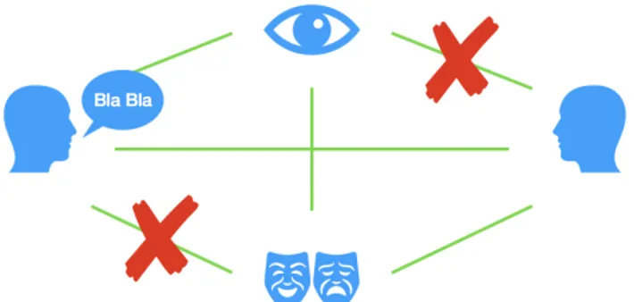
are shown in the tables 4.1 4.2 4.3 4.4. In each of these tables is displayed the code that identifies the suggestion (Code), the action performed by the agent (Suggestion) and the interpretation that we give to that action (Meaning).

Code Suggestion Meaning 0 Say nothing Nothing

1 “It is the right card” The watched card is the matching card 2 “Try at row x and

column y”

The matching card is at the row x and column y

3 “Maybe up” The matching card is up 4 “Maybe down” The matching card is down 5 “Maybe left” The matching card is on the left 6 “Maybe right” The matching card is on the right

Table 4.1: Action: Speech Suggestion

All these suggestions are part of di↵erent subsets that can be combined in composed actions. In figure 4.7 the four blue icons represent the di↵erent suggestion subsets and the green lines the possible combinations. Not all the combinations are significant and so appropriate. For example the connection between the gaze, on the top, and the head movement, on the right, is deleted because while the head is moving is not possible to detect which card the eyes are observing. In the same way, but for a physical reason, also the

24 4. Scenario Code Suggestion Meaning

0 Do nothing Nothing

1 Smile The observed card is the matching card Table 4.2: Action: Face expression

Code Suggestion Meaning 0 Do nothing Nothing

1 Nod The observed card is the matching card 2 Turn to left The matching card is on the left

3 Turn to right The matching card is on the right 4 Turn up The matching card is up

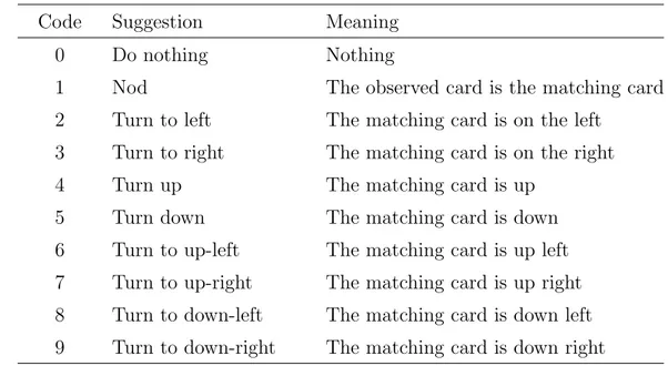
5 Turn down The matching card is down 6 Turn to up-left The matching card is up left 7 Turn to up-right The matching card is up right 8 Turn to down-left The matching card is down left 9 Turn to down-right The matching card is down right

Table 4.3: Action: Head movement

connection between speech suggestion, on the left, and facial expression, on the bottom, is canceled. Indeed during the execution of the selected facial expression (smile) is not possible to speak.

Combining all the size of the suggestion subsets the action space will have size = 7_{⇤ 2 ⇤ 10 ⇤ 2} (4.2)

= 280

but with the use of constrains between the subset family, the final size is equal to 88.

4.3 Reward Function 25 Code Suggestion Meaning

0 Do nothing Nothing 1 Gaze the card at row

x and column y Reveal the position of the matching card Table 4.4: Action: Gaze

4.3

Reward Function

The reward function is one of the essential ingredients for the success of the learning, because from it, depends the fate of each action. As a matter of fact it is thanks to the reward received that the agent understands which actions are good and which are bad for the current state.

Since the goal is to complete the game in less actions possible we want that the user commits no error. To stimulate that behavior we are giving positive reward for each pair found and not a unique big reward for the completion of the game. The reward selected for the agent are the following: +1 Pair match

Chapter 5

Implementation

In the following chapter we will first see the choices and adaptations done during the implementation of the di↵erent RL algorithms. Since in the problem the agent is interacting with a user and the reward and future state are not know at priori, the implemented algorithms are only online. In the second part the code and the concepts behind the policies combination will be largely explained. The last section illustrates the adaptation of the policy reuse algorithm used to speed up the learning.

5.1

Online RL algorithms

The first two algorithms selected are Q-learning and SARSA. Originally they are o✏ine, but thanks to their simplicity they are really easy to adapt in order to work on an online scenario. The third algorithm selected is the online version of LSPI.

5.1.1

Q-learning same as SARSA

During the implementation of the online version of SARSA we have no-ticed that an online version of SARSA was not applicable on the problem. This is due to the fact that, as is possible to see from the figure 4.3, after every action performed by the agent the resulting state is a state where the

28 5. Implementation user has to perform an action. In this state the agent never perform any action so the value of

Q(s, a) = 0 _{8a 2 A(s).} (5.1) If we substitute the hypotheses of the equation 5.1 at Q(St+1, a) in one

step of Q-learning (eq 3.1) and SARSA (eq 3.2) the resulting equations are the following: Q(St, At) = Q(St, At) + ↵[Rt+1+ maxaQ(St+1, a) Q(St, At)] (3.1) Q(St, At) = Q(St, At) + ↵[Rt+1+ 0 Q(St, At)] Q(St, At) = Q(St, At) + ↵[Rt+1 Q(St, At)] (5.2) Q(St, At) = Q(St, At) + ↵[Rt+1+ Q(St+1, At+1) Q(St, At)] (3.2) Q(St, At) = Q(St, At) + ↵[Rt+1+ 0 Q(St, At)] Q(St, At) = Q(St, At) + ↵[Rt+1 Q(St, At)] (5.2)

Both the resulting equations are the same, so has no sense to implement both the algorithms. For this reason, in the test, only Q-learning has been implemented.

Online Q-learning

The Q-learning algorithm is shown in procedural form in algorithm 1. The procedure starts by setting all the values of the Q matrix to 0 and goes trough each step of each episode to discover which actions are better in each state.

An ✏-greedy exploration is used to test new actions. The action selected in the line 5 is with a probabilities 1 ✏ from the current policy or random in the other case. In the line after (line 6), the procedure performs the action and since it is online it waits until the user selects the second card to collect the reward r and the information about the new state s0_{. The value of ✏}

5.1 Online RL algorithms 29 Algorithm 1: Online Q-learning

1 Initialize Q(s, a)8s 2 S, a 2 A(s),arbitrarily, and

Q(terminal state,_{·) = 0}

2 for each episode do 3 s initial state

4 for each step of episode to s is terminal do 5 a 8 < : arg maxaQ(s, a) w.p. 1 ✏

a uniform random action w.p. ✏

6 Take action a, observe r, s0

7 Q(s, a) = Q(s, a) + ↵[r Q(s, a)]

8 s s0

9 end

10 end

decrease during the simulation in order to promote an initial exploration and a late exploitation.

We can note, at line 7, the use of the one step equation derived in the previous section (eq 5.2), di↵erent from the standard version of Q-learning where the rule 3.1 is commonly used.

5.1.2

Online LSPI

Remembering that the crucial di↵erences from the o✏ine case is that policy improvements must be performed once every few samples and that online LSPI is responsible for collecting its own samples, we are going to illustrate the final procedure showed in algorithm 2.

The ✏-greedy exploration is used, in line 6, to select, at every step k: • a uniform random exploratory action with probability ✏k2 [0, 1]

30 5. Implementation • the greedy (maximizing) action with probability 1 ✏k.

Typically, ✏k decreases over time, as k increases, so that the algorithm

in-creasingly exploits the current policy, as this policy (expectedly) approaches the optimal one.

Algorithm 2: Online LSPI with ✏-greedy exploration Input: , , K✓,{✏k}k 0,

/* Basis functions */ /* K✓ Transition between consecutive policy improvement */

/* _{✏k}k 0 Exploration schedule */ 1 ` 0

2 Initialize policy ⇡0

3 ₀ I_n⇥n; ⇤₀ 0_n⇥n; z_n 0_n 4 Measure initial state s₀

5 for each time step k 0 do 6 ak 8 < : ⇡`(sk) w.p. 1 ✏k

a uniform random action w.p. ✏k 7 Apply action a_k; Measure next state s_k+1 and reward r_k+1 8 k+1 k+ (sk, ak) T(sk, ak)

9 ⇤k+1 ⇤k+ (sk, ak) T(sk, ⇡`(sk+1)) 10 z_k+1 z_k+ (s_k, a_k)r_k+1

11 if k = (` + 1)K_✓ then

12 solve _k+11 _k+1✓_{`</sub> = <sub>k+1</sub>1 ⇤<sub>k+1</sub>✓<sub>`}+_k+11 z_k+1 13 h_{`+1</sub>(s) arg max<sub>a</sub> T(s, a)✓<sub>`} 8x 14 ` ` + 1

15 end

16 end

5.2 Policy Combination 31 is fully optimistic. When K✓ 0 the algorithm is partially optimistic. The

number K✓ should not be chosen too large, and a significant amount of

exploration is recommended. For this reason ✏k should not approach 0 too

fast.

O✏ine LSPI rebuilds , ⇤ and z from scratch before every policy im-provement. Online LSPI cannot do this, because the few samples that arrive before the next policy improvement are not sufficient to construct informa-tive new estimates of , ⇤ and z. Instead, these estimates are continuously updated.

As basis functions, tile coding (sec 3.1.3) is used without the needs of extra implementation, because the code is available online thanks to [Sut-ton(2016)]. We have used a 4_{⇥ 4 Rectangular grid representation. This will} create the possibility of generalization between any dimension of the states in which the components (spatial state and level) are within 0.25 of each other. Despite this fairly broad generalization, we would like the ability to make fine distinctions if required. For this we need many tilings, say 321_.

This will give us an ultimate resolution of 0.25/32 = 0.0078, or better than 1%. The length of the basic functions array will be the same as the number of tiles.

5.2

Policy Combination

In this section we are going to explain how the “Combine Policies” and “User Info Extraction” black boxes are implemented. We will start with the user information extraction because the data produced by this algorithm are used as input in the other.

5.2.1

User Informations Extraction

The user info extraction algorithm (alg 3) compares state by state the actions selected in the di↵erent policies. The evaluation between the actions

32 5. Implementation is made at suggestions level, so that for speech and head suggestions are counted the incompatibilities and for facial and gaze if they are di↵erent to “Do nothing” at least one time.

Algorithm 3: User Information Extraction Input: P

/* P Set of user policies */

1 for each state s in P1 do

2 A {P1(s), ..., Pn(s)} ; /* Set of current state actions */ 3 if speech suggestion in A are incompatibles then

4 info_speech info_speech+ 1

5 end

6 if head movement in A are incompatibles then 7 infohead infohead+ 1

8 end

9 if smile2 A then 10 info_{f acial} True

11 end

12 if gaze2 A then 13 infogaze True

14 end

15 end

16 Convert the error in percentage 17 return info

For incompatibilities we intend suggestions that are di↵erent. An excep-tion is done for the pairs formed by a random suggesexcep-tion and the suggesexcep-tion that points the correct card or simply do nothing. For example the speech suggestions “Maybe left” and “Try the card at row x and column y” are accepted. The di↵erent analysis of the facial and gaze di↵erences is due to the fact that a user that is using these suggestions is for sure able to see.

5.2 Policy Combination 33 info = { "speech" : 100%, "head" : 0%, "facial" : True, "gaze" : True }

(a) Deaf user

info = { "speech" : 0%, "head" : 0%, "facial" : True, "gaze" : True } (b) Normal user info = { "speech" : 0%, "head" : 0%, "facial" : True, "gaze" : False }

(c) Astigmatic or Myopic user

info = { "speech" : 0%, "head" : 0%, "facial" : False, "gaze" : False } (d) Partially-sighted user info = { "speech" : 0%, "head" : 100%, "facial" : False, "gaze" : False }

(e) Blind user

info = { "speech" : 0%, "head" : 100%, "facial" : False, "gaze" : True } (f) Blind user

Figure 5.1: Example of user info.

The case 5.1f show that the gaze could be present in the actions selected by a blind user even if the user can’t perceive it. This could happen only for the gaze and not for the facial suggestions because the execution of the gaze force the head suggestion to “Do nothing” while the execution of the “Smile” force the speech suggestion to “Say nothing”. A blind user ignores both head and gaze, but consider the speech that will hardly be null at the

34 5. Implementation end of the training, excluding all the actions in which the “Smile” suggestion is included.

For a good estimation of the user info is better to compare more policies possible, where the policies has to be optimal to avoid incompatibilities due to an incomplete training.

5.2.2

Combination Algorithm

With the algorithm described above and the policy generated with the use of the reinforcement learning algorithms, we now have all the elements required for the policies combination algorithm.

This procedure simply takes a policy, in tabular representation, for both the users and combines the actions using an algebra defined to work at sug-gestion level, for the selected actions space. The resulting procedure is illus-trated in algorithm 4.

Basically when the two users information di↵er in the head/speech error levels, the head/speech suggestions of the user with lower number of errors are taken. On the other side, when the head/speech error levels are equal, the actions of every state are generated summing the suggestions of the users. The merged info associated to the resulting policy are evaluated as follows: info = {

‘‘speech” : min(info1speech,info2speech),

‘‘head” : min(info1head,info2head),

‘‘facial” : info1f acial^ info2f acial,

‘‘gaze” : info1gaze^ info2gaze

}

This information, plus the merged policy, can be used in the combination with successive users.

5.2 Policy Combination 35 Algorithm 4: Combine policies algorithm.

input : ⇡1, ⇡2, info11, info2 1 for each state s in ⇡1 do 2 if ⇡₁(s) != ⇡₂(s) then

3 if info1_speech == info2_speech then

4 ⇡_combined The sum of the speech and facial suggestions

using the algebra of table 5.1

5 else if info1_speech< info2_speech then

6 ⇡_combined speech and facial suggestions of the user₁

7 else

8 ⇡combined speech and facial suggestions of the user2

9 end

10 if info1_head == info2_head then

11 ⇡_combined The sum of the gaze and head suggestions using

the algebra of table 5.2

12 else if info1_head < info2_head then

13 ⇡_combined gaze and head suggestions of the user₁

14 else

15 ⇡_combined gaze and head suggestions of the user₂

16 end

17 end

18 end

Action algebra

The algebra divides the action in two parts: a) hearing suggestions and b) visual suggestions. The suggestions involved in the combination are summed using the rules listed in the tables 5.1 and 5.2.

This algebra gives the priority to the actions that are considered more specific. This behavior generates policies where suggestions like Gaze/Say the correct card are prevalent among the final suggestions. These solutions are correct but they hide alternative solutions where specific actions, for

36 5. Implementation Speech and Facial Expressions

Suggestion 1 Suggestion 2 Results Action i Action i Action i Do nothing Action i Action i

“Say exact position” Action i “Say exact position” Other Combination Error

Table 5.1: Algebra of the hearing suggestions. Gaze and Head Movement

Suggestion 1 Suggestion 2 Results Action i Action i Action i Do nothing Action i Action i Gaze exact position Action i Action i1

Gaze exact position Action i Gaze2

Other Combination Error Table 5.2: Algebra of the visual suggestions.

particular states, have the same expressiveness. Examples of these are all the directional suggestions in states with level 0. These actions, for that states, ensure a precision of the 100% but they can be replaced during the combination of the policies.

5.3

Policy Reuse Adaptation

In our version of the algorithm, we don’t have a set of policies but only a policy that we call ⇡biasgenerated from the combination of policies of di↵erent

users. The bias policy is inserted in the balance equation at the place of the

1_{Only one user is able to perceive the Gaze.} 2_{Both the users are able to perceive the Gaze.}

5.3 Policy Reuse Adaptation 37 set of past policy achieving a new revisited version of the exploration:

a = 8 < : ⇡bias(s) w.p. ✏ greedy(⇡new(s)) w.p. 1 (5.3) The adapted ⇡-reuse strategy follows the bias policy with probability , and it exploits the new policy with probability of 1 . As random exploration is always required, it exploits the new policy with an ✏-greedy strategy.

The similarity function is not needed anymore because we are following a single past policy and not a set of policies. In the end of the training the ⇡new, trained on the current user, is returned to the system.

Algorithm 5: ⇧-reuse method Input: ⇡bias, , v

/* Probability to follows the past policy */ /* v Decay of */

1 Initialize Q⇡new(s, a) = 0 8s 2 S, a 2 A(s) 2 for each episode k do

3 s initial state

4 ₁

5 for each step h in the episode k do 6 a = 8 < : ⇡bias(s) w.p. ✏ greedy(⇡new(s)) w.p. 1 7 Apply a; Measure next state s0 and reward r_k,h

8 Q⇡new(s, a) (1 ↵)Q(s, a)⇡new + ↵[r + argmax_a0Q⇡new(s0,a0)]

9 _{h+1 h}v

10 s s0

11 end

Chapter 6

Virtual Simulation

The concepts introduced in the chapters before are first tested and vali-dated on an easier scenario. The scenario in merit is a virtual reconstruction of the scenario defined in the chapter 4. The word “easier” doesn’t mean that the problem is simplified, but that the test modalities are simpler.

The advantage of a virtual scenario are countless, in the first phase of the development of a new technique. A first example is the possibilities of repeat the test how many times we want, thing impossible in presence of physical user.

For the virtualization of the scenario some adaptation is required and are explained in the section 6.1. In the other three sections the procedure of the simulation (sec 6.2) and the results (sec 6.3) are illustrated. We will conclude the chapter with a discussion (sec 6.4) of the obtained results.

6.1

Adaptation of Implementation

The virtual scenario has to simulate everything of the original problem, starting from the environment, passing to the user, and arriving to the action performed from the agent.

40 6. Virtual Simulation

6.1.1

Virtual Environment

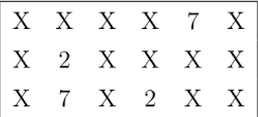
The solution adopted for the virtual environment is to virtualize the cards board using a textual representation. The game, now, can be played on the command line inserting the index of the card that the player wants to pick. A graphical view is proposed in the figure 6.1. In that, we can see how the cover cards are represented with a “X” and the image of the cards are replaced by number e.g.“2”.

X X X X 7 X X 2 X X X X X 7 X 2 X X

Figure 6.1: Command line version of the Memory game.

The program that is running behind the virtual board, is responsible to check the consistence of the board after each pick. This is possible verifying the following rules before displaying the selected card:

• If the selected card is not visible and there aren’t more then two cards turned over in the current turn, the selected card will be turned to show its image;

• If there are two cards turned over, the card will be checked. If both cards are equal, they stay visible on the board, otherwise both the cards are turned over again. In both the case a positive or negative reward is communicated to the agent.

The memory program is also responsible for the communication of the matching card position to the agent.

6.1.2

Virtual Agent

The virtual agent is not so di↵erent from the real one. The real agent is composed by the reinforcement learning algorithm, that perform the learning

6.1 Adaptation of Implementation 41 task, and Furhat, the physical body of the agent, that execs the actions in the environment.

The virtual agent is free from the physical body and directly communicate the selected action to the user. The simulated user will interpret the action and will react to it.

The communication are done with the exchanges of JSON packages like the one in the figure 6.2

action = {"speech" : 4, "facial" : 0, "head" : 5, "gaze" : 0} Figure 6.2: Example of virtual action.

6.1.3

Fictional User

To combine the policies we need policies generated from di↵erent users. For this purpose, using the techniques of the Personas [Schulz and Fu-glerud(2012)], we have generated a set of virtual users that di↵er for the value of the following features: a) Focus b) Memory c) Hearing and d) Sight.

The fictional users, defined in that way, are composed by two modules. The first is a simple intelligence that manage the selection of the cards and the second has the role of understand the suggestions provided by the agent.

The personas generated for the simulations are listed in Appendix A. User Behavior

The virtual user follows some really simple dynamics. His behavior can di↵er on the base of the card that he has to pick. When he has to select the first card, he checks whether he remembers the positions of two cards that make up a pair. If this happens the user will select one of the two cards, otherwise he will take a random card from the board excluding the cards that he already knows.

42 6. Virtual Simulation The selection of the second card is a bit more complicated because we need to simulate a reaction at the suggestions that is as realistic as possible. First of all the user checks for the presence of the matching card in his memory. If he doesn’t remember it, he will select a card following the suggestions of the agent in the limit of its features.

The suggestions are interpreted by the user in order to reduce the number of possible cards. Depending on the features of the user the action can be completely or partially ignored.

User Skill Translation

For each persona the features represented in the radar chart, with value included in the range 1 to 6, are converted to value understandable from the system.

The simulated user considers the actions performed by the agent with a probability of p, where

p = (focus 1)_{⇤ 0.2.} (6.1) User with low level of focus have a propensity to ignore the suggestions of the robot.

The memory feature is used to indicate the number of cards that the user can remember. These are equal to

m = memory + 1 (6.2) where the minimal possible result is 2 equivalent to a pair, the last seen.

The other two features are used to encode the impairment of the user. A user hears the speech suggestions with a probability of q, where

q = (hearing 1)_{⇤ 0.2.} (6.3) Users with a value equal to 1 are considered deaf, while users with a hearing value of 4 have just the 60% of probabilities to hear the suggestions.

The mapping of the sight is a bit di↵erent. It is performed following the information in the table 6.1. Each level encode the suggestion family that the user is able to perceive.

6.1 Adaptation of Implementation 43 Value User classification Perceived suggestions

6 Normal viewer Head movement, Facial expression, Gaze 5 Normal viewer Head movement, Facial expression, Gaze 4 Astigmatic Head movement, Facial expression 3 Myopic Head movement, Facial expression 2 Partially-sighted Head movement

1 Blind Nothing

Table 6.1: Sight mapping. User Memory Management

The user can remember only a limited number of cards that, in the worst case, is equal to 2. The discovered cards are added in the memory only after the end of the turn. This choice yields to a situation where the user, during a turn, knows all the cards that are showed on the board plus the cards in his memory. When the turn is over, and a pair is not discover, the picked cards are added to the memory. The memory can’t include pairs already discovered, because this will lock the card selection algorithm of the fictional user, so in the case that a pair already discovered is in the memory, it will be removed. When the memory is full and there is no space to store a new card, the oldest card in the memory will leave space for the new one.

Interpreter

This module is responsible for the interpretation of the actions performed by the agent. It takes the performed action and in the respect of the user features, return a set of cards where the user will randomly pick the next.

First we have to introduce the no informations set (NIS), a set composed of all the covered cards on the board less the cards remembered by the user. The function starts checking p to understand if the action has to be considered or ignored by the virtual user. In the case that the action is ignored the next card will be chosen in the NIS and no reward is given to

44 6. Virtual Simulation the agent in this turn. In the opposite case, when the fictional user doesn’t remember the card and decides to follow the suggestion, the intersection of the sets of cards derived from each suggestion that compose the action is returned to the main module of the user.

How are the sets of cards of each suggestion family made? To start a NIS is associated to each of them. The interpreter function checks the action received from the agent in each of its parts. These contain codes that are associated to virtual actions (fig 6.3) and a relative interpretation that will reduce the sets size of each suggestion set. If the final set is empty, because of inconsistent suggestions in the same action, a NIS is returned and a punishment of -3 is given to the agent.

The interpreter also gives an additional reward, equal to _{#(final set)}1 , to incentivize the use of specific suggestions and speed up the learning.

action = {"speech" : 4, "facial" : 0, "head" : 4, "gaze" : 0} Figure 6.3: Example of inconsistent action.

In the figure 6.3 we can see an example of inconsistent action due to the incompatibility of the speech and head suggestions. The voice is saying “Maybe down” while the head is pointing up. The resulting set of possible cards will be empty.

The interpretation of each suggestion are listed and explained in the Ap-pendix B.

6.2

Procedure

The simulation has been performed on all the generated fictional users. All of them are used to train a set of policies using both the learning

algo-6.3 Results 45 rithm1_{. For each algorithm the user has played 10 games composed of 500}

rounds. Each game generates a policy that improve after every turn2 _{of the}

rounds, where a round is composed by all the turns required to find all the pairs.

The training of each policy starts with the ✏ factor, responsible for the exploration, set to 0.9 that make the initial selection of the actions totally random ignoring the actions in the policy. Every 50 rounds, a tenth of game, the ✏ is decreased of 0.1 until it reaches the minimum value of 0.1. We are not interested in the initial value of , because the estimate of the optimal future value is always equal to 0. In Q-learning is also initialized the learning factor ↵. It start from a value of 0.5 and is decrease every 50 rounds of 0.05. When the policies of each user has been generated and collected, the policies combination algorithm can be tested. The policies of each user are stored in separate folder. Knowing the path of the users policies folders, the algorithm automatically extract the users information from the comparison of the policies and randomly selects a policy from each user, that is addressed to generate the final merged policy.

Di↵erent merged policies has been generated for di↵erent subset of users. Their goodness has been tested via multiple executions of a round in which a user, of the users set in cause, is assisted from a rule based agent that follow the merged policy.

6.3

Results

We will now see the results of the di↵erent step of the simulation. Not all the results are reported, but only the most significant for the understanding of the problem.

The first important results is that all the simulations where we have

1_{Online Q-learning and online LSPI}

46 6. Virtual Simulation generated the policies using online Q-learning have converged to an optimal solution in the selected number of rounds. This result has not been reached by the simulation that were running online LSPI.

An important result is the distribution of the number of picks used by the user to complete the single round. This number is expected to decrease during the simulation, but sometimes we can have di↵erent evolution due to the e↵cts of the features. In the figure 6.4 are shown the learning progress of di↵erent users. The x axis reports the number of the round, while the y axis represents the number of picks per round. Each graph highlights the e↵ect of a feature in the learning process.

With the policies obtained from the Q-learning algorithm is possible to extract the users information. The second results of the experiment are a comparison of the information extracted and the original features of the users and are reported in the figure 6.5. The figure is composed of two columns. On the left side we have the information extracted from the policies, while on the right are shown the graphical representations of the features.

Extracted the user information, the next step is the combination of the policies. The figure 6.6 gives a visual representation of the users policies. Each graph contains three policies. The two, without label, are the policies used for the combination while the one with the blue cross is the merged policy. On the axis are represented the code that identifies the states and the code of the composite actions.

6.3 Results 47

(a) Memory

(b) Focus

(c) Sight vs Hearing