1D transient simulation and fuel injection control of a turbocharged Diesel engine

(1)

School of Industrial and Information Engineering

Master of Science in Mechanical Engineering

1D TRANSIENT SIMULATION AND FUEL INJECTION

CONTROL OF A TURBOCHARGED DIESEL ENGINE

Supervisor: Prof. Gianluca D’Errico Thesis advisor: Prof. Tarcisio Cerri

Master’s thesis of:

Daniyal Altaf Baloch

Student ID: 882521

(2)

(3)

Astratto

Lo scopo di questa tesi è l'analisi delle mappe del motore e la simulazione transitoria 1D del motore diesel turbocompresso NEF6 sviluppato da FPT (Fiat Powertrain Technologies) per gli autobus.

Le simulazioni richieste per l'analisi sono eseguite su Gasdyn - un software di simulazione del motore monodimensionale sviluppato dal gruppo ICE del Dipartimento di Energia del Politecnico di Milano e ora concesso in licenza da Exothermia (leader mondiale nello sviluppo e nell'applicazione di strumenti software per il post-trattamento automobilistico simulazioni di sistema).

Il motore proposto è un motore turbo 6 cilindri con accensione a compressione.

La tesi incorpora la simulazione di indici di prestazione chiave del motore rispetto ai dati sperimentali. Oltre al modello base, viene applicato un controllo sulla pressione di sovralimentazione e sulla massa iniettata di carburante che entra nella camera di combustione.

Sono state inoltre emulate mappe dei motori statici che comportano carichi operativi diversi per entrambe le strategie di controllo e sono riportati gli errori relativi degli indici di

prestazione rispetto ai dati sperimentali. Tutti questi risultati vengono post elaborati in MS Excel per consentire una panoramica ampia e completa dei risultati.

Questa analisi ha aiutato a identificare diversi problemi per i motori CI in Gasdyn e in questo modo ha permesso di regolare e migliorare continuamente il software.

Principalmente, il controllo su BMEP attuando la massa di carburante iniettata viene studiato in questa tesi.

Infine, viene eseguita un'analisi transitoria del ciclo di guida del bus BSC per un modello di veicolo per valutare il consumo di carburante. La valutazione viene effettuata considerando il veicolo come massa in punti e incorporando le forze del motore, dello pneumatico, della trasmissione e della resistenza per calcolare il consumo di carburante.

(4)

Abstract

The aim of this thesis is the analysis of engine maps and 1D transient simulation of the NEF6 turbocharged diesel engine that is developed by FPT (Fiat Powertrain Technologies) for buses.

The simulations required for the analysis are performed on Gasdyn – a one-dimensional engine simulation software developed by ICE group of the Department of Energy at

Politecnico di Milano and now licensed by Exothermia (world leader in the development and application of software tools for automotive aftertreatment system simulations).

The proposed engine is a compression ignition 6-cylinder turbocharged engine. The thesis incorporates the simulation of key performance indices of the engine in

comparison with the experimental data. In addition to the base model, a control is applied on the boost pressure and the injected mass of fuel entering the combustion chamber.

Static engine maps entailing different operating loads have also been emulated for both control strategies and the relative errors of the performance indices with respect to the experimental data are reported. All these results are post processed in MS Excel to allow a broad and comprehensive overview of the results.

This analysis helped in identifying different issues for CI engines in Gasdyn and in this way made it possible to continuously adjust and improve the software.

Mainly, the control on BMEP by actuating the injected fuel mass is investigated in this thesis. Finally, a BSC bus driving cycle transient analysis is performed for a model vehicle to

evaluate the fuel consumption. The evaluation is done by considering the vehicle as point mass and incorporating the engine, tyre, transmission and resistance forces to calculate the fuel consumption.

(5)

List of Figures

Figure 1-1 Finite 1D control volume ... 3

Figure 2-1 Engine representation (Right) ... 9

Figure 2-2 Engine representation (Left) ... 9

Figure 2-3 GT-power model schematic ... 10

Figure 2-4 Gasdyn model schematic... 11

Figure 2-5 Duct object discretization ... 12

Figure 2-6 Duct object parameters in Gasdyn ... 13

Figure 2-7 GT-power FlowSplitGeneral equivalent representation in Gasdyn ... 13

Figure 2-8 Equivalent pipe junction model in CAD software ... 14

Figure 2-9 Turbocharger flow gases Schematic ... 15

Figure 2-10 Variable Geometry Turbine (VGT) working [2] ... 16

Figure 2-11 Twin Scroll Turbine ... 16

Figure 2-12 Compressor map parameters ... 17

Figure 2-13 Compressor Pressure ratio map ... 17

Figure 2-14 Compressor Efficiency map ... 18

Figure 2-15 Compressor Pressure ratio map (extended)... 18

Figure 2-16 Compressor Efficiency map (extended) ... 19

Figure 2-17 Turbine expansion ratio map ... 20

Figure 2-18 Turbine efficiency map ... 20

Figure 2-19 Clarification of SOI values to enter in Gasdyn ... 22

Figure 2-20 Valve timing diagram ... 22

Figure 2-21 Valves discharge flow coefficient as a function of L/D ... 23

Figure 2-22 Valves Effective flow area ... 23

Figure 2-23 DuctMatrix object in GasdynPre ... 24

Figure 2-24 Air mass flow rate ... 25

Figure 2-25 Temperature across intercooler ... 25

Figure 2-26 Temperature before compressor ... 25

Figure 2-27 Temperature after compressor ... 25

Figure 2-28 Pressure before compressor... 25

Figure 2-29 Pressure after compressor ... 25

Figure 2-30 Temperature before turbine ... 26

Figure 2-31Temperature after turbine ... 26

Figure 2-32 Pressure before turbine ... 26

Figure 2-33 Pressure after turbine... 26

Figure 3-1 BMEP comparison (Full load) ... 28

Figure 3-2 BMEP fitting with experimental data (Full load) ... 28

Figure 3-3 Modified Chen-Flynn coefficients in GasdynPre ... 29

Figure 3-4 Power comparison (Full load) ... 30

Figure 3-5 Torque comparison (Full load) ... 30

Figure 3-6 BSFC comparison (Full load) ... 31

Figure 3-7 Air mass flow comparison (Full load) ... 32

Figure 3-8 Injected fuel flow comparison (Full load) ... 32

Figure 3-9 AFR comparison (Full load) ... 32

Figure 3-10 Turbine speed comparison (Full load) ... 33

(8)

Figure 3-12 Turbocharger boost pressure convergence at 600 rpm (Full load) ... 33

Figure 3-13 Turbocharger boost pressure convergence at 1400 rpm (Full load) ... 34

Figure 3-14 Compressor map operating points (Full load) ... 34

Figure 4-1 BMEP relative error with changing PID gains ... 36

Figure 4-2 BMEP comparison (inj.Fuel control) ... 37

Figure 4-3 BMEP fitting (inj.Fuel control) ... 37

Figure 4-4 Brake Power comparison (inj.Fuel control) ... 37

Figure 4-5 Brake Torque comparison (inj.Fuel control) ... 37

Figure 4-6 BSFC comparison (inj.Fuel control) ... 37

Figure 4-7 Cylinder pressure comparison (inj.Fuel control) ... 38

Figure 4-8 Air mass flow comparison (inj.Fuel control) ... 38

Figure 4-9 Turbine speed comparison (inj.Fuel control) ... 38

Figure 4-10 NOx wet comparison (inj.Fuel control) ... 38

Figure 4-11 Boost pressure comparison (inj.Fuel control) ... 38

Figure 4-12 AFR comparison (inj.Fuel control) ... 38

Figure 5-1 Map generation utility in GasdynPre ... 39

Figure 5-2 BMEP map comparison ... 40

Figure 5-3 BSFC map comparison ... 40

Figure 5-4 NOx emissions map comparison ... 41

Figure 5-5 Peak cylinder pressure map comparison ... 41

Figure 5-6 BMEP error contour map (Case 1) ... 42

Figure 5-7 BMEP error contour map (Case 2)... 42

Figure 5-8 NOx error contour map (Case 1) ... 42

Figure 5-9 NOx error contour map (Case 2) ... 42

Figure 5-10 BSFC error contour map (Case 1) ... 42

Figure 5-11 BSFC error contour map (Case 2) ... 42

Figure 5-12 Peak Cylinder pressure error contour map (Case 1) ... 43

Figure 5-13 Peak Cylinder pressure error contour map (Case ) ... 43

Figure 5-14 Load vs BMEP error (Case 2) ... 43

Figure 5-15 Load vs Peak cylinder pressure error (Case 2) ... 43

Figure 5-16 Load vs BSFC error (Case 2) ... 44

Figure 5-17 Load vs NOx error (Case 2) ... 44

Figure 6-1 Torque and vehicle speed evolution from 0-100 km/h acceleration ... 48

Figure 6-2 Operating points for the acceleration test... 48

Figure 6-3 Bus brands for comparison... 49

Figure 6-4 Model of vehicle considered as point... 50

Figure 6-5 CI engine combustion efficiency isolines ... 52

Figure 6-6 Braunschweig driving cycle speed profile ... 53

Figure 6-7 Braunschweig driving cycle fuel consumption rate ... 53

Figure 6-8 Braunschweig driving cycle Cumulative fuel consumption ... 53

Figure 6-9 Braunschweig driving cycle Torque points... 54

Figure 6-10 Braunschweig driving cycle Brake power points... 54

(9)

List of Tables

Table 2-1 NEF6 Engine specifications (FPT) ... 9

Table 2-2 Comparison between GT-power and Gasdyn object elements ... 12

Table 2-3 Geometrical parameters of a FlowSplitGeneral element ... 14

Table 2-4 Turbine map parameters ... 19

Table 2-5 SOI and fuel mass fraction values at Full load ... 21

Table 3-1 PID gains for boost pressure control ... 27

Table 4-1 BMEP across the engine speed range ... 35

Table 4-2 Adaptive PID gains for fuel mass control ... 36

Table 6-1 Man's Lion City 12C specifications ... 45

Table 6-2 Tyre dimensions, Gearbox and Differential data ... 46

Table 6-3 Bus loading for acceleration test ... 46

Table 6-4 Vehicle transient panel in GasdynPre... 47

Table 6-5 Gear ratios and shifting time ... 47

Table 6-6 Bus driving cycles ... 49

Table 6-7 Bus brand A and B loading condition ... 49

Table 6-8 f0 (road influence coefficient) values for different surfaces ... 51

(10)

(11)

Introduction

A six-cylinder turbocharged diesel engine has been simulated using Gasdyn, a 1D engine systems simulation software. The results are then compared with the experimental data provided by FPT (Fiat Powertrain Technologies). This engine is designed for a bus and also been simulated on GT-power by the OEM. Initially, all the data was given as the GT-power model along with experimental test data for the ducts, auxiliaries, cylinders and turbocharger. In this thesis different performance parameters are evaluated to be compared with the data. In the following chapters, the modeling of the engine on Gasdyn, the comparison of results for full load and static maps, implementation of PID control on injected fuel and finally a transient vehicle analysis to determine fuel consumption for a model bus is presented. The chapters to follow can be outlined as below:

Chapter 1 The rudimentary theoretical knowledge on the working principle of a numerical software like Gasdyn to solve the complex phenomena occurring within the internal combustion engines is presented. It encapsulates the solving of conservation equations (Navier-Stokes) while adopting some assumptions.

Chapter 2 The modeling process of the engine system within the Gasdyn GUI is illustrated emphasizing the most important parameters to consider as well as some strategies to transform GT-power elements to Gasdyn where needed.

Chapter 3 Performance indices of an engine like BMEP, power, torque and BSFC for a full load operation are presented.

Chapter 4 PID control strategy on injected fuel mass apart from the PID control on boost pressure is analyzed and the effective results are compared.

Chapter 5 Static maps covering the entire engine speed and load spectrum are simulated and contour maps on percentage error relative to the experimental data are shown.

Chapter 6 A vehicle transient simulation for a model bus is emulated over a BSC – Braunschweig city bus driving cycle to calculate the fuel consumption.

(12)

GASDYN overview

1 GASDYN overview

Gas Dynamics or GASDYN is a one-dimensional engine simulator. In this thesis, all the simulated results are obtained through GASDYN and the complete procedure from start to finish is discussed comprehensively in the next chapter.

The solution to any fluid dynamic problem is obtained by finding the most crucial parameters of a flow that are pressure and velocity. Such a solution is obtained by solving the Navier-Stokes equation which is a combination of the conservation equations for mass, momentum and energy. For a simple flow problem like the one for a flow in a straight pipe, the solution can be found analytically and through empirical correlations. However, for complex

problems, analytical solutions are not available and hence must be solved numerically using computers.

In any numerical solver, the field through which the flow passes, is discretized into small volumes over which the pressure and velocity fields are evaluated. These small volumes of fluid when combined form the complete solution of the flow problem. Flow problems are, in reality, three dimensional, however, some careful assumptions ease them into one

dimensional problem which save a significant amount of computational effort.

Gasdyn, in a similar fashion, is a one-dimensional flow solver for entire internal combustion engine systems. In the following sections a brief overview of the governing equations and Gasdyn’ s approach to solution are introduced.

1.1 One-dimensional conservation equations

Gases flowing inside an entire IC engine system are subject to unsteadiness and compressibility. The flow is highly turbulent, and friction plays an important role. In addition, the gases flowing into different components cause the fluid to move through variable cross sections, temperatures and interacting pressures.

A 3D analysis would be in best consistency with a real flow cycle, but it would take significant computational power to solve numerically. Gasdyn, upon certain assumptions, solves the flow field in 1D in order to save time and predicts very close results quickly. This is the main advantage of such a code.

The Navier-Stokes equation entails: • Mass conservation equation • Momentum conservation equation • Energy conservation equation

(13)

GASDYN overview

Figure 1-1 Finite 1D control volume

Figure 1-1 represents a typical control volume of length 𝑑𝑥 with the states of a fluid 𝑝, 𝜌, 𝐹, 𝑢 entering and leaving the control volume.

Where the terms above are: 𝑝 Pressure

𝜌 Density

𝐹 Cross-sectional area 𝑢 Fluid velocity 𝜏_𝑤 Wall shear stress

1.1.1 Mass conservation equation

The difference between the mass flow rate leaving the control volume and the mass flow rate entering is equal to the rate of change in mass within the volume itself.

(𝜌 +𝜕𝜌 𝜕𝑥𝑑𝑥) (𝑢 + 𝜕𝑢 𝜕𝑥𝑑𝑥) (𝐹 + 𝜕𝐹 𝜕𝑥𝑑𝑥) − 𝜌𝑢𝐹 = − 𝜕 𝜕𝑡(𝜌𝐹𝑑𝑥)

Rearranging equation above and neglecting second order infinitesimals, it is obtained: 𝜕𝜌 𝜕𝑡 + 𝜌 𝜕𝑢 𝜕𝑥+ 𝑢 𝜕𝜌 𝜕𝑥+ 𝜌𝑢 𝐹 𝜕𝐹 𝜕𝑥 = 0

1.1.2 Momentum conservation equation

The sum of the pressure forces and the shear forces acting on the surface of the control volume is equal to the sum of the rate of change of momentum within the control volume and the net efflux of momentum out of it.

Pressure forces: 𝑝𝐹 − (𝑝 +𝜕𝑝 𝜕𝑥𝑑𝑥) (𝐹 + 𝜕𝐹 𝜕𝑥𝑑𝑥) + 𝑝 𝑑𝐹 𝑑𝑥𝑑𝑥 = − 𝜕(𝜌𝐹) 𝜕𝑥 𝑑𝑥 + 𝑝 𝑑𝐹 𝑑𝑥𝑑𝑥

(14)

GASDYN overview Shear stress (f is the friction factor):

𝜏𝑤 = 𝑓 ∙

1 2𝜌𝑢

2

The force applied on the lateral wall surface caused by friction: 𝐹_{𝑓𝑟𝑖𝑐𝑡𝑖𝑜𝑛} = −𝑓 ∙1

2𝜌𝑢

2_{∙ (𝜋𝐷𝑑𝑥)}

The rate of change of momentum in the volume: 𝜕

𝜕𝑡(𝜌𝑢𝐹𝑑𝑥) The net efflux of momentum from the control surface:

(𝜌 +𝜕𝜌 𝜕𝑥𝑑𝑥) (𝑢 + 𝜕𝑢 𝜕𝑥𝑑𝑥) 2 (𝐹 +𝜕𝐹 𝜕𝑥𝑑𝑥) − 𝜌𝑢 2_{𝐹 ≈}𝜕(𝜌𝑢 2_𝐹) 𝜕𝑥 𝑑𝑥

Considering the mass conservation equation, the momentum equation results to be as follows. 𝜕𝑢 𝜕𝑡 + 𝑢 𝜕𝜌 𝜕𝑥+ 1 𝜌 𝜕𝜌 𝜕𝑥+ 𝐺 = 0 G accounts for the viscosity.

𝐺 = 𝑓𝑢 2 2 𝑢 |𝑢| 4 𝐷

1.1.3 Energy conservation equation

Applying the First Law Thermodynamic to the control volume the conservation equation of energy is derived.

The conservation equation states that the difference between the heat transfer rate between fluid and pipe through the pipe walls and the mechanical work rate done by or on the fluid equals the sum of the variation in time of the total stagnation internal energy and the net flux of stagnation enthalpy across the control surface.

𝑄̇ − 𝐿̇ =𝜕𝐸0 𝜕𝑡 +

𝜕𝐻₀ 𝜕𝑥 𝑑𝑥

In order to obtain the final expression of the energy conservation equation it is necessary to better specify the single terms.

𝑄̇is the heat entering the control volume through the walls of the pipe. 𝑄̇ = 𝑞 ∙ 𝜌𝐹𝑑𝑥 + ∆𝐻𝑟𝑒𝑎𝑐𝑡𝑖𝑜𝑛𝐹𝑑𝑥

(15)

GASDYN overview q is the heat exchanged through the control volume per unit of mass and time; ∆𝐻_{𝑟𝑒𝑎𝑐𝑡𝑖𝑜𝑛} is the heat released per unit of time and volume by some chemical reactions occurring in the gas flow.

𝜕𝐸0

𝜕𝑡 is the variation in time of the total stagnation internal energy.

𝜕𝐸0

𝜕𝑡 =

𝜕(𝑒0𝜌𝐹𝑑𝑥)

𝜕𝑡 whereas 𝑒₀ is the specific stagnation energy.

𝑒₀ = 𝑒 +𝑢

2

𝜕𝐻0

𝜕𝑥 is the net flux of stagnation enthalpy through the control surface.

𝜕𝐻₀ 𝜕𝑥 =

𝜕(ℎ₀𝜌𝐹𝑢)

𝜕𝑥 𝑑𝑥

Where the specific stagnation enthalpy is: ℎ0 = 𝑒0+ 𝑝 𝜌= 𝑐𝑣𝑇 + 𝑝 𝜌+ 𝑢2 2

Finally, introducing a as the speed of sound, considering mass and momentum equations, the expression of the energy conservation equation results:

𝜕𝜌 𝜕𝑡 + 𝑢 𝜕𝜌 𝜕𝑥− 𝑎 2₍𝜕𝜌 𝜕𝑡 + 𝑢 𝜕𝜌 𝜕𝑥) − (𝑘 − 1)𝜌(𝑞 + 𝑢𝐺) = 0 According to the hypothesis of perfect gas model, the speed of sound is given by:

𝑎 = √𝑘𝑅𝑇

Where T is the temperature, R is the universal gas constant and 𝑘 =𝑐𝑝

𝑐𝑣 .

1.1.4 Conservative form of conservation equations

The system made by conservation equations represents the hyperbolic problem written in non-conservative form. { 𝜕𝜌𝐹 𝜕𝑡 + 𝜕(𝜌𝑢𝐹) 𝜕𝑥 = 0 𝜕(𝜌𝑢𝐹) 𝜕𝑡 + 𝜕((𝜌𝑢2+ 𝑝)𝐹) 𝜕𝑥 − 𝑝 𝜕𝐹 𝜕𝑥+ 𝜌𝐺𝐹 = 0 𝜕(𝜌𝑒₀𝐹) 𝜕𝑡 + 𝜕(𝜌𝑢ℎ₀𝐹) 𝜕𝑥 − 𝜌𝑞𝐹 = 0

(16)

GASDYN overview

In order to simplify the resolution of the system, this can be written in conservative form and then expressed in matrix form.

In the conservative form the classical momentum equation is substituted by the impulse equation which is a linear combination of the mass and the momentum equations. It is possible to group some terms and create three vectors.

• Vector of conserved variables

𝑊̅ (𝑥, 𝑡) = [ 𝜌𝐹 𝜌𝐹 𝜌𝑒₀𝐹

]

These three variables are independent, they vary with x and t and their fluxes are conserved along the shockwave.

• Vector of conserved variable fluxes

𝐹̅(𝑊̅ ) = [

𝜌𝑢𝐹 (𝜌𝑢2_{+ 𝑝)𝐹}

𝜌𝑢ℎ₀𝐹 ]

Mass, impulse and stagnation enthalpy fluxes are conserved through the boundaries. • Vector of source terms

𝐶̅(𝑊̅ ) = [ 0 −𝑝𝑑𝐹 𝑑𝑥 0 ] + [ 0 𝜌𝐺𝐹 −𝜌𝑞𝐹 ]

It is given by the contributes of two vectors. The first vector contains the source terms due to the variation of the cross section along the duct; the second contains the source terms due to the friction between the fluid and the walls and to the heat exchange with the fluid.

Finally, the conservation equations can be written in the compact form: 𝜕𝑊̅ (𝑥, 𝑡)

𝜕𝑡 +

𝜕𝐹̅(𝑊̅ )

𝜕𝑥 + 𝐶̅(𝑊̅ ) = 0

Now, the system has three equations in four unknowns (𝑝, 𝑢, 𝑒, 𝜌), so a fourth equation is required in order to achieve a solution.

This additional equation has to be found in the fluid characteristics.

It can be adopted the ideal gas model with constant specific heat or the mixture of ideal gas model.

In the case of gases in engine manifolds and cylinders the ideal gas model is, usually, adopted and the system is closed by the state equation of ideal gas:

(17)

GASDYN overview 𝑝

𝜌 = 𝑅𝑇

Actually, this equation introduces the gas temperature T as a new variable, but for an ideal gas internal energy and enthalpy are both functions of the temperature. So, in the system the equations reported below have to be added.

𝑒 = 𝑒(𝑇) ℎ = 𝑒(𝑇) + 𝑅𝑇

In case of perfect gas, specific heat at constant volume 𝑐_𝑣 and pressure 𝑐_𝑝 can be introduced and the previous equations become:

𝑒 = 𝑐_𝑣𝑇 ℎ = 𝑐_𝑝𝑇

In conclusion, including equations of internal energy and enthalpy to the system, a closed set of equations is obtained, characterized by six independent equations in six unknowns

(𝑝, 𝑢, 𝑒, 𝜌, ℎ, 𝑇). The solution of this system coupled with the proper boundary conditions, determines the flow conditions in any section of the duct.

1.2 Numerical methods

In general, it is not possible to obtain analytical solutions for the set of partial differential equations introduced above, so numerical solutions are required.

In order to determine the variation of all the physical parameters of the fluid in the pipe for each spatial and time condition, it is necessary to split the continuum fluid mass in a discrete number of smaller elements forming a grid. Then, the governing equations have to be

discretized becoming algebraic equations that a computer is able to solve. The solution of these equations is a duty of the numerical method applied.

For a long time, the Method of characteristic has been used, which has a first-order accuracy in space and time. But it gives problems in presence of discontinuities.

So, later on, this method has been substituted by the Shock-capturing method.

1.2.1 Shock-capturing numerical method

The numerical solution of the conservation equations written in the conservative form is computed by Gasdyn using the Shock-capturing method in each internal node of the pipes. Along the pipes the fluid is subjected to changes in temperature, pressure, chemical

(18)

GASDYN overview Shock waves cause contact discontinuities which lead to discontinuities in the numerical solution too. The Shock-capturing method is able to solve this problem and give an accurate solution. It is based on the application in each node of the same finite differences scheme, in order to represent the spatial derivative terms.

It is applied to the conservation equation written in compact matrix form X and has a second order accuracy in the space-time domain.

Two adjustments have to be introduced:

▪ the vector 𝑊(𝑥, 𝑡) is replaced by 𝑊_𝑖𝑛_{, meaning 𝑊(𝑖𝛥𝑥, 𝑛𝛥𝑡), where the indices i and}

n are referred to space and time. ▪ the source vectors are deleted. in this way, the Equation X becomes:

𝜕𝑊̅ 𝜕𝑡 +

𝜕𝐹̅(𝑊̅ )

𝜕𝑥 = 0

Integrating X in a grid divided in 𝛥𝑥 and 𝛥𝑡 meshes, Y is obtained

∫ ∫ 𝜕𝑊̅ 𝜕𝑡 + 𝜕𝐹̅(𝑊̅ ) 𝜕𝑥 𝑑𝑥𝑑𝑡 = 0 𝑥+∆𝑥 𝑥 𝑡+∆𝑡 𝑡 (𝑊̅_𝑖𝑛+1− 𝑊̅_𝑖𝑛)∆𝑥 + (𝐹̅ 𝑖+1₂ 𝑛+1_{− 𝐹̅} 𝑖−1₂ 𝑛 _{) ∆𝑡 = 0}

The space discretization for 𝐹̅ is central differencing that is why we have ½ on each side of the calculation point "𝑖".

In this way, the aforementioned problem linked to the derivability condition of Euler Equations is avoided, because the integral form is able to detect the contact discontinuities without knowing their location.

Rearranging the expression above we can get another formulation which represents the discretization of continuous that has to be implemented in the method at finite differences.

(𝑊̅_𝑖𝑛+1− 𝑊̅_𝑖𝑛) ∆𝑡 + (𝐹̅ 𝑖+1₂ 𝑛+1_{− 𝐹̅} 𝑖−1₂ 𝑛 ₎ ∆𝑥 Summing the differences along 𝑥:

∆𝑥 ∑ 𝑊̅_𝑖𝑛+1 𝑖,𝑚𝑎𝑥 𝑖,𝑚𝑖𝑛 = ∆𝑥 ∑ 𝑊̅_𝑖𝑛 𝑖,𝑚𝑎𝑥 𝑖,𝑚𝑖𝑛 + ∆𝑡 (𝐹̅ 𝑖+1₂ 𝑛+1_{− 𝐹̅} 𝑖−1₂ 𝑛 ₎

This expression above means that the total mass, momentum and energy at time n+1 equals the sum of the total mass, momentum and energy at time n plus the fluxes through the ends of the duct. It represents a conservative discretization scheme.

In particular, Gasdyn adopts Lax-Wendroff and MacCormack Shock-capturing technics, but their detailed description is behind the aim of this thesis.

(19)

Engine model

2 Engine model

2.1 Engine data

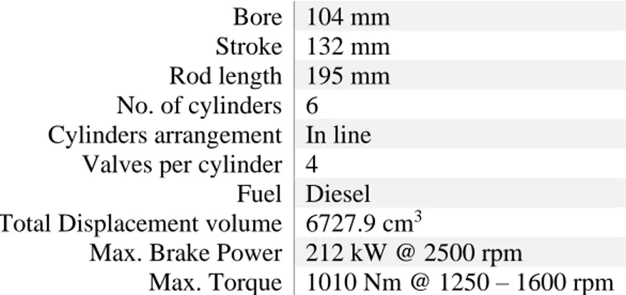
The model engine is a 6-cylinder turbocharged diesel engine with the specifications in Table 2-1. It has been developed by Fiat Powertrain Technologies (FPT) for a bus.

Bore 104 mm Stroke 132 mm Rod length 195 mm No. of cylinders 6 Cylinders arrangement In line

Valves per cylinder 4 Fuel Diesel Total Displacement volume 6727.9 cm3

Max. Brake Power 212 kW @ 2500 rpm

Max. Torque 1010 Nm @ 1250 – 1600 rpm

Table 2-1 NEF6 Engine specifications (FPT)

The engine model by FPT was created on GT-power – a widely used engine simulation and testing software in the automotive industry. The GT-power model has been recreated in GASDYN based on the complete data of engine, piping, turbocharger, intercooler and all interconnected components. Using such dimensions and specifications, the same engine was modeled in GASDYN as shown in Figure 2-4. In the next sections, a concise guide to this modeling process has been elaborated.

As in our case, usually the data is provided as *.dat file which, though contains most of the information, requires searching for the data inside the file unlike what you find in MS Excel worksheets. So, as we proceed with the following sections, some important keywords that help in the search will be discussed briefly.

(20)

Engine model

The GT-power configuration for the engine is shown. Using this model as reference, the Gasdyn model will be created. The technical data for all the components of this engine system is provided by the manufacturer.

(21)

Engine model

Figure 2-4 Gasdyn model schematic

This model is created in the preprocessor module of Gasdyn called GasdynPre. Different components are connected together to form a complete system. It is very important in the initial design stages to model the system as close to the original in order to get consistent results comparable with the experimental data. The pipe lengths, cylinder geometry, turbocharger maps and all initial data required to successfully run a simulation should be checked and confirmed.

All the regions where an output is required to check the parameters like pressure, temperature and mass flow should be assigned the output sensor using the output checkbox inside the respective object panel.

(22)

Engine model

2.2 Gasdyn Pre GUI / Modelling process

The initial step is to understand the software’s Graphical User interface and through some example models provided through the software’s built-in documentation. As can be seen in the GT-Power model, it contains different joining components like 90-degree elbows, orifices and splitters. In Table 2-2 we find the alternatives (objects) in Gasdyn of such GT-power components.

GT-power Gasdyn

PipeRound element Duct

FlowsplitGeneral Elements Junction

FlowSplitTRight Elements Multipipe junction

Table 2-2 Comparison between GT-power and Gasdyn object elements

The data provided by FPT covers the following data types: • Inlet/Outlet pipe diameters,

• Wall temperatures,

• Measured performance parameters (Power, Torque, BMEP, BSFC etc.), • Measured emissions (NOx, COx)

• Pressures and temperatures downstream/upstream of compressor & turbine. • Valve timings

• Fuel injector nozzle diameter and no. of holes.

As seen in the GT-power model in Figure 2-3. Each component has been labelled and hence can be referred to during search in the *.dat file. The preliminary task is to align the different pipe segments and components similar to the GT-power model.

2.2.1 Duct Object

In Gasdyn, a pipe element can be defined by diameter, length, wall temperature,

discretization length and radius of curvature in case of a curved duct. The discretization length is basically the unit space dimension for the numerical model to solve the velocity and pressure fields through the conservation equations. See Figure 2-5.

Two illustrative figures from the Duct object tab are shown below:

(23)

Engine model

Figure 2-6 Duct object parameters in Gasdyn

2.2.2 Junction object

The definition of a flowSplitGeneral element (junction object in Gasdyn), along with other parameters, requires the need to calculate the volume of the junction. For this purpose, we can use any 3D CAD software to join pipe elements and using the built-in tools to calculate the volume. I have used SolidWorks and the model is shown in Figure 2-8. The model is based on three cylindrical sections whose volume sum upto the one given by data.

Figure 2-7 GT-power FlowSplitGeneral equivalent representation in Gasdyn

The data from a GT-power model, contains the volume and angular positions of the junction legs with respect to three coordinate axes x, y and z. An illustrative figure below shows the angular positions of a flowSplitGeneral element, the data for which is tabulated as:

(24)

Engine model FlowsplitGeneral Elements

Name Volume Surface Area Boundary Connections Dependent

Parts in Map

mm3 mm2

Exhaust-Manifold1 73000 def Boundary Number 1 2 3 147 , 155

Angle wrt X-axis (3D) -135 -180 0

Angle wrt Y-axis (3D) -45 -90 90

Angle wrt Z-axis (3D) 90 90 90

Characteristic Length mm 37 68 68

Expansion Diameter mm 37 37 37

Table 2-3 Geometrical parameters of a FlowSplitGeneral element

Figure 2-8 Equivalent pipe junction model in CAD software

When defining a junction object in Gasdyn, the junction will be connected to three duct objects with lengths and diameters according to Table 2-3 in order to achieve the same volume as provided in data.

The characteristic length defines the distance the flow entering the boundary will travel before crossing another boundary or impacting a surface [1].

Boundary 2

Boundary 3

(25)

Engine model

2.2.3 Turbine and compressor

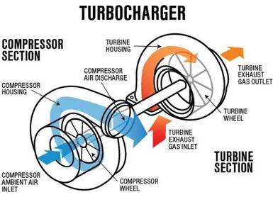
A turbocharger is a turbine and compressor as a single unit that increases the power output of an engine while keeping the same volume displacement of the engine. The compressor and the turbine rotate on a single shaft. The hot exhaust gases coming out of the cylinder pass through the turbine, the rotation of which rotates the compressor for which the intake is the ambient air.

The compressed air downstream of the compressor goes to the combustion chamber. This increase in the charge volume increases the volumetric efficiency of the engine and also the power output. Maintaining the same displacement volume means limiting the pollutant emissions.

Figure 2-9 Turbocharger flow gases Schematic

The pressure of the compressed air is also termed as “Boost pressure”. The boost pressure also needs to be controlled to avoid too much pressure increase which makes the engine susceptible to knocking. In order to limit the boost pressure, the exhaust gas headed towards the turbine is partially deviated and then joined back downstream of the turbine.

The decrease of flow rate of exhaust gases passing through the turbine decreases the turbine work and hence the shaft speed and consequently the boost pressure downstream of

compressor.

Such a control is materialized using a variable geometry turbine (VGT) or a waste-gate valve. A VGT consists of internal inlet guide vanes that are pivoted to rotate according to required flow rate. A waste-gate valve is a valve external to the turbine housing and opens and closes according to the pressure of incoming exhaust gases.

(26)

Engine model In Gasdyn Pre, we have the option for both; in case of a VGT, the turbine maps are defined over different VGT openings, meanwhile for a waste-gate valve, the user defines the gate opening as a percentage value over the entire speed range. Since in this thesis, a PID controller is acting on the waste-gate valve, it is not needed to define the opening values manually.

Figure 2-10 Variable Geometry Turbine (VGT) working [2]

Furthermore, the turbine used is a twin-scroll type i.e. having two inlets to the turbine. Each inlet/scroll accepts the exhaust from three cylinders.

Figure 2-11 Twin Scroll Turbine

The operating range of a turbocharger is defined by characteristic maps of the compressor and turbine. The maps are defined over reduced or non-dimensional terms and hence such maps can be applied to different sizes and operating range of turbochargers based on the theory of similitude.

The parameters to define the maps were provided by FPT. Using the Gasdyn modules “Turbine preprocessor” and “Compressor preprocessor” the characteristic curves are implemented in Gasdyn for the objects Compressor and Turbine .

(27)

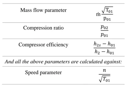
Engine model 2.2.3.1 Compressor map

Parameters to define the compressor curve are: Mass flow parameter

ṁ√T01 p₀₁ Compression ratio 𝑝02 𝑝₀₁ Compressor efficiency ℎ2𝑠− ℎ01 ℎ₂ − ℎ₀₁ And all the above parameters are calculated against:

Speed parameter 𝑛

√𝑇01

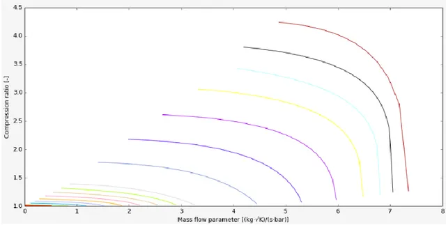
Figure 2-12 Compressor map parameters

The data for the compressor parameters given by FPT were absolute values i.e. speed [rpm] and mass flow rate [kg/s]. So, preprocessing of data was necessary using Compressor preprocessor module inside Gasdyn Pre.

(28)

Engine model

Figure 2-14 Compressor Efficiency map

For operations at low engine speeds below 800 RPM, these curves do not satisfy the performance requirement and hence the map was extended for correct working at lower engine speeds. The extended maps are shown in Figures 2-15 and 2-16.

Using the extended maps, the model was able to emulate the achievement of target boost pressures at low engine speeds and even more critical at low loads of these low speeds. However, the speeds at upper end of the range did not pose any problem because they operated in the real functioning zone of the maps originally provided by the manufacturer.

(29)

Engine model

Figure 2-16 Compressor Efficiency map (extended)

2.2.3.2 Turbine map

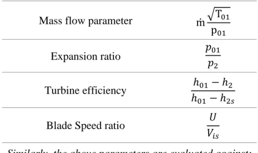
Quite similar to that of the compressor, the parameters to define the turbine curve are:

Mass flow parameter _ṁ√T01

p01

Expansion ratio 𝑝01

𝑝₂ Turbine efficiency ℎ01− ℎ2

ℎ₀₁− ℎ_2𝑠

Blade Speed ratio 𝑈

𝑉_𝑖𝑠

Similarly, the above parameters are evaluated against:

Speed parameter 𝑛

√𝑇01

(30)

Engine model

Figure 2-17 Turbine expansion ratio map

(31)

Engine model

2.2.4 Cylinder and Valves

The combustion model adopted is the Double-Wiebe function. This model requires the following parameters:

• Injected mass of fuel • Injection pressure of fuel

• Weight and Air-coefficients factor • No. of injections per cycle

• Injected mass fraction of fuel • SOI (Start of Injection) values

The experimental data for the above-mentioned parameters is tabulated below: Main fuel injection (M1) Post fuel injection (P1) engine speed [rpm] c.a. delay [deg] SOI [bTDC]

mass fraction SOI [bTDC]

mass fraction Fuel injected [kg/cyl/cycle] 600 1.368 -3.215530007 0.966790917 17.23950008 0.033209083 5.96376E-05 650 1.482 -2.602609999 0.970598224 19.11360013 0.029401776 6.80231E-05 800 1.824 -2.829249977 0.976177884 19.19309938 0.023822116 8.39556E-05 1000 2.28 -2.28774677 0.975639868 19.75009987 0.024360132 0.000108616 1100 2.508 0.18017997 0.976404068 22.79199924 0.023595932 0.000112808 1250 2.85 1.361850166 1 0 0 0.000115357 1400 3.192 2.127779873 1 0 0 0.0001144 1500 3.42 2.908969955 1 0 0 0.000113093 1600 3.648 3.691149952 1 0 0 0.000113023 1700 3.876 4.344450401 1 0 0 0.000111598 1800 4.104 4.446740242 1 0 0 0.00011139 1900 4.332 4.21536042 1 0 0 0.000111154 1950 4.446 4.035450081 1 0 0 0.000110988 2000 4.56 3.874539795 1 0 0 0.000110784 2200 5.016 3.472769531 1 0 0 0.000109941 2300 5.244 3.569010216 1 0 0 0.000107566 2400 5.472 3.957650307 1 0 0 0.000104469 2500 5.7 4.392499733 1 0 0 0.000101072

Table 2-5 SOI and fuel mass fraction values at Full load

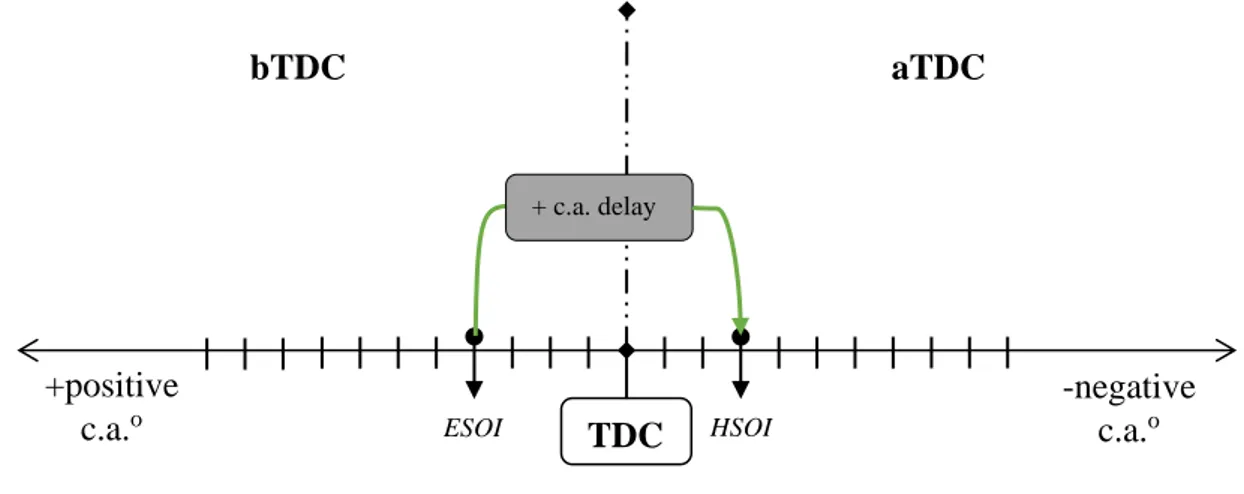
The SOI (Start of Injection) values initially provided by FPT were the electronic SOI values while the SOI to be inserted in Gasdyn should be, by default, the hydraulic SOI values. For this purpose, a delay of 380µs was implemented to calculate the hydraulic SOI as:

(32)

Engine model 𝑆𝑂𝐼_{ℎ𝑦𝑑𝑟𝑎𝑢𝑙𝑖𝑐} = 𝑆𝑂𝐼_{𝑒𝑙𝑒𝑐𝑡𝑟𝑜𝑛𝑖𝑐}+ (𝑐. 𝑎. 𝑑𝑒𝑙𝑎𝑦) where, 𝑐. 𝑎. 𝑑𝑒𝑙𝑎𝑦 = 360 [ 𝑑𝑒𝑔 𝑟𝑜𝑢𝑛𝑑] × 𝑁 [ 𝑟𝑜𝑢𝑛𝑑 𝑚𝑖𝑛 ] × 1 60 [_{𝑚𝑖𝑛]}𝑠𝑒𝑐 × 380 ∙ 10 −6_{[𝑠𝑒𝑐]}

It is very important to note that the SOI values inserted in Gasdyn are bTDC1_{i.e. bTDC}

values should be positive (+). So, if any value is negative, that means it is aTDC2.

Figure 2-19 Clarification of SOI values to enter in Gasdyn

The cylinder has two inlet and two exhaust valves with reference diameters of 30.6 mm each. The valve timing diagram, discharge flow coefficient and effective flow area graphs are shown below

Figure 2-20 Valve timing diagram

1_{before Top Dead Center}

2_{after Top Dead Center}

bTDC aTDC

-negative c.a.o

+positive

c.a.o ESOI HSOI

+ c.a. delay

(33)

Engine model

Figure 2-21 Valves discharge flow coefficient as a function of L/D

Figure 2-22 Valves Effective flow area 0 0.1 0.2 0.3 0.4 0.5 0.6 0 0.05 0.1 0.15 0.2 0.25 0.3 0.35 0.4 0.45 Flo w co ef f [-] L/D

Discharge Flow coeff.

Inlet Exhaust -50 0 50 100 150 200 250 300 350 400 100 150 200 250 300 350 400 450 500 550 600 E ff ec tiv e flo w ar ea [ m m 2 ]

Crank angle [deg]

Effective flow area

(34)

Engine model

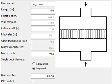
2.2.5 Intercooler

The compression of intake air causes its temperature to increase. This rise in temperature of the air causes its density to decrease which penalizes the volumetric efficiency. Therefore, in order to decrease the temperature of the compressed air, an intercooler is installed

downstream of the compressor.

The intercooler is effectively a heat exchanger the cools down the high-pressure intake air before discharging it into the intake manifold. The object for air intercoolers is “DuctMatrix” in GasdynPre shown in Figure 2-23.

The main parameters to define inside the DuctMatrix object panel are: • Total length

• Number of ducts • Duct diameter

Figure 2-23 DuctMatrix object in GasdynPre

2.3 Model validation

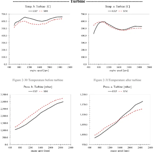
The results of any simulation can be as reliable as the model itself. Therefore, an initial run is essential to validate the model. Since the geometry of the entire engine system is based on the GT-power model, the geometry created in Gasdyn should satisfy those requirements in terms of pressure, temperature and air flow rates upstream and downstream of the compressor, turbine and intercooler.

In the following figures, the validity of our model is considered very satisfactory since the values closely match with those of the experiments.

(35)

Engine model

Figure 2-24 Air mass flow rate Figure 2-25 Temperature across intercooler --- Compressor ---

Figure 2-26 Temperature before compressor Figure 2-27 Temperature after compressor

(36)

Engine model

--- Turbine ---

Figure 2-30 Temperature before turbine Figure 2-31Temperature after turbine

Figure 2-32 Pressure before turbine Figure 2-33 Pressure after turbine

2.3.1 Ready to run

The regime of engine speed at which the performance indices have to be simulated is defined inside the General tab. The engine regime covers 600 to 2500 rpm.

Upon the complete setup and compilation of the model parameters, the simulation was run, and results viewed through the “Gasdyn Post” module. Not all results can be effectively obtained from the Gasdyn Post module and hence within the compiled folder/working directory, the respective files with *.axi extension can be replaced with extension *.csv and easily viewed in MS Excel program.

(37)

Full load results

3 Full load results

Load in a compression ignition engine is controlled by the amount of fuel injected into the cylinder unlike the Spark ignition engine where load is controlled by the throttle valve. In this chapter, the comparison of the different performance parameters between the experimental data and simulated results is presented as normalized values i.e.

𝑠𝑖𝑚𝑢𝑙𝑎𝑡𝑒𝑑 𝑣𝑎𝑙𝑢𝑒

𝑚𝑎𝑥𝑖𝑚𝑢𝑚 𝑜𝑓 𝑒𝑥𝑝𝑒𝑟𝑖𝑚𝑒𝑛𝑡𝑎𝑙 𝑣𝑎𝑙𝑢𝑒𝑠 The performance indices that are compared are:

• Brake Power • Brake Torque

• Brake Mean Effective Pressure (BMEP) • Break Specific Fuel Consumption (BSFC) • Peak cylinder pressure

• NOx Emissions • Turbocharger speed

The following comparisons refer to the Gasdyn model with the implementation of a single control on the boost pressure with following PID parameters3:

Target parameter Boost pressure

Actuated parameter Waste gate valve opening KP -0.6

KI -8.0

KD 0

Table 3-1 PID gains for boost pressure control

3.1 Performance indices

BMEP is one of the main performance parameters to compare engines. It is the effective work per unit cycle per unit volume displaced by the engine. It is defined as:

𝐵𝑀𝐸𝑃 = 𝜂_𝑏∙ 𝜆_𝑣∙𝜌𝑎

𝛼 ∙ 𝐿𝐻𝑉 In which the terms are:

𝜂𝑏 engine brake efficiency

𝜆𝑣 engine volumetric efficiency

𝜌_𝑎 density of air 𝛼 air to fuel ratio

𝐿𝐻𝑉 Lower Heating Value of fuel

(38)

Full load results BMEP is also derived from the difference of the frictional from the indicated mean effective pressure.

𝐵𝑀𝐸𝑃 = 𝐼𝑀𝐸𝑃 − 𝐹𝑀𝐸𝑃

Figure 3-1 BMEP comparison (Full load)

Figure 3-2 BMEP fitting with experimental data (Full load)

The minor inconsistency of the simulated BMEP as compared to the experimental can be associated with an error in the estimation of FMEP. FMEP in Gasdyn is approximated empirically using Chen-Flynn correlation coefficients which is based on experiments.

(39)

Full load results 𝐹𝑀𝐸𝑃 = 𝐶₁+ 𝐶₂∙ 𝑃_𝑚𝑎𝑥 + 𝐶₃𝑢̅_𝑝+ 𝐶₄𝑢̅_𝑝2

𝐶₁, 𝐶₂, 𝐶₃, 𝐶₄ are tuning constants obtained from literature and the other terms are: 𝑷_𝒎𝒂𝒙 Max in-cylinder peak pressure [bar]

𝒖

̅_𝒑 Average piston speed [m/s]

Figure 3-3 Modified Chen-Flynn coefficients in GasdynPre

The volumetric efficiency defines how well the engine is capable to accumulate the air charge inside the cylinder volume.

𝜆𝑣 = 𝑚_{𝑎𝑐𝑡𝑢𝑎𝑙} 𝑚𝑡ℎ𝑒𝑜𝑟𝑒𝑡𝑖𝑐𝑎𝑙 =𝑚̇𝑎𝑖𝑟𝜀𝑐𝑦𝑐𝑙𝑒⁄𝑛 𝜌𝑎∙ 𝑉𝑑 Where:

𝜀_{𝑐𝑦𝑐𝑙𝑒} number of crankshaft revolutions for each power cycle. =2 (four-stroke) and =1 (two-stroke)

𝑛 Engine speed

𝑉𝑑 Displacement volume

𝛼 air to fuel ratio

𝐿𝐻𝑉 Lower Heating Value of fuel And so:

𝑇𝑏 = 𝐵𝑀𝐸𝑃 ∙

𝑉 2𝜋 ∙ 𝜀𝑐𝑦𝑐𝑙𝑒

𝑃𝑏 = 2𝜋 ∙ 𝑛 ∙ 𝑇𝑏

where 𝑇𝑏 is brake Torque and 𝑃𝑏 is brake power.

Since the engine under discussion is for a bus, drivability is an important parameter for the vehicle. The application of a turbocharger supplements this parameter by maintaining a constant torque over a wide range of engine speed. The comparison data for power and torque are shown below:

(40)

Full load results

Figure 3-4 Power comparison (Full load)

(41)

Full load results The brake specific fuel consumption is the amount of fuel consumed per brake power output produced. In other words, it describes how efficiently the fuel chemical energy is converted into useful work. In almost all passenger and commercial vehicles, it is one of the most rudimentary targets to be achieved in any engine design. The BSFC is underestimated within the range of 600 – 1600 rpm since the BMEP is overestimated in the same range.

𝐵𝑆𝐹𝐶 = 𝑚̇𝑓 𝑃_𝑏 [

𝑔 𝑀𝐽]

Figure 3-6 BSFC comparison (Full load)

The air mass flow rate and the injected fuel mass flow rate have been compared to verify for consistency with experimental data. Both parameters show acceptable correspondence and consequently the AFR too as shown in Figures (3-7 to 3-9).

Simulated air mass flow rate is acquired from “averout_flow.axi” file inside the compiled result folder. This file contains the averaged flow data containing pressure, mass flow rate, and velocity fields for the ducts which were set to give an output. The output option is set before running the simulation inside “Duct object panel” in Gasdyn Pre.

(42)

Full load results The fuel mass flow rate is calculated as:

𝑚_𝑓̇ [𝑔 𝑠] =

𝐵𝑆𝐹𝐶 [ 𝑔

𝑘𝑊ℎ] ∙ 𝑃[𝑘𝑊] 3600 [_ℎ𝑠]

Figure 3-7 Air mass flow comparison (Full load) Figure 3-8 Injected fuel flow comparison (Full load)

(43)

Full load results

3.2 Boost pressure

The turbocharger’s job is to achieve the set target boost pressure. It is important to verify the convergence of the turbocharger shaft speed and check if the work exchange i.e.

(𝑊𝑇− 𝑊𝐶) 𝑊⁄ 𝑇× 100 between the compressor and the turbine converges to zero within the

set number of iterations. If convergence isn’t achieved, we increase the number of iteration cycles or adjust the PID gains for boost pressure control. Below, the comparison of the turbo’s shaft speed and convergence figures from the GasdynPre GUI are shown.

Figure 3-10 Turbine speed comparison (Full load) Figure 3-11 Boost pressure comparison (Full load)

(44)

Full load results

Figure 3-13 Turbocharger boost pressure convergence at 1400 rpm (Full load)

In the Gasdyn Pre 2019 update, used for these simulations, it no more displays the percent error of work exchange but instead the absolute work of both turbine and compressor.

Looking at the compressor map, the operating points move towards higher efficiency at mid-high engine speed range.

(45)

PID control on Injected fuel mass

4 PID control on Injected fuel mass

For the purpose of further matching of our Gasdyn model with the experimental data, an additional controller actuating the injected mass of fuel was introduced. The target parameter for this controller was the BMEP.

An important aspect to take into consideration is the selection of PID gain values. These values should be in an order of magnitude similar to the experimental values. The PID gains can be tuned either by trial and error or using some rule of thumb criterion like the Ziegler-Nichols method. Nevertheless, some fundamentals regarding how to alter these gains to satisfy the target values are presented in the following sections of this chapter.

Based on this control on injected fuel, the simulations were run again at Full load, and results of the performance indices compared again.

4.1 Comparison between experimental and simulated

The PID gains (KP, KI, KD) for the injected fuel controller required much effort to get the

right convergence across the entire speed range. After a few iterations (Test 1, Test 2, Test 3), the gains were optimized for different speed range depending on the required target. As for the BMEP, the experimental curve has the following behavior:

600 – 1000 rpm Increasing 1000 – 1400 rpm Decreasing 1400 – 2200 rpm Almost constant 2200 – 2500 rpm Slightly decreasing

Table 4-1 BMEP across the engine speed range

So, based on such non-monotonic behavior the PID control gains need to be adjusted in order to make the Gasdyn model results more consistent with the experimental ones. This technique is also called as Adaptive PID tuning which maintains a constant performance in spite of changing process behavior.

Figure 4-1 shows three different trials on PID gains variation to get minimal percentage error on BMEP. “Test 3” gives the best results and hence we proceed with the final simulations. The new set of results with both boost pressure and injected fuel mass control is presented below for each performance index. As can be seen, the additional control on injected fuel mass has improved the results and hence brought up a consistence agreement with the experimental data.

(46)

Figure 4-1 BMEP relative error with changing PID gains

Engine Speed

[rpm] Kp Ki Kd

600 5E-10 9E-07 0E+00

650 1E-09 3.5E-06 4E-07

800 3E-08 3.5E-06 4E-07

1000 3E-08 3.5E-06 4E-07 1100 1E-09 3.5E-06 1E-07 1250 3E-09 3.5E-06 5E-08 1400 3E-08 3.5E-06 8E-09 1500 3E-08 3.5E-06 8E-09 1600 3E-08 3.5E-06 8E-09 1700 3E-08 3.5E-06 8E-09 1800 3E-08 3.5E-06 8E-09 1900 3E-08 3.5E-06 8E-09 2000 3E-08 5E-06 8E-09 2200 3.5E-08 5E-06 8E-09 2300 3.5E-08 5E-06 8E-09 2400 3.5E-08 5E-06 8E-09 2500 3.5E-08 5E-06 8E-09

(47)

Figure 4-2 BMEP comparison (inj.Fuel control) Figure 4-3 BMEP fitting (inj.Fuel control)

(48)

Figure 4-7 Cylinder pressure comparison (inj.Fuel control) Figure 4-8 Air mass flow comparison (inj.Fuel control)

Figure 4-9 Turbine speed comparison (inj.Fuel control) Figure 4-10 NOx wet comparison (inj.Fuel control)

(49)

Static maps

5 Static maps

Validation of our model at partial loads is also important and hence a full engine map across different loads need to be simulated and compared with experimental data. In this chapter we will analyze the generated maps across the entire speed and load range.

In Gasdyn 2019, the mapping can be performed through a built-in utility called “Engine map” inside the Job menu.

Figure 5-1 Map generation utility in GasdynPre

For each engine speed, the number of loads and the values at which the simulations will be run, need to be input inside this window. After which, we proceed to insert the experimental data for each load value inside the different panels and tabs of the GasdynPre GUI.

Below, we validate the consistency of our simulation results with the experimental data at each load and engine speed.

• First, we will compare the normalized results for the model which only has the Boost pressure control.

• Later, the case with both boost pressure and injected fuel mass control will be analyzed side by side with the case with single boost pressure control only. The comparison is done with regards to the relative error percentage for each performance parameter.

The engine mapping is based on the loads at which we have the experimental data, so that we can compare the exact values with that of the simulations. Below, the comparisons of

(50)

Static maps

Figure 5-2 BMEP map comparison

(51)

Static maps

(52)

Static maps

Case 1 Case 2

Boost pressure control only Boost + Injected fuel control

Figure 5-6 BMEP error contour map (Case 1) Figure 5-7 BMEP error contour map (Case 2)

Figure 5-8 NOx error contour map (Case 1) Figure 5-9 NOx error contour map (Case 2)

(53)

Static maps

Figure 5-12 Peak Cylinder pressure error contour map (Case 1)

Figure 5-13 Peak Cylinder pressure error contour map (Case )

In order to visualize the relative error of each performance index against the load, some figures are presented below. These figures are associated with the final model setup implementing both the boost pressure and injected fuel mass control

(54)

Static maps

Figure 5-16 Load vs BSFC error (Case 2)

Figure 5-17 Load vs NOx error (Case 2)

Particular interest is partial load below 40% where inconsistency between the experiments and simulations arise. One reason behind this can be associated to the non-optimized PID gains at these loads. The gains were made to fit the data as much as possible but further fine tuning can definitely improve the results.

It is important to note however that to compare two different results, both of them should be optimized as per the Pareto – optimality condition [3]. Therefore, it is at least important to have optimized PID gains for both controllers.

(55)

Vehicle transient

6 Vehicle transient

In order for vehicles to be compliant with emissions standards, the engines are tested manifesting a driving cycle. A driving cycle is a speed vs time profile that a vehicle has to simulate to calculate fuel economy and emissions that can be equally compared with other vehicles of the same category.

In this work, two tests have been run: • Acceleration from 0-100 km/h • Bus driving cycle fuel economy

6.1 Vehicle data

The vehicle of choice in this thesis is “MAN Lion’s City 12C” bus. This bus model has an OEM engine very close to output values of our engine under question.

(56)

Vehicle transient

Tyre dimensions Gearbox

ZF EcoLife-2 6 AP 1020 B

Tyre size 275/70 R 22.5 1H4 8.07

Diameter inches (mm) 37.66 (956.5) 1st 3.36

Width inches (mm) 10.83 (275) 2nd 1.91

Circum. inches (mm) 118.3 (3004.93) 3rd_1.42

Sidewall Height inches (mm) 7.58 (192.5) 4th 1

Revolutions per mile (km) 535.57 (332.79) 5th 0.72

6th_0.62

Differential gear ratio R4 9.84

Final drive 5.74

Table 6-2 Tyre dimensions, Gearbox and Differential data

In order to put the engine into both the vehicle acceleration and driving cycle test, the weight of the bus is defined as follows:

Vehicle Kerb (unladen) weight 10882 kg

Driver weight 70 kg

33 passengers (w/ avg. weight of 65 kg) 2145 kg

Total laden weight 13097 kg

Table 6-3 Bus loading for acceleration test

A slight increase of weight will be foreseen in the “Driving cycle test” section, so that the loading matches with that of the other vehicles against which the results are compared in section 6.3.

6.2 Acceleration

A vehicle transient simulation has been run for the engine with acceleration as the type of transient to be implemented. For this run, a starting and ending vehicle speed is chosen along with the parameters of the gearbox. In this section we discuss the complete implementation of such a simulation in Gasdyn.

Inside the General Panel>Vehicle transient>Driving cycle, we compile the vehicle parameters. The acceleration can either be:

• a constant value, declaring the start and finish speed, or • a time series with enforced injected mass of fuel.

Further inside the Data tab, we assign the ambient, vehicle and tire characteristics as seen in Figure 6-4.

(57)

Vehicle transient

Table 6-4 Vehicle transient panel in GasdynPre

Inside the Transmissions tab, we assign the gear efficiencies and gear ratios. The “Final” gear ratio is the gear ratio of the differential/transfer box and is important to calculate the speed of the moving vehicle. Lastly, in the “Shifting Tables” tab, the engine speed at which a

respective gear change occurs is entered.

Table 6-5 Gear ratios and shifting time

All these data can be acquired from OEM specification sheets and literature related to vehicle dynamics.

(58)

Vehicle transient

Figure 6-1 Torque and vehicle speed evolution from 0-100 km/h acceleration

Figure 6-2 Operating points for the acceleration test

Total vehicle weight 13097 kg

0 – 100 km/h acceleration time 56 sec

(59)

Vehicle transient

6.3 Driving cycle test

Laboratory tests for all types of passenger, commercial and transit vehicles measure fuel consumption, pollutant emissions and energy consumption values of alternate powertrains. In order to measure the parameters, the vehicle runs for a specified time with vehicle speeds that reflect the real driving conditions for the particular vehicle category. For traditional and hybrid cars, the most popular driving cycles are WLTP and NEDC driving cycles.

The NEDC cycle was designed in 1980s based on theoretical driving conditions and has now become outdated. WLTP on the other hand is being implemented since 2017 and better matches on-road performance and reflects real driving conditions.

Apart from these two, there are many other driving cycles that relate to the everyday commute of city transit bus referred by the names of the cities. For instance:

Driving Cycle Commute extent Length (km) Duration (sec) Average speed (km/h) Maximum speed (km/h) Idling proportion [%] Braunschweig (BSC) Urban 10873 1740 22.5 58.2 25 Helsinki2 Urban 8157 1503 19.7 52.5 28 Helsinki3 Sub-urban 10334 1917 41.2 71.7 15

Table 6-6 Bus driving cycles

For our purpose in this thesis, the Braunschweig bus driving cycle is simulated to calculate the fuel economy. It is a transient driving schedule simulating urban bus driving with

frequent stops. The results are then compared with actual experimental tests run for two very similar buses [4]. The specifications for the buses against which our model bus will be compared are tabulated in Figure 6-3 below.

Figure 6-3 Bus brands for comparison Model Test weight

(kg)

Brand A Euro 4 13260 Brand B Euro 4 13260

(60)

Vehicle transient

6.3.1 Calculation principles

The mass flow rate of fuel is derived by dividing the power extracted from the fuel by the LHV of fuel.

𝑚̇_{𝑓𝑢𝑒𝑙}= Δ𝑚𝑓𝑢𝑒𝑙

Δ𝑡 =

𝑃_{𝑓𝑢𝑒𝑙} 𝐿𝐻𝑉

LHV is a property of the fuel whereas in order to calculate the fuel power extracted the following 1D point approach is used.

In this approach the vehicle is represented as a point, where the vehicle mass is concentrated and where all the forces are applied. This allows you to model the forces acting on the system (traction and resistant) and analyze the vehicle motion.

Figure 6-4 Model of vehicle considered as point

The resistance is defined as set of forces which oppose the motion of the vehicle. The pointed mass of the vehicle (m) is moving at constant speed (v) on a straight path with a ground inclination () and the resistant forces are defined as:

• Resistance due to upslope

𝑅_𝑖 = 𝑚𝑔 ∙ 𝑠𝑖𝑛 𝛼 • Rolling resistance

𝑅₀ = 𝑚𝑔. 𝑐𝑜𝑠 𝛼 ∙ (𝑓₀+ 𝑓₂∙ 𝑣2)

Where the coefficients f0 and f2 consider the influence of the road surface. Table 6-8

gives f0 values. f2 is estimated as 6.48E-06 and the speed is expressed in [m/s]

• Aerodynamic resistance

𝑅_𝑎 = 0.5 . 𝐶_𝑥𝑆𝑣2

where  is the air density, S is the area of the maximum cross-section and Cx is the

(61)

Vehicle transient

Type of road surface Values of f0 Smooth asphalt 0.010 Smooth concrete 0.011 Rough concrete 0.014 Flagstone very good 0.015 Paved very good 0.020

Poor paving 0.033

Macadam 0.02-0.035

Earth 0.045 – 0.16 Loose sand 0.15-0.30

Table 6-8 f0 (road influence coefficient) values for different surfaces

The resultant of resistance forces of the motion then becomes: 𝑅𝑅 = 𝑅𝑖 + 𝑅0 + 𝑅𝑎

The power requirement can be calculated by multiplying the sum of the resistant forces with the vehicle velocity, which will have a cubic trend with respect to the forward speed v:

𝑁_𝑅 = 𝑅_𝑅 ∙ 𝑣

Knowing the engine torque curve 𝑇 and available power 𝑃𝑎𝑣, we determine the available

power at wheels 𝑃𝑤ℎ𝑒𝑒𝑙𝑠

𝑃_{𝑤ℎ𝑒𝑒𝑙𝑠} = 𝑃_𝑎𝑣 ∙ 𝜂_𝐶∙ 𝜂_𝑃 ∙ 𝜂_𝐷 Where

• _𝐶𝑖: Gear box efficiency of i-th gear • 𝑃𝑖 : Final drive efficiency

• 𝐷 : Transaxle efficiency (Not included when there is only one drive axle)

The characteristic curve can be defined between the 𝑃_{𝑤ℎ𝑒𝑒𝑙𝑠} and 𝑛 (engine speed) or we switch the representations using the equation:

𝑣 = 𝑛(𝑅𝑃𝑀).2𝜋

60 𝑐𝑖𝑝r

Where:

v : peripheral speed of the wheel or vehicle speed (m/s) _𝑐𝑖 : ith gear ratio of the transmission

_𝑝 : final drive ratio

(62)

Vehicle transient

It is possible to split the BSC cycle duration into time intervals Δt of one second each. For each interval, you can calculate the value of the resistance force Rtot and the required power

at the wheels as a function of the vehicle speed. From the power at the wheels, you can calculate the required power at the drive shaft Pshaft by using the efficiency of the gear box in

the considered gear and of the final reduction. 𝑃𝑠ℎ𝑎𝑓𝑡 =

𝑁_𝑅 _𝐶∙_𝑃

You can also determine the angular velocity of the wheels and the drive shaft. Figure 6-5 shows the

performance of a conventional compression ignition engine. Given the engine torque [Nm] and the number of revolutions of the crankshaft, the combustion efficiency of the engine can be obtained. The maximum Torque of our engine is mapped on to this graph and combustion efficiency isoline data points are extracted.

The efficiency of the engine 𝜂𝑒𝑛𝑔𝑖𝑛𝑒 is defined as the ratio between the power supplied from

the crankshaft 𝑃𝑠ℎ𝑎𝑓𝑡 and the power given by the fuel 𝑃𝑓𝑢𝑒𝑙.

_{𝑒𝑛𝑔𝑖𝑛𝑒} = 𝑃𝑠ℎ𝑎𝑓𝑡 𝑃_{𝑓𝑢𝑒𝑙}

From the known power of the drive shaft 𝑃_{𝑠ℎ𝑎𝑓𝑡} (calculated above), the shaft angular speed engine n, the efficiency of the engine 𝜂_{𝑒𝑛𝑔𝑖𝑛𝑒}can be obtained from the efficiency map. From here it is easy to derive the equivalent power of the fuel 𝑃_{𝑓𝑢𝑒𝑙}.

Then, the fuel flow rate 𝑚̇_{𝑓𝑢𝑒𝑙} required to develop the power necessary for the progress of the vehicle is given by

𝑚̇_{𝑓𝑢𝑒𝑙} =Δ𝑚𝑓𝑢𝑒𝑙

Δ𝑡 = 𝑃𝑓𝑢𝑒𝑙

𝐿𝐻𝑉 (3)

where LHV is the lower calorific value of the fuel and Δt is the discretization step chosen to reproduce the BSC cycle (= 1 second).

The fuel rate in deceleration can be assumed zero, meanwhile an idling fuel consumption of

3.4 liters/hour [5] is chosen for the calculation.

(63)

Vehicle transient

6.3.2 Results

The Braunschweig driving cycle has produced the following results for the model bus i.e. MAN Lion’s City 12C.

Fuel consumption (time based) 9 liters/hour Fuel consumption (distance based) 40.016 liters/100km

Average BSFC 343.425 g/kWh

Total fuel consumed in the cycle 3.62 kg

Table 6-9 Braunschweig driving cycle results

Figure 6-6 Braunschweig driving cycle speed profile

Figure 6-7 Braunschweig driving cycle fuel consumption rate

(64)

Vehicle transient

Figure 6-9 Braunschweig driving cycle Torque points

Figure 6-10 Braunschweig driving cycle Brake power points

Comparing our calculations with the experimental results from [4], we see an excellent consistency. Figure 6-11 shows the fuel consumption for different two-axle and three-two-axle buses in a BSC cycle. The similar bus models in Figure 6-3 are

identified with the red arrows in this figure.