Role of humidity in the development and intensification of Mediterranean tropical-like cyclones (Medicanes)

Alma Mater Studiorum

·

Università di Bologna

Scuola di Scienze

Corso di Laurea Magistrale in Fisica del Sistema Terra

Role of humidity in the development and

intensification of Mediterranean tropical-like

cyclones (Medicanes)

Relatore:

Prof. Vincenzo Levizzani

Correlatore:

Dott. Mario Marcello Miglietta

Presentata da:

Daniele Carnevale

Sessione III

Alla mia famiglia e alle nuvolette bianche in un cielo azzurro

Abstract

In this work, two ”tropical-like cyclones” in the Mediterranean Sea, aka Medicanes, are analyzed by means of numerical simulations with the WRF model (version 4.1). Numerical simulations were carried out using the Cheyenne supercomputer at the NCAR-Wyoming Su-percomputing Center (NWSC) and initialized with ERA5, the last generation meteorological reanalysis of ECMWF. These cases, which were recently analyzed in Miglietta and Rotunno (2019), are here reconsidered in order to focus on the origin of the humid low-level air that favorably preconditioned the environment where these cyclones developed. Simulations show a rather different behavior between the two cyclones. In the first Medicane, which developed over the southern Mediterranean near the coast of Libya, high humidity content was present at the low-levels already before the cyclone formation, due to the intense sea surface fluxes in the southern Mediterranean, associated with dry and cold airflow from the eastern Balkans. The second Medicane, which developed over the western Mediterranean near the Balearic Islands, strongly intensified when it benefited of the intense sea surface fluxes due to the outbreak of Tramontane and Cierzo winds near the cyclone location. Although limited to these two case studies, these results of simulation and sensitivity tests identified different environmental conditions favorable to Medicanes intensification in the western and in the southern Mediter-ranean, and explain why these two areas are considered as hot spots for the development of these phenomena. Moreover, the role of upper-level dry air intrusions in cyclones development is analyzed. Sensitivity experiments were performed where a constraint on the minimum value of relative humidity (50%) was imposed in the initial and boundary conditions. In this way, while the humidity content was affected, the strong potential vorticity anomaly, which is gen-erally associated with dry intrusions, is not altered. For both cases, we found that the increase of humidity had the effect of anticipating the cyclone development, and of producing stronger and longer-lasting vortices.

The work is organized as follows. In the first part, the first chapter gives an overview of all families of cyclones and a detailed description of Medicanes; the second chapter illustrates the main features of Numerical Weather Prediction models (NWPs), their types of parametriza-tions and main implementaparametriza-tions; the third chapter describes the tools used to accomplish the analysis, as well as the working principles of the WRF model and post-processing tools used to plot the outputs of the model. The second part concerns the description of the simulations and sensitivity experiments of the two case studies. In the third and last part are gathered further discussion and conclusions.

Sommario

In questo lavoro sono stati analizzati due casi di ”tropical-like cyclones” nel Mediterraneo, anche noti come Medicane, facendo uso di simulazioni numeriche del modello WRF (ver-sione 4.1). Le simulazione numeriche sono state effettuate usando il supercomputer Cheyenne dell’NCAR-Wyoming Supercomputing Center (NWSC) e inizializzate con i dati di ERA5, l’ul-tima generazione di reanalisi meteorologiche dell’ECMWF. Questi casi, che sono stati recen-temente analizzati nell’articolo di Miglietta e Rotunno (2019), sono stati riconsiderati qui per porre l’attenzione sull’origine dell’aria umida nei bassi strati atmosferici che precondiziona fa-vorevolmente l’ambiente dove i cicloni si sviluppano. Nel primo Medicane, sviluppatosi nel Mediterraneo meridionale vicino alle coste libiche, erano presenti alti valori di umidità nei bassi strati atmosferici già prima che il ciclone si formasse, a causa degli intensi flussi super-ficiali dal mare nel Mediterraneo meridionale, associati ad aria secca e fredda proveniente dai Balcani orientali. Il secondo Medicane, sviluppatosi sul Mediterraneo occidentale vicino alle isole Baleari, si intensifica fortemente nel momento in cui beneficia degli intensi flussi super-ficiali dal mare generati dall’irruzione dei venti di Tramontana e Cierzo vicino alla zona di formazione del ciclone. Benché limitati a questi due casi studio, i risultati delle simulazioni e dei test di sensibilità hanno identificato differenti condizioni ambientali favorevoli all’intensifi-cazione dei Medicane nel Mediterraneo occidentale e meridionale, e dimostrano perché queste due aree sono considerate come hot spot per la formazione di questi fenomeni. Inoltre, è stato analizzato il ruolo dell’intrusione di aria secca d’alta quota nello sviluppo dei cicloni. Sono stati effettuati test di sensibilità dove è stata posta una condizione di minimo valore di umidità relativa (50%) nelle condizioni iniziali e nelle condizioni al contorno. In questo modo, mentre viene modificato il contenuto di umidità, la forte anomalia di vorticità potenziale, che è gene-ralmente associata ad intrusioni secche, non viene alterata. Per entrambi i casi, è stato trovato che l’aumento di umidità ha l’effetto di anticipare la formazione del ciclone, producendo vortici più intensi e duraturi.

Il lavoro è organizzato nel modo seguente. Nella prima parte, il primo capitolo dà una panoramica sulle famiglie di cicloni e una dettagliata descrizione dei Medicane; il secondo capitolo illustra le principali caratteristiche dei modelli di previsione numerica, i loro tipi di parametrizzazioni e le principali implementazioni; il terzo capitolo descrive gli strumenti usati per effettuare le analisi, come i principi di funzionamento del modello WRF e gli strumenti di post-elaborazione usati per elaborare graficamente gli output del modello. La seconda parte riguarda la descrizione dettagliata delle simulazione e delle analisi di sensibilità dei due casi studio. Nella terza e ultima parte sono raccolte ulteriori precisazioni e le conclusioni.

Contents

Abstract i

List of Figures vii

List of Tables xi

Acronyms xiii

I General introduction and

overview of analysis tools 1

1 Introduction to Cyclones 3

1.1 Tropical Cyclones . . . 3

1.2 Extratropical Cyclones . . . 6

1.3 Polar Lows . . . 9

1.4 Subtropical Cyclones . . . 9

1.5 Mediterranean Tropical-Like Cyclones . . . 10

2 Models 15 2.1 Overview . . . 15 2.2 Parameterizations . . . 17 2.3 Numerical Methods . . . 21 2.4 Data Assimilation . . . 23 2.5 Ensemble Forecasting . . . 25 3 Analysis tools 27 3.1 The WRF model . . . 27 3.2 Input Data . . . 30 v

3.3 Post-processing tools . . . 30

II Case studies 33 4 Medicane Zeo 35 4.1 Initial conditions . . . 36

4.2 Moist air masses analysis . . . 38

4.3 Sensitivity tests without surface fluxes . . . 42

4.4 Dry air masses analysis . . . 46

4.5 Sensitivity tests with addition of water vapor . . . 49

5 Medicane Cornelia 59 5.1 Initial conditions . . . 60

5.2 Moist air masses analysis . . . 62

5.3 Sensitivity tests without surface fluxes . . . 66

5.4 Dry air masses analysis . . . 72

5.5 Sensitivity tests with addition of water vapor . . . 74

III Final considerations and

conceptual model 81

6 Conclusions 83

List of Figures

1.1 Hurricane Michael, October 10, 2018. Image take from the NOAA

website [50] . . . 4

1.2 Simplified model of the structure of a TC in the Northern Hemisphere. Im-ages

taken from the Encyclopedia Britannica [65] . . . 5 1.3 Powerful Nor’easter off the United States Atlantic coast on March 26th 2014. Image taken from Suomi NPP satellite [25] . . . 6 1.4 Horizontal and vertical simplified cross section of an EC . . . 7 1.5 Simplified model of the structure of an EC, from Cloud Dynamics book [58] . 8 1.6 Schematic representation of the Norwegian model, from Bjerknes and

Solberg, 1922 [2]. . . 8 1.7 A PL off the NW coast of Norway on April 6th 2007. Image taken from NERC receiving station [48] . . . 9 1.8 STC Katie at east-southeast of Easter Island at 21:25 UTC, May 2nd 2015.

Image taken from Suomi NPP satellite [24] . . . 10 1.9 Medicane Numa over the Ionian Sea at 09:25 UTC, November 18th 2017.

Image taken from MODIS website [45]. . . 11 1.10 Number of medicanes per month (total number in the period 1948–2011).

Image taken from Cavicchia at al. [8] . . . 12 1.11 Locations of all the medicanes detected for the period 1948–2011. Images

taken from Cavicchia at al. [8] . . . 12 1.12 Summary of the general locations of various cyclone types. Images taken

from Hart, 2003 [29] . . . 14 2.1 Overview of sub-grid proceses, from ECMWF website [17]. . . 18 2.2 Earth’s energy budget, from NASA website [46]. . . 19

2.3 Overview of microphysic processes that take place inside clouds, from Cloud

Dynamics book [58]. . . 20

2.4 Overview of turbulence processes that take place in the atmosphere [62] . . 21 2.5 Assimilation Scheme [9] . . . 24 2.6 Complete description of weather prediction in terms of a Probability Density

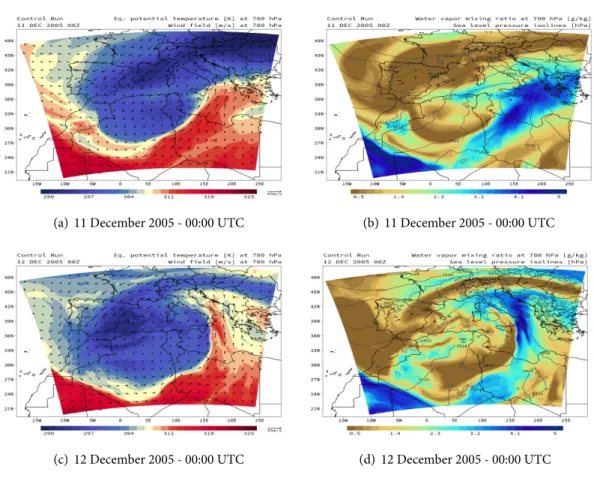
Function (PDF) [18]. . . 25 2.7 Example of spaghetti plot relative to 500 hPa geopotential heights of GFS [7]. 26 2.8 Ensemble tropical cyclone storm track [49]. . . 26 3.1 WRF Modeling System Flow Chart, from the WRF User’s Guide. . . 28 4.1 Medicane Zeo satellite images taken from the MODIS AQUA satellite . . . . 35 4.2 Simulated trajectory of Medicane Zeo - points every 3 hours . . . 36 4.3 Control run temperature field at 500 hPa and sea level pressure surfaces . . 37 4.4 Control runθ_efield at 700 hPa and water vapor mixing ratio at 700 hPa . . . 37 4.5 Moist air back-trajectory analysis at 950 hPa . . . 39 4.6 Moist air back-trajectory analysis at 850 hPa . . . 40 4.7 Moist air back-trajectory analysis at 700 hPa . . . 41 4.8 Isobaric and geopotential height differences between the control run and

the No Fluxes test . . . 43 4.9 Integrated water vapor and water vapor mixing ratio at 1000 hPa in the

control run and No Fluxes test . . . 44 4.10 Sea level pressure isolines in the control run and No Fluxes test . . . 45 4.11 Sea level pressure minimum values (every 3 hours) in the control run and in

No Fluxes test . . . 45 4.12 Dry air back-trajectory analysis at 500 hPa . . . 47 4.13 Dry air back-trajectory analysis at 700 hPa . . . 48 4.14 Dry air at 850 hPa. Comparison with simulation and aerosol reanalysis. . . 49 4.15 Relative humidity field at 300 hPa andθ cross section at ° N for 00Z11-RH50

test. . . 50

4.16 Integrated water vapor with sea level pressure isolines in the control runs

and RH50 tests . . . 52

4.17 Sea level pressure surfaces in the RH50 tests. Surfaces are plotted every 2

LIST OF FIGURES ix

4.18 Sea level pressure minimum values (every 3 hours) in the control runs and

in RH50 tests . . . 54

4.19 Wind speed maximum values (every 3 hours) at 10 m in the control runs and in RH50 tests . . . 54

4.20 θ_efields at 700 hPa of control runs and RH50 tests . . . 55

4.21 θ_ecross sections of control runs and RH50 tests . . . 56

5.1 Medicane Cornelia images in the infrared bandwidth, from the METEOSAT-5 satellite . . . 59

5.2 Simulated trajectory of Medicane Cornelia - points every 3 hours . . . 60

5.3 Control run temperature field at 500 hPa and sea level pressure surfaces . . 61

5.4 Control runθ_efield at 700 hPa and water vapor mixing ratio at 700 hPa . . . 61

5.5 Moist air back-trajectory analysis at 950 hPa . . . 62

5.6 Moist air back-trajectory analysis at 700 hPa . . . 63

5.7 Moist air back-trajectory analysis at 950 hPa . . . 64

5.8 Moist air back-trajectory analysis at 700 hPa . . . 66

5.9 Isobaric and geopotential height differences between the control run and the I No Fluxes test . . . 67

5.10 Integrated water vapor and water vapor mixing ratio at 1000 hPa in the control run and I No Fluxes test . . . 68

5.11 Sea level pressure isolines in the control run and I No Fluxes test . . . 69

5.12 Sea level pressure minimum value (every 3 hours) in the control run and in I No Fluxes test. Dotted part refers to simulation without surface heat fluxes. . . 69

5.13 Integrated water vapor and water vapor mixing ratio at 1000 hPa in the control run and II No Fluxes test . . . 71

5.14 Sea level pressure isolines in the control run and II No Fluxes test. . . 73

5.15 Sea level pressure minimum value (every 3 hours) in the control run (solid blue line) and in II No Fluxes test (dotted+solid green line) and latent heat fluxes maximum values in the control run only (long dash line). Dotted green part refers to the sensitivity test when the heat fluxes have been turned off. . . 73

5.16 Dry air back-trajectory analysis at 500 hPa . . . 74

5.17 Total suface heat fluxes with sea level pressure isolines and wind field at 1000 hPa in the control runs and RH50 tests of 4 October and cyclone simulated trajectories. . . 76

5.18 Sea level pressure minimum values (every 3 hours) in the control runs and

in RH50 tests . . . 77

5.19 Sea level pressure minimum values (every 3 hours) in the control runs and

in RH50 tests . . . 77

5.20 Total suface heat fluxes with sea level pressure isolines and wind field at 1000 hPa in the control runs and RH50 tests of 5 October and cyclone simulated

trajectories. . . 78

5.21 θ_efields at 700 hPa and cross sections of control runs and RH50 tests . . . 79 6.1 Hart’s diagrams of the 00Z12-CTL run and 00Z12-RH50 test cyclones. Colors

are referred to the intensity of the sea level pressure. One point every 3 hours.. . 85 6.2 Hart’s diagrams of the 12Z05-CTL run and 12Z05-RH50 test cyclones. Colors

are referred to the intensity of the sea level pressure. One point every 3 hours.. . 86 6.3 Conceptual model of the detrimental role of upper-level dry intrusions in the

List of Tables

1.1 Saffir-Simpson Hurricane Scale . . . 4 2.1 Space and time scales . . . 17

Acronyms

ABL Atmospheric Boundary Layer AOD Aerosol Optical Depth ARW Advanced Research WRF BOLAM Bologna Limited Area Model CCN Cloud Condensation Nuclei

CFL Courant–Friedrichs–Lewy condition CISK Convective Instability of the Second

Kind

CISL Computational and Information

Sys-tems Laboratory

CNR Consiglio Nazionale delle Ricerche CPS Cyclone Phase Space

DWD Deutscher Wetterdienst Wetter und

Klima aus einer Hand

EC Extratropical Cyclone

ECMWF European Centre for Medium-Range

Weather Forecasts

EOS Electro-Optical System EPS Ensemble Prediction System

ERA5 ECMWF Reanalysis 5th_Generation

FDM Finite Difference Method FT Fourier Transform

GCM General Circulation Model

GEOS-5 Goddard Earth Observing System

Data Assimilation System

GFS Global Forecast System

GOCART Goddard Chemistry, Aerosol,

Radi-ation and Transport

GrADS Grid Analysis and Display System GRIB General Regularly-distributed

Informa-tion in Binary form

HDF Hierarchical Data Format

IFS Integrated Forecasting System model IMEX Implicit-Explicit Method

IPCC Intergovernmental Panel on Climate

Change

ISAC Istituto di Scienze dell’Atmosfera e del

Clima

ITCZ Intertropical Convergence Zone IWV Integrated Water Vapor

LAM Limited Area Model LES Large Eddy Simulations LSM Land Surface Model

MEDICANE MEDIterranean hurriCANE MERRAero Modern Era Retrospective

anal-ysis for Research and Applications Aerosol Reanalysis

MM5 Mesoscale Meteorological Model,

Ver-sion 5

MODIS Moderate-resolution Imaging

Spec-troradiometer

MOLOCH Modello Locale in Hybrid

coordi-nates

NASA National Aeronautics and Space

Ad-ministration

NCAR National Center for Atmospheric

Re-search

NCL NCAR Command Language

NERC Natural Environment Research

Coun-cil

NetCDF Network Common Data Form NHC National Hurricane Center

NMM Nonhydrostatic Mesoscale WRF Model NOAA National Oceanic and Atmospheric

Administration

NWP Numerical Weather Prediction

NWSC NCAR-Wyoming Supercomputing

Center

OI Optimal Interpolation method PBL Planetary Boundary Layer PL Polar Low

PV Potential Vorticity RH Relative Humidity

RRTM Rapid Radiative Transfer Model SLP Sea Level Pressure

SSHS Saffir–Simpson Hurricane Scale SST Sea Surface Temperature

STC Subtropical Cyclone TC Tropical Cyclone TD Tropical Depression TLC Tropical-Like Cyclone TT Tropical Transition

VAPOR Visualization and Analysis Platform

for Ocean, Atmosphere, and Solar Re-searchers

WISHE Wind Induced Surface Heat Exchange WMO World Meteorological Organization WPS WRF Pre-processing System

WRF Weather Research and Forecasting

model

WSM3 WRF Single-Moment 3-class scheme WSM5 WRF Single-Moment 5-class scheme YSU Yonsei University scheme

I

General introduction and

overview of analysis tools

As we got farther and farther away, the Earth dimished in size. Finally it shrank to the size of a marble, the most beautiful marble you can imagine ... seeing this has to change a man. - James Irwin, Apollo 15

1

Introduction to Cyclones

Following the World Meteorological Organization (WMO) official terminology [64], a cy-clone is an area of low pressure, with the lowest pressure at the center, commonly referred to as a Low. Cyclones can form all over the word: above the sea, due to the high sea surface tem-perature (e.g., tropical cyclones) or large temtem-perature difference between sea surface and the air above (e.g., polar lows) or also over land, between warm and cold air masses (e.g., extra-tropical cyclones). Cyclones are grouped into several families with respect to the formation mechanisms and physical features. This work focuses on the MEDIterranean hurriCANEs (MEDICANEs) initial and mature phases; this kind of cyclone is relatively rare with hybrid features typical of the two main cyclone families, tropical cyclones and extratropical cyclones. In this chapter we introduce the main families of cyclones and the necessary nomenclature and terminology in order to refer to these atmospheric phenomena.

1.1

Tropical Cyclones

A tropical cyclone is a rotating storm system with a low pressure center. The most re-markable features of TCs are the presence of an ”eye” of mostly calm weather (figure 1.1), the presence of a warm core, weak vertical wind shear and an eyewall with convective cells. These cyclones mainly form over the tropical oceans near the Intertropical Convergence Zone (ITCZ), within ° to ° latitude degrees from the Equator in both hemispheres. The area most favorable to their formation is 10°; occasionally they may form within 5° of latitude N or S. A starting, although not physics, distinction between the tropical cyclones concerns the place of the world where they form: tropical cyclones over the North Atlantic and Northeast Pacific Oceans are called hurricanes, while those over the Northwest Pacific Ocean are called typhoons and simply cyclones for the rest of the world.

The typical atmosphere where the TCs develop is called the barotropic atmosphere: it means that the density of the fluid (the air) is a function of pressure only, so the isobaric surfaces are also surfaces of constant density. Furthermore, the isothermal surfaces coincide with isobaric surfaces. From the thermal wind equation:

∂Vg

∂ ln p = − Rfk × ∇pT (1.1)

Figure 1.1– Hurricane Michael, October 10, 2018. Image take from the NOAA website [50]

Category

Wind speed

m/s km/h Types of damage

1 33-42 119-153 Very dangerous winds will produce some damage 2 43-49 154-177 Extremely dangerous winds will cause extensive damage

3 50-58 178-208 Devastating damage will occur

4 58-70 209-251 Catastrophic damage will occur

5 ≥  ≥  Catastrophic damage will occur

Table 1.1– Saffir-Simpson Hurricane Scale

the geostrophic wind will not vary with depth in a barotropic atmosphere, because the term ∇_pT is zero, due to the absence of a temperature gradient along isobaric surfaces. It is not clear how tropical cyclones form but, according the observations, there are some conditions that are requested to create a favorable environment for the formation of a cyclone: sea surface temperature above .° C in an ocean layer of 50 m of depth; a large vertical lapse rate; a distance generally of about ° from the Equator so that the rotation can be derived from the Coriolis effect; finally, weak vertical shear. If the initial perturbation develops in a favorable environment, it will grow into a Tropical Depression (TD) and it may evolve further into a TC. The intensity and the potential impact on the human environment of the TCs is provided by the Saffir–Simpson Hurricane Scale (SSHS) (table 1.1).

Figure 1.2 shows the structure of a typical TC. The main energy sources of the TC are the sensible and latent heat fluxes from the surface of the tropical oceans and the latent heat released from the condensation of water vapor. In fact, these systems are characterized by a warm core due to the huge quantity of latent heat released by condensation. To explain how the

. | Tropical Cyclones 5

Figure 1.2:Simplified model of the structure of a TC in the Northern Hemisphere. Images taken from the Encyclopedia Britannica [65]

TCs develop and their main maintenance mechanisms, two fundamental approaches have been proposed. The first, by Charney and Eliassen, 1964 [11], is called the Convective Instability of

the Second Kind (CISK) theory; CISK is a positive feedback mechanism that causes the

ampli-fication and the maintenance of the original disturbance. The convergence of winds toward a low pressure minimum at the surface triggers convection, which then causes cumulonimbus formation and the release of latent heat associated with the condensation of boundary-layer water vapor. Since the latent heat warms the air column, the warming causes an increased vertical destabilization of the environment and, together with the expansion of air, there is a reduction of the surface pressure. When the surface pressure decreases, a larger surface pres-sure gradient is formed and additional air converges towards the center of the storm. This mechanism can sustain itself until other factors, such as the advection of cold and dry air, or high wind shear act to weaken it. However, this theory does not take into account the heat fluxes from the surface. According to the CISK theory, TCs may form wherever the energy of the atmosphere can supply the ”fuel” for the cyclone formation. A second theory that takes into account the heat fluxes from the surface and completes the CISK theory was formulated by Emanuel and Rotunno in two papers [21, 59]. According to this air-sea interaction theory, aka the Wind Induced Surface Heat Exchange (WISHE) mechanism, a TC can be viewed as a heat engine that converts the heat stored in the water evaporated from the sea into mechanical energy. This kind of phenomenon is self-sustaining as long as it has warm water from which to gain the energy: the role of the TC vertical motion is to redistribute the heat acquired from sea surface to keep the environment locally neutral; the consequent decrease of the sea level pressure increases the intensity of the winds, promoting increased evaporation and condensa-tion.

way in the Northern Hemisphere and vice-versa in the Southern Hemisphere. In a mature TC, air sinks rather than rises at the center, forming an ”eye” of clear air without wind; this feature is due to the descending air from the top of the troposphere, where the air goes down to the center becoming warmer and dissipating the clouds. The diameter of the eye is about - km while the typical size of the whole cloud structure of a TC is within mesoscale values, from km to  km for a very large cyclone; the vertical extent reaches the tropopause, which is  − km at tropical latitudes [6].

1.2

Extratropical Cyclones

The second main family of cyclones is formed by extratropical cyclones. As their name suggests, this class of cyclones forms outside the tropics, between ° and ° latitude in both hemispheres. Figure 1.3 shows a nor’easter, which is an extratropical cyclone in the western North Atlantic Ocean where the winds typically blow from the northeast along the US east coast. According to the glossary of the Intergovernmental Panel on Climate Change (IPCC) 5th Assessment Report, an EC is a synoptic (of order 1000 km) storm in the middle or high lat-itudes having a low central pressure and fronts with strong horizontal gradients in temperature and humidity. ECs can arise from cyclogenesis or by extratropical transition of TCs. Especially in winter, when the anticyclonic dominant patterns in summer (e.g., Azores High) lose inten-sity and the jet stream moves southward, cold and dry air masses can meet with warm and wet air masses, especially over the oceans. In these cases, a temperature and dewpoint gradient, called frontal zone, exists. Since the air density depends on both temperature and pressure, isobaric and isothermal surfaces are no longer parallel and the atmosphere is called baroclinic. The related baroclinic instability is of fundamental importance to understand midlatitude

Figure 1.3:Powerful Nor’easter off the United States Atlantic coast on March 26th 2014. Image taken from Suomi NPP satellite [25]

. | Extratropical Cyclones 7

Figure 1.4: Horizontal and vertical simplified cross section of an EC

cyclogenesis. A typical environment favorable to EC development consists of an upper-level distur-bance which is due to a downward undulation of the tropopause and a frontal zone in the lower-levels. In contrast to a barotropic atmosphere, in a baroclinic environment the geostrophic wind generally has ver-tical shear, related to a meridional temperature gra-dient by the thermal wind equation (equation 1.1). The presence of a jet stream in the upper level im-plies vorticity at its sides. The upper-level distur-bance has an effect on the lower level flow such that a low (high) pressure is generated below a region of upper-level divergence (convergence). The circula-tion induces two regions of large thermal gradient

(cold and warm fronts), rotating around the cyclone center. In the mature stage, the cold front reaches the warm front. The reason why the cold front is faster than the warm front is not trivial, because several dynamical and thermodynamic effects compete. However, in a first ap-proximation, the heavier, denser, cold air can push the warmer, lighter air ahead of the cold front out of its way much more easily than the warm air (which is lighter and tends to move above the cold air) can push the cold air ahead of the warm front. The cold front wedges under the warm front: thus, warm and wet air is violently displaced (figure 1.5). The warm front in the upper levels wraps around the pressure minimum, which occurs in the later stages of the cyclone lifetime, while cold air blows into the minimum from lower levels. The station-ary presence of both cold and warm fronts in the vicinity of the minimum takes the name of occluded front. The most intense precipitation phenomena are located just ahead of the cold front, while stratiform and lighter precipitation are found in the warm section.

One of the main differences between TCs and ECs is that the latter have an asymmetric and tilted cold core. In figure 1.4 are represented, in a very simplified way, a horizontal (upper figure) and a vertical (lower figure) section of an EC. In the lower figure, the white lines are geopotential heights at fixed pressure. To explain why ECs have a cold-core, we can use the hypsometric equation 1.2:

Φ(z) − Φ(z) = g(Z− Z) = R

∫

p

Td(ln p) (1.2)

where Φ(z) is the geopotential, Z ≡ Φ

g is the geopotential height (in the troposphere Z is

numerically almost identical to the geometric heightz). Equation 1.2 states that the variation in geopotential with respect to pressure depends only on temperature. Hence, the thickness of an atmospheric layer between two isobaric surfaces is proportional to the mean temperature of

Figure 1.5– Simplified model of the structure of an EC, from Cloud Dynamics book [58]

the layer. Thus, referring to the lower panel in figure 1.4, closely spaced geopotential isolines mean colder air.

The development and dynamics of ECs are quite complicated with respect to TCs and some models (e.g. the Norwegian model [1] - figure 1.6 or the Shapiro-Keyser model [60]) have been proposed to explain the extratropical cyclone life cycle. An interesting feature of ECs is the formation, in its later stages, of a region of warm air near the pressure minimum, called the warm seclusion. This area may have an eye-like feature, significant pressure falls and strong convection. These features look like the main characteristics of TCs. In the Mediterranean Tropical-Like Cyclones section, we will see that the warm seclusion may promote tropical-like features, such as a warm core and the presence of an ”eye”.

Figure 1.6– Schematic representation of the Norwegian model, from Bjerknes and Solberg, 1922 [2]

. | Polar Lows 9

1.3

Polar Lows

Figure 1.7:A PL off the NW coast of Norway on April 6th 2007. Image taken from NERC receiving station [48]

Businger and Reed, 1989 [4] define a Po-lar Low (PL) as any type of small synoptic-or subsynoptic-scale cyclone that fsynoptic-orms in a cold air mass poleward of major jet streams or frontal zones and whose main cloud mass is largely of convective origin. In the early stage of formation, PLs can form a comma-shaped structure that is very similar to that of ECs. In their mature stage, PLs as-sume a Tropical-Like Cyclone (TLC) struc-ture, with clouds surrounding a cloud-free ”eye” and a warm core (Emanuel and Ro-tunno, 1988 [59]), which has given rise to the use of the term Arctic hurricane to describe some of the most active lows, as in figure 1.7. Due to the large values of the Coriolis parameter in the polar regions, PLs have smaller di-ameters than those of TCs. Reale and Atlas, 2001 [56] noted that in the Mediterranean TLCs latent-heat fluxes are much stronger than sensible-heat fluxes, while in the PLs latent and sen-sible fluxes are normally comparable. The underlying causes of polar lows are a combination of baroclinic and barotropic instabilities, which means that its energy derives from both the horizontal temperature gradient and the relatively warm ocean waters with respect to the cold air above; similarities with both TCs and ECs put PLs into a hybrid cyclones category and a rigorous formation and classification theory is still the subject of research.

1.4

Subtropical Cyclones

Following the definition of the National Hurricane Center (NHC), a STC is a non-frontal low pressure system that has characteristics of both tropical and extratropical cyclones. These hy-brid cyclones generally form from an EC that moves toward subtropical latitudes above warm waters or when a cold upper level low is moving in over the subtropics, below ° latitude in both hemispheres; because of the presence of cold air in the initial disturbance, STCs need lower sea temperatures than do TCs (around °C) to trigger deep convection. While the ori-gin of a STC is mainly due to baroclinic instability and is characterized with an initial cold core center, in its mature stage, if the subtropical storm remains over warm waters for several days, it may sustain itself mainly through barotropic processes and acquire a warm core, as in a TC.

Figure 1.8:STC Katie at east-southeast of Easter Island at 21:25 UTC, May 2nd 2015.

Image taken from Suomi NPP satellite [24]

These storms have generally larger horizon-tal cloud extents with respect to TCs, weaker convection and a less symmetric wind field. Unlike traditional TCs, where the strongest winds are concentrated around the center (where the thunderstorm activity is more in-tense as well), in STCs these two features are displaced far from the center of circulation. If the maximum sustained winds are greater than or equal to  m/s they are called sub-tropical storms. The most famous STCs are: the Australian east coast lows, which affect the south coast of the island, the Kona storms which are a type of seasonal cyclone near the Hawaii, and the MEDICANEs.

1.5

Mediterranean Tropical-Like Cyclones

These types of cyclone, often unofficially referred to MEDICANEs or Mediterranean TLCs, are meteorological phenomena observed over the Mediterranean Sea, that can occasionally reach category 1 on the Saffir-Simpson scale. There is no official meteorological definition of medicane, but the term is often used to describe a deep area of low pressure characterized by a warm core, deep convection around the pressure minimum, strong winds and thunderstorm activity that sometimes has the appearance of a hurricane. Figure 1.9 shows Medicane Numa after peak intensity, where the presence of an ”eye”, typical feature of a TC, is clearly visible over the Ionian Sea. MEDICANEs form a small class of subtropical cyclones, extract avail-able potential energy through baroclinic processes in the early stages, as in an EC, but they receive some or most of their energy from condensational heating, as do TCs in their mature stage. Therefore, MEDICANEs form by Tropical Transition (TT), which is the dynamic and thermodynamic transformation of an EC into a TC.

The first studies of this type of cyclone are from Ernst and Matson, 1983 [22] and Ras-mussen and Zick, 1987 [54], where the first satellite images showed the similarity with Atlantic hurricanes. Triggering mechanisms for the MEDICANEs are not yet well understood, but some aspects have been studied. MEDICANEs develop in the western and central Mediter-ranean basin, a geographic area surrounded by several mountain ranges (e.g., Alps, Pyre-nees, Atlas Mountains); convection may be promoted by orographic lift (Buzzi and Tibaldi, 1978 [5]) or lee cyclogenesis (Moscatello at al., 2008 [44]). The Mediterranean basin is also a highly baroclinic region: ECs forming due to wind vertical shear over the sea may,

occasion-. | Mediterranean Tropical-Like Cyclones 11 ally, create a favorable environment for mesoscale vortexes similar to hurricanes (Reale and Atlas, 2001 [56]); in that circumstance, if surface heat fluxes from the Mediterranean Sea are intense enough to provide moist air, convection will sustain itself, so that the environment be-comes more barotropic and tropical features may eventually appear, due to diabatic heating of the midtroposphere.

Figure 1.9:Medicane Numa over the Ionian Sea at 09:25 UTC, November 18th 2017. Image taken from MODIS website [45]

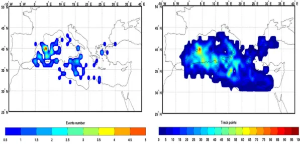
One of the most relevant differences in the MEDICANEs formation process with respect to that of TCs is the role of precursors in the higher troposphere. MEDICANEs generally form in correspondence to a deep upper-level cold cut-off low that destabilize the atmospheric column (Homar et al., 2003 [31], Moscatello et al., 2008 [44], Emanuel, 2005 [20]). This circumstance preferentially occurs during fall or early winter (figure 1.10), i.e. when the dominant summer anticyclonic pattern loses intensity and troughs from the polar vortex can reach southern re-gions, finding relatively warm and moist air below. So the main source of potential energy to trigger convection is the thermodynamic disequilibrium between the atmosphere and the underlying sea. A majority of MEDICANEs forms generally over two regions: the western Mediterranean north of the Balearic Islands and west of Sardinia and Corsica, and the Ionian Sea between Sicily and Greece down to Libya (figure 1.11). The frequency of MEDICANEs occurrence is extremely low, 1.57 ± 1.30 events per season, as such they can considered as rare events (Cavicchia at al., 2012 [8], Nastos et al., 2018 [47]).

Beside this remarkable difference with respect to TCs, surface-heat fluxes play the crucial role to allow the formation and especially the intensification of MEDICANEs; as in the case of TCs, the mechanism of air–sea interaction, expressed in the WISHE theory, is crucial for TLCs intensification. Part of the present work will show that if the sensible and latent heat fluxes from

Figure 1.10: Number of medicanes per month (total number in the period 1948–2011). Image taken from Cavicchia at al. [8]

(a) Genesis density (first location in the track) per ° × ° box.

(b) Track density per ° × ° box.

Figure 1.11: Locations of all the medicanes detected for the period 1948–2011. Images taken from Cavicchia at al. [8]

the sea are turned off during the numerical simulation, the cyclone will not form at all. This fact is confirmed by several studies (Pytharoulis et al., 2000 [52], Miglietta et al., 2011 [40], Tous and Romero, 2012 [63] and others). A couple of recent papers (Fita and Flounas, 2018 [26]; Mazza et al., 2017 [38]) have raised some doubts concerning the mechanism of two Mediter-ranean TLCs, supporting the idea that the warm-air seclusion in the extratropical cyclone’s inner core may be sufficient to explain the presence of a deep warm, core structure. Miglietta and Rotunno, 2019 [42] performed sensitivity experiments for the two TLCs without latent-heat release and/or sea-surface fluxes, showing that the air–sea interaction and the latent latent- heat-ing due to convection are necessary in order to explain the intensification of both cyclones,

. | Mediterranean Tropical-Like Cyclones 13 and suggesting a key role for the WISHE mechanism in the cyclone development. However, the importance of air-sea interaction appears to be case dependent.

Another noteworthy similarity between MEDICANEs and TCs formation concerns the role of the Sea Surface Temperature (SST). Several papers focused on the SST: sensitivity tests performed by Fita et al., 2007 [27] and Miglietta at al., 2011 [40], Pytharoulis et al., 2018 [53] show that the cyclone loses intensity and typical tropical features disappear if the SST is pro-gressively reduced with respect to the control run.

Concerning the classification algorithm, a unique and objective method to identify and classify a cyclone as MEDICANE does not exist. To understand the various types of synoptic-scale cyclones in a unified framework, Hart, 2003 [29] proposed a cyclone classification algo-rithm called Cyclone Phase Space (CPS), or Hart’s diagram. The CPS assesses cyclone types objectively based on their geometric and thermal symmetry structure, once identified in atmo-spheric gridded datasets, such as reanalysis and model simulations: a TC is a deep warm-core, symmetric cyclone, whereas an EC is a deep cold-core, asymmetric cyclone. An STC is in-termediate between a TC and an EC, since it has a shallow warm-core (a warm core in the lower troposphere, but a cold core in the upper troposphere) structure (Evans and Guishard, 2009 [23]). The CPS describes the cyclone phase using three parameters:

• the storm-motion-relative 900-600 hPa thickness asymmetry across the cyclone within 500-km radius:

B = h (Z− Z∣R− Z− Z∣L) (1.3)

whereZ is isobaric height, R indicates right of current storm motion, L indicates left of storm motion, the overbar indicates the areal mean over a semicircle of radius 500 km, andh takes a value of + for the Northern and − for the Southern Hemisphere;

• the cyclone thermal wind parameter in the lower troposphere, defined as the vertical derivative of horizontal height gradient between 900 and 600 hPa:

∂ (∆Z) ∂ ln p ∣   = − ∣VL T∣ (1.4)

where ∆Z = Z_MAX− Z_MINis the cyclone height perturbation and it is evaluated within a radius of 500 km, consistent with the radius used for the calculation ofB; L means ”lower”;

• the cyclone thermal wind parameter in the upper troposphere, defined as the vertical derivative of horizontal height gradient between 600 and 300 hPa:

∂ (∆Z) ∂ ln p ∣   = − ∣VU T ∣ (1.5)

Hart proposes also thresholds on the values of these parameters to distinguish between warm- and cold-core structures. He states that a cyclone has a warm core if:

• B <  m • − ∣V_TL∣ >  • − ∣V_TU∣ > 

This CPS provides an objective classification of the cyclone phase, “unifying the basic struc-tural description of tropical, extratropical, and hybrid cyclones into a continuum” (Hart, 2003 [29]). Transitions between cold- and warm- core structure can be objectively identified, including extratropical transition, tropical transition, warm seclusions and the development of hybrid cyclones, all of which are summarized in figure 1.12.

This classification algorithm was used in the last few years by Gaertner et al., 2008 [28] in a future scenario of climate change over the Mediterranean region, by Chaboureau et al., 2012 [10], readapting the radius of the circles for the calculation of the diagram for Mediter-ranean storms to 200 km, and by Miglietta et al., 2011 [40] and 2013 [41], readapting the radius of the circle respectively to 100 km and to the extent of the warm core anomaly at 600 hPa for the MEDICANEs. Through this approach Miglietta et al., 2013 [41] drafted a list of tropical-like cyclones events in the Mediterranean region. Picornell et al., 2014 [51] used shallower depths for MEDICANEs, taking into account that their vertical extension, which is more lim-ited compared to TCs.

(a) -VL

T vsB (b) -VTLvs -VTU

2

Models

2.1

Overview

Generally speaking, a model is a mathematical, physical and chemical representation that can diagnose the past or present, or attempts to predict the future, state of a real system. A weather-prediction model solves the primitive equations based on current physical and chemi-cal knowledge. The first attempt to solve those equations was due to L. F. Richardson, however his 6h surface pressure tendency prediction was very unrealistic. The solutions of Richard-son’s equations contain not only slow-moving waves but also high-velocity phenomena, such as sound and gravity waves; these kinds of waves tend to amplify and produce ”noise” obscur-ing more relevant meteorological phenomena. This problem can be solved with an appropriate approximation of the primitive equations based on the time and length scales of the relevant phenomena, as we will see later. Another problem was the lack of knowledge of initial condi-tions: according to V. F. K. Bjerknes [3], weather prediction is mainly an initial-value problem; thus, it is necessary to know with great precision both the laws governing atmospheric motions and the physical and thermodynamic state of the atmosphere at a certain initial time. Fortu-nately, improvements in physical knowledge, the systematic use of atmospheric soundings for the analysis of the atmosphere and the increase in computer processing power have allowed the improvement of weather prediction, which is now approaching the theoretical limit of two weeks foreseen by E. N. Lorenz [36]. Nowadays, meteorological models can be grouped in two main classes:

• General Circulation Models (GCMs), like the USA GFS, European Integrated Forecasting

System model (IFS) or the GLOBO model developed by the Italian Consiglio Naziona-le delNaziona-le Ricerche (CNR). This kind of model covers the whoNaziona-le atmosphere, describing synoptic systems with an approximate horizontal resolution of tens of km. They are run operationally every day to provide forecasts of meteorological fields at medium range (< three weeks) and their output can be used as initial and boundary conditions for the following class of models;

• Limited Area Models (LAMs), like WRF, the Bologna Limited Area Model (BOLAM)

(which is hydrostatic) or the Modello Locale in Hybrid coordinates (MOLOCH) (which 15

is nonhydrostatic; the last two were both developed by CNR), cover a smaller part of the atmosphere (e.g., part of a continent or one region). These models are the best choices to make an accurate prediction in a local area, since, compared to GCM, they have a finer grid spacing that can reach up to few km or even hundreds of meters. Generally, LAMs are run only for short-range, forecast for example, BOLAM model provides operational forecast within a range of  days with . km grid spacing. LAMs are forced by GCM, so their outputs are not independent of the large-scale fields used to force these models. The extension and the resolution of the LAM domain are a compromise between the need to properly represent small-scale features and to use a finite amount of computational power. These types of models are used to predict mesoscale orα–microscale weather systems.

2.1.1 Prognostic models

All prognostic models (that is, where time is an explicit variable) predict future state of systems, knowing initial conditions of the atmosphere. First of all, they cover the atmosphere with a 3D grid covering the whole globe (GCM) or a limited area (LAM) with a suitable hor-izontal and vertical spacing. The following equations, in the form taken from the book An Introduction to Dynamic Meteorology [30], have to be solved:

D U D t = −Ω × U −  ρ∇ p + g + Fr Momentum Equations (2.1)  ρ D ρ D t + ∇ ⋅ U =  Continuity Equation (2.2)

cνD T_{D t} + L D q_{D t} + p D α_{D t} = ˙Q Energy Conservation Equation (2.3)

D q

D t = ˙Pq Humidity Conservation Equation (2.4)

pα = RdTν State equation (2.5)

where Ω is the angular velocity of Earth,ρ is the density, p is the environment pressure, g is the gravity term, F_r are the frictional forces,c_ν is the specific heat of dry air at constant volume, T is the environment temperature, L is the latent heat, q is the water vapor mixing ratio, α is the specific volume, ˙Q is the diabatic heating rate, ˙P_qis the sum of all the source and sink rate terms ofq in the atmospheric column, R_dis the gas constant for dry air andT_vthe virtual tem-perature. Some of previous equations can be simplified according to the typical space and time

. | Parameterizations 17 scale one wants to investigate, indicated in Table 2.1, where the last row refers for Large Eddy Simulations (LES). Scale analysis leads to hydrostatic (equation 2.6) and geostrophic approx-imation (equations 2.7 and 2.8) in synoptic scale. The hydrostatic approxapprox-imation is generally used in GCM and LAM with grid spacing greater than - km.

Models Horizontal Scale Vertical Scale Range Time

Climate models km m years

GCM km m days

LAM km m days

Cloud model m m day

LES m m hours

Table 2.1– Space and time scales

∂ p

∂ z = −ρg Hydrostatic approximation (2.6)

vg = _{f ρ} ∂ p_{∂ x} Zonal component of geostrophic wind (2.7)

ug= −_{f ρ} ∂ p_{∂ y} Meridional component of geostrophic wind (2.8)

2.2

Parameterizations

Since horizontal resolution is limited, some phenomena cannot be resolved by models be-cause their typical space scale is smaller than grid spacing or their behaviors are too complex to be physically represented by a simplified process; this kind of phenomenon is said to be subgrid scale and needs to be statistically analyzed. The procedure of expressing the effects of subgrid processes is called parameterization.

2.2.1 Radiation

As it is well known, the energy of the Sun is the main source for the atmospheric motions. An indication of this at the largest scales is the differential heating from the poles to equator that drives the mean global circulation. The local energy budget depends on many factors: the solar zenith angle, the albedo of the surface, the temperature of the emitting body and its emissivity, the local cloud type fraction, etc. An accurate representation of radiative processes and their time and space variations are essential for weather and climate research.

Figure 2.1– Overview of sub-grid proceses, from ECMWF website [17].

Radiation is divided into short and long-wave components: short-wave directly comes from the Sun and it can be absorbed by surfaces or atmospheric gases or scattered back, while long-wave radiation is emitted by surfaces and the Earth’s atmosphere. If the incoming radi-ation is absorbed or reflected from an object, it will depend on the radiative properties of the object itself (type of soil, type and concentration of a certain gas, etc.) and the frequency of the radiation. In the same way, the amount of emitted long-wave radiation will depend on the radiative properties of the object. Computationally, it is too expensive for a meteorolog-ical model to deal with all the lines of the spectrum of radiation; thus, the spectrum is split into different frequency bands, where each of these has different capacity of interaction with the atmospheric gasses and particles (like, water vapor, ozone and carbon dioxide). Types of radiative transfer model that have been used in this work are: the Rapid Radiative Transfer Model (RRTM) scheme (Mlawer et al., 1997) [43] for long-wave radiation and the Dudhia scheme (Dudhia, 1989) [15] for short-wave radiation.

2.2.2 Convection

In the atmosphere, the phenomenon of convection can occur when an air mass is heated by an energy source (the Sun) and its density becomes smaller than the surrounding air, so that the air parcel may ascent: in this case we refer to free convection. Instead, when an air mass is forced up either by a colder air mass moving in the low-levels (e.g., mid-latitude fronts) or by orographic lift, we refer to forced convection. In any case, convection probably represents the most important physical process to parameterize in order to forecast weather. Especially free convection occurs on small horizontal scales, of the order of km or less. Convection can also be distinguished in shallow convection or deep convection: the first, where updraft velocities are of the order of fewm/s, generally forms low stratified clouds, with an horizontal extent

. | Parameterizations 19

Figure 2.2– Earth’s energy budget, from NASA website [46].

much greater than the vertical; the second occurs when surface heating is very strong or in presence of deep atmospheric instability (e.g., cumulonimbus formation); in this case, impres-sive vertical cloud structures are formed, even passing above the tropopause. Deep convection is associated with the most intense and dangerous weather phenomena; to predict these events with a suitable advance time for civil protection purposes, the models do not need only an high horizontal resolution but a high vertical resolution as well. The Kain-Fritsch (Kain, 2004) [35] scheme has been used for cumulus parameterization; this scheme reproduces local shallow and deep convection, furthermore it allows the resolution of the vertical flux due to updraft and downdraft motions that are not solved on the grid.

2.2.3 Land-Surface models

Land Surface Models (LSMs) use quantitative methods to simulate the biogeochemical, hy-drological and energy cycles at the Earth surface–atmosphere interface. A LSM must provide four quantities to the atmospheric model: surface sensible-heat fluxQ_H, surface latent-heat fluxQ_E, upward long-wave radiationQ_L(or skin temperature and surface emissivity) and up-ward (that is, reflected) short-wave radiation Q_S (or surface albedo). These fluxes provide lower boundary conditions for vertical motions. To parameterize land effects, a 5-layer ther-mal diffusion scheme (Dudhia, 1996) [16] has been used here.

2.2.4 Clouds

A cloud is defined as an aggregate of very small water droplets, ice crystals, or a mixture of both, with its base above the Earth surface. With the exception of certain types that have no di-rect effects on weather, clouds are confined to the troposphere. They are formed mainly as the result of vertical motion because of air heating, in forced ascent over high elevations, or in the

large-scale vertical motion associated with depressions and fronts. At temperature below  °C, cloud particles frequently consist entirely of supercooled water droplets down to about − °C in the case of layer clouds and to about − °C in the case of convective clouds. At temperature between supercooled limits and about −. °C, clouds are ”mixed” in water droplets and ice crystals. Below −. °C, clouds are mainly compound of ice crystals. Formation and dynamics of the clouds are strictly connected with chemical processes: except from really low tempera-tures (that can be reached in the upper troposphere), formation of embryonal cloud droplets occurs through specific atmospheric aerosols called Cloud Condensation Nuclei (CCN). The latter are minute solid particles suspended in the atmosphere, on which water vapor condenses at typical supersaturated relative humidity values detected inside clouds. This kind of forma-tion is called heterogeneous nucleaforma-tion (as opposed to homogeneous nucleaforma-tion, which occurs below −. °C); in this case, water vapor does not need a solid surface to induce condensation. After formation, droplets can grow in many different ways, which in fact are not all known or completely understood, to become drops, raindrops, graupels or hail. Cloud parameterization has to consider all kinds of processes, many of which are governed by stochastic equations, that take place at microscopic scales. In order to parameterize microphysics processes, in this work we have been used the WRF Single-Moment 5-class scheme (WSM5) (Hong, Dudhia and Chen, 2004) [32], a slightly more sophisticated version of the WRF Single-Moment 3-class scheme (WSM3), that allows for mixed-phase processes and super-cooled water.

Figure 2.3: Overview of microphysic processes that take place inside clouds, from Cloud Dynamics book [58].

. | Numerical Methods 21

2.2.5 Turbulence

The Atmospheric Boundary Layer (ABL), or Planetary Boundary Layer (PBL), is that por-tion of the atmosphere affected by the presence and properties of the underlying surface and biosphere. The depthh of the PBL varies typically from  m to _{m, in relation to the type}

of surface, hour of the day and season. Compared to the longer time scale involved in phe-nomena that affect the whole atmospheric depth from the surface the to tropopause, this tiny layer of atmosphere has a time scale of variations of one hour. PBL phenomena are essentially turbulent, and hard to mathematically analyze, due to the stochastic behavior of mixing pro-cesses. There is not a complete and unified theory of turbulence but different approaches to study it, as Reynolds or Kolmogorov theories with countless empirical formulas. The Yonsei University scheme (YSU) (Hong, Noh and Dudhia, 2006) [33], a non-local-K scheme with explicit entrainment layer and parabolic K profile in unstable mixed layer, has been used to parameterize the PBL, while the revised Mesoscale Meteorological Model, Version 5 (MM5) Monin-Obukhov scheme (Jiménez et al., 2012) [34] has been chosen to parameterize the sur-face layer.

Figure 2.4– Overview of turbulence processes that take place in the atmosphere [62]

2.3

Numerical Methods

The goal of numerical forecast is to determine the future state of the atmosphere, knowing its initial state, with appropriate numerical approximations. In addition to a good knowledge of the current state of the atmosphere, we need a closed system of equations, numerical methods to integrate them and, naturally, powerful supercomputers. A problem with the complete set

of equations is that they contain waves-like solutions (i.e., sound and gravity waves) that are not of meteorological interest and produce ”noise” that obscures the relevant meteorological fields. As anticipated earlier, appropriate approximations can be used as a filter to obtain a set of equations without the presence of sound and/or gravity waves.

Even the equation of barotropic vorticity, the simplest prognostic equation, is nonlinear and has a complicated solution; other equations contain terms depending on Uand cannot be solved analytically. A way used in almost all Numerical Weather Prediction (NWP) models to solve these difficulties, is to use the so called Finite Difference Methods (FDMs). FDMs are discretization methods for solving differential equations by approximating them with differ-ence equations, in which derivatives are approximated with finite differdiffer-ence of desired order of accuracy. If Ψ(x) is the solution of the differential equation in a certain interval, we can divided the interval inJ sub-intervals of length dx, so called grid spacing; now we can approx-imate Ψ(x) with J +  values:

Ψj(x) = Ψ(j dx)

Ifdx is much smaller than the length scale in which Ψ(x) varies, Ψ_j(x) will be a good ap-proximation for Ψ(x). A greater accuracy can be achieved with a smaller dx, but this implies an increase in the number of points, or an increase in the degree of the polynomial used for the approximation (which may lead to very complicated formulas). Approximate solutions must be limited on the numerical domain, otherwise numerical methods become unstable. The Courant–Friedrichs–Lewy condition (CFL) sets strong limitations on the Courant num-berσ = c_{d x}d t. In the case of explicit methods,σ must be less or equal , thus, grid spacing and integration time have to be chosen carefully. Explicit methods solve the equation in a foreward way, knowing the current approximate value of the solution and moving it on in time and space. Implicit methods, instead, find a solution by solving the equation involving both the current and future state of the system. Numerical analysis shows that implicit methods are absolutely stable, therefore the solution does not grow with time. Incidentally, implicit methods are more complicated to deal with because they have to solve the equation in all grid point directions simultaneously and leads to the calculation of huge matrices, which is historically one of the most time-consuming computational problems. Moreover, implicit methods cannot be used if there are nonlinear terms: a solution is to use Implicit-Explicit Methods (IMEXs), where nonlinear terms are treated in an explicit way.

Another method used in some meteorological models (like the glsecmwf IFS) is the spec-tral method; the variations of space variables are expressed as a function of finite series of orthogonal functions. In case of sphere-like domains as the Earth, spherical harmonics are used as orthogonal functions. At low resolution (that is, for GCMs), spectral methods are more accurate than FDM (e.g., a single Fourier component can realistic represent one Rossby wave, while many points are required for FDM). On the other hand, spectral methods have

. | Data Assimilation 23 serious computational problems when there are many components of spherical harmonics be-cause of nonlinear nature of the advection terms. This problem can be solved using the Fourier Transform (FT) that allows us to switch from spherical harmonics’s wave numbers to latitude-longitude grids at each time step; the advection term can be treated on this new grid, avoiding to calculate spectral function products.

Current NWP models are based on approximate primitive equations. Vertical coordinates are generally terrain-following. Anyway, surface is not flat and pressure will change: to avoid complication due to vertical-dependent boundary conditions, the so called σ coordinate is used:

σ = _pp − pT

S− pT (2.9)

where p is pressure, p_T is the pressure at the top of the model and p_S is the mean sea level pressure;σ =  at the ground and  at the top. Thus, σ condition is  everywhere on the lower surface, even if there is an obstacle. Primitive equations inσ coordinates will be:

D U D t + f k × U = −∇Φ + σ∇ ln ps ∂ Φ ∂ σ Momentum Equation (2.10) ∂ps ∂ t + ∇ ⋅ (psU) +ps ∂ ˙σ ∂ σ =  Continuity Equation (2.11) ∂ Φ ∂ σ = − Rθσ ( pp )k Hydrostatic Equation (2.12) ∂ θ ∂ t + U ⋅ ∇θ + ˙σ ∂ θ∂ σ = Jcp θ T Thermodynamic Equation (2.13) D qv D t = Pv Moisture-Continuity Equation (2.14)

where U = (u, v), Φ is the geopotential, θ is the potential temperature, pis  hPa,qvis the

mixing ratio andP_vthe source term. Primitive equations are solved on a particular type of grid on which all of the variables are not predicted at all of the points but rather are interspersed at alternate points. This kind of grid is called ”staggered”. Vertical staggered grid is telescopic, that is, there is higher level density near the ground and lesser near the top of the model, due to the high resolution needed in the lower atmosphere.

2.4

Data Assimilation

Data assimilation is a mathematical discipline that seeks to optimally combine theory with observations. Objective of atmospheric data assimilation is to produce a regular and physically

consistent representation of the state of the atmosphere from a heterogeneous array of in situ and remote instruments, which sample the atmosphere imperfectly and irregularly in space and time. Data assimilation extracts the signal from noisy observations, interpolates in space and time and reconstructs state variables that are not sampled by the observation network.

One of the major problems of NWP is the knowledge of initial conditions. Observations cannot be used directly but they need to be modified to be dynamically valid. In NWP, data assimilation combines observation of meteorological variables, such as temperature and atmo-spheric pressure, with prior forecast in order to initialize numerical forecast models.

Figure 2.5– Assimilation Scheme [9]

Optimal Interpolation methods (OIs) calculate optimal values of weights to minimize the error of the variance. The generic formula is:

xa= xb+ W (y − H (xb)) (2.15)

where x_a is the result of analysis, x_b is the forecast (or background) vector, y is the obser-vation vector, H is a non-linear operator that converts the background in obserobser-vations (e.g., radiative transfer equations) and W is the matrix of weights, whose elements are functions of background and observation errors. OIs directly solve the problem.

An alternative approach is to iteratively minimize a cost functionJ(x) that solves the same problem. These are called variational methods, such as 3D or 4D variational data assimilation: 3D-VAR is formally equivalent to OI methods, while 4D-VAR method uses the model to create a sequence of states that fit optimally with background and the observations on a time frame. In 4D-VAR, observations are included from following and previous time steps into the analysis. The main advantages of 4D-VAR are the consistency with the governing equations and the implicit links between variables; on the other hand, these methods are computationally very expensive and the model result may be too constrained.

. | Ensemble Forecasting 25

2.5

Ensemble Forecasting

Ensemble Forecasting is a method used to evaluate and quantify the two usual sources of uncertainty in forecast models, that is, the errors introduced by the use of imperfect initial condition amplified by the chaotic nature of the atmosphere equations, and errors introduced because of imperfections in the model formulation, such as approximate methods and different types of parameterizations. In practice, several forecasts of similar models are run in parallel with slightly different initial conditions; this will produce a predicted ensemble spread and the amount of it should be related to the uncertainty of the forecast (see figure 2.6). In other words, this approach is used to estimate of the probability density of the forecast. These kinds of forecasts are called Ensemble Prediction Systems (EPSs). In a good ensemble, ”truth” looks like a member of the ensemble.

Figure 2.6:Complete description of weather prediction in terms of a Probability Density Func-tion (PDF) [18].

In an EPS, the average value of the ensemble will give us a forecast generally better than forecasts of each member of the ensemble; in fact, some models could see a meteorological pattern, like a cut-off, but the average over all the runs could eliminate that pattern. The spread of the members will give us an estimate of the forecast accuracy: the smaller the spread, the greater the reliability.

There are different ways to visualize the ensemble forecast information. One of these, is the so called the spaghetti plot called in this way because isolines appear like noodles. When isopleths are close together, the reliability of the EPS is high and viceversa. In Figure 2.7, the lower-right plot is a clear example of the intrinsic chaotic behavior of the atmosphere. The longer is the forecast horizon, the larger will be the spread among the different members. Fig-ure 2.8 shows the ensemble track prediction of Hurricane Sandy for the days afterwards Octo-ber 26, 2012: the cone contains the probable path of the storm center and it spreads out in the following days.

Figure 2.7– Example of spaghetti plot relative to 500 hPa geopotential heights of GFS [7].

3

Analysis tools

In this chapter, tools used in this research will be introduced and discussed.

3.1

The WRF model

The WRF model is a mesoscale open-source NWP system developed since the 1990s by the National Center for Atmospheric Research (NCAR) and NOAA among other partnerships. It can be used both for local or global predictions with suitable case-dependent time-space res-olution. It is developed with two dynamical core: the Advanced Research WRF (ARW) and the Nonhydrostatic Mesoscale WRF Model (NMM); the first is mainly built for atmospheric research and real/idealized simulations and the other for operational forecasting. WRF solves the governing Euler equations of motion in non-hydrostatic way (but a hydrostatic option is also included) with terrain-following vertical coordinates (recently changed to hybrid) based on a normalized atmospheric pressure. The Arakawa C-grid is used to stagger the grid points in space, so that temperature and horizontal wind fields are horizontally shifted; similarly, the vertical component of velocity is vertically staggered with respect to the other fields. The model uses the Runge-Kutta 2ndand 3rdorder time integration schemes, and 2ndto 6thorder advec-tion schemes in both the horizontal and vertical. WRF model simulaadvec-tions for a real case require two steps:

• WRF Pre-processing System (WPS), that creates the meteorological and numerical grid and defines the initial and the lower boundary conditions on the grid (for an idealized case it is not necessary to configure it);

• ARW model, the essence of the model that solves the atmospheric equations.

In this work ARW 4.1 was used [61]. Another part, not strictly connected to ARW run but surely very important, is the post-processing step. This part allows the conversion of WRF output into graphs, meteorological maps or even 3D data visualizations. Utilities used for the analysis are described in the following sections.

Figure 3.1– WRF Modeling System Flow Chart, from the WRF User’s Guide.

3.1.1 WPS

The purpose of the WPS is to define the domain and interpolate terrestrial data to it. Furthermore, it interpolates meteorological data from a global model (European Centre for Medium-Range Weather Forecasts (ECMWF) or GFS) to our simulation domain, preparing initial data for ARW analysis. WPS is composed of three different programs:

• geogrid.exethat produces the domain including static (time invariant) geographical data. Geogrid files contain topographic and map projection data. Geogrid output file are generally indicated with the namegeo_em.d01.nc, whered01stands for the external domain and output is in Network Common Data Form (NetCDF) format;

• ungrib.exethat extracts meteorological fields from General Regularly-distributed In-formation in Binary form (GRIB) files, taken from ECMWF or GFS website. GRIB is a WMO standard file format storing regularly distributed grids. ungrib.exeuses Vta-bles (Variable taVta-bles, e.g.Vtable.GFSorVtable.ECMWF) to know which fields have to be extracted. The format of the name of the ungrib output files isFILE:YYYY-MM-DD_HH, where YYYY-MM-DD_HH indicate year, month, day and hours respectively;

• metgrid.exe, that interpolates meteorological fields horizontally within the domain using data extracted from geogrid and ungrib steps. Metgrid output files have names