Dipartimento di Elettronica, Informazione e Bioingegneria
A Witnessing Annotation Framework for Low-Level
Virtual Machine Compiler Infrastructure
Thesis of: Giacomo Tagliabue, matricola 780312
Advisor (Politecnico di Milano): Pierluca Lanzi
Advisor (University of Illinois at Chicago): Lenore Zuck
and my family,
with love
This work couldn’t be completed without the work, help, advice, presence of persons
other than myself. I will try to appropriately thank all of them.
I want to express my sincerest gratitude to my advisor Lenore Zuck. Thank you also for
giving to me the opportunity to work and contribute to this project. I would like to thank
the people that I had the honor to work with in the past year: Niko Zarzani, Professor
Rigel Gjomemo, Phu Phung, and Professor and advisor Venkat Venkatakrishnan. Heartfelt
thanks to Kedar Namjoshi, without whose constant support, advice and guidance this work
wouldn’t have seen the light.
I would like to thank Professors Stefano Zanero, Marco Santambrogio, Pier Luca Lanzi
at Politecnico di Milano, for helping and inspiring before and during the master’s degree.
Same Sincere thanks to Lynn Thomas, for assisting me whenever the need.
I want to thank my housemates Claudio, Daniele, Giovanni, Gabriele, Luca for tolerating
me during the hardest moments. Thank you, Dasha, the main source of happiness and
mental stability in my life. A lot of thanks to my family, who gave me the opportunity to be
here. Thanks Papà, Mamma e Claudia, I missed you all the time.
Thanks to Michele Spagnuolo for sharing his Thesis template with me to use it in this
very work.
Last but not least, I owe a lot to the Computer Science community in general, and to
some amazing personalities in particular. Even if you don’t know me, Thank you Linus
Torvalds, Chris Lattner, Jimbo Wales, Jeff Atwood, Joel Spolsky, Leonardo de Moura, LLVM
and CLANG community members. I will repay my debt somehow.
For all the other friends, professors and colleagues that I didn’t name in this very brief
list: thank you all.
GT
This thesis is the result of a part of the research activity that has been conducted for the
“Crowd Sourced Formal Verification” project, funded by the Defense Advanced Research
Projects Agency (DARPA) and carried out by University of Illinois at Chicago, Bell Labs,
University of California, Los Angeles and other research groups, In which I was involved
as a research assistant.
The project aims at developing a system for proving formal correctness of computer
programs. The system would be capable of enhancing automated verifier tools capabilities
with human intellectual skills at solving problems, (e.g., puzzle games). This project takes
a radically different approach to producing correct software and offers interesting new
challenges to formal methods and compiler theory. In particular, the way the users will
interact with the program is by playing a puzzle level of a video game. Each level is a
translation of the properties of the program to be verified. The result of the crowd-sourced
verification will be a set of formally verified properties about a program or a piece of code
that an automated verifier alone could hardly infer or prove. The annotations that are
sought ensure correctness over critical parts from a security point of view, such as proving
buffer overflows or integer overflows. A list of the most common security holes can be
found in the Mitre 25 list drawn by CWE1. These annotations are then inserted within the
1http://cwe.mitre.org/top25/
program and used by a compiler trained to handle this additional information and exploit
it for eventually optimizing the execution of the program and to ensure its correctness.
My personal research activity falls into the project as part of the research to build a
compiler, such as the one described above. CSFV is a 3-year long-term project, and the
final results are yet to be attained.
CHAPTER PAGE
1 INTRODUCTION . . . . 1
1.1 Problem definition . . . 5
1.1.1 How to augment the scope and the quality of the optimization 5 1.1.2 How to propagate assertions from end to end of an optimiza-tion pass . . . 5
1.1.3 How to check the correctness of the transformation and the propagation . . . 6
1.2 Proposed solution . . . 7
2 THE TRANSFORMATION WITNESS . . . . 10
2.1 Introduction . . . 10
2.2 Definitions . . . 11
2.3 Simulation relations . . . 15
2.4 Invariant propagation . . . 20
2.5 Generalization . . . 21
3 WITNESS FOR COMMON OPTIMIZATIONS . . . . 23
3.1 Constant Propagation . . . 24
3.2 Dead Code Elimination . . . 25
3.3 Reordering Transformations . . . 28
3.4 Loop Invariant code motion . . . 28
4 DESIGN AND IMPLEMENTATION . . . . 31
4.1 LLVM . . . 31
4.2 SMT solver . . . 35
4.2.1 Z3 . . . 35
4.3 Overview of transformation passes . . . 36
4.4 ACSL Passes . . . 37
4.4.1 Variable Renaming . . . 43
4.4.2 Constant Propagation . . . 45
4.4.3 Dead Code Elimination and Control Flow Graph Compression 46 4.4.4 Loop Invariant Code Motion . . . 48
5 RESULTS, CONCLUSIONS AND FUTURE WORKS . . . . 53
5.1 Results . . . 53
5.1.1 Times . . . 53
5.1.2 Issues . . . 55
CHAPTER PAGE
5.2 Conclusions and Related Works . . . 55
5.3 Future Works . . . 57
APPENDIX . . . . 59
CITED LITERATURE . . . . 61
VITA . . . . 63
TABLE PAGE I RESULT TIMES FOR CONSTANT PROPAGATION, DCE AND CFGC 54 II RESULT TIMES FOR LOOP INVARIANT CODE MOTION . . . 54
FIGURE PAGE
1 McCarty’s 91 function . . . 2
2 McCarty’s 91 function . . . 3
3 Overall architecture . . . 7
4 Witness-generating optimization pass . . . 8
5 Example of graph
G
. . . 126 Stuttering Simulation . . . 16
7 Stuttering Simulation with ranking . . . 17
8 Relation hierarchy . . . 19
9 Constant propagation example . . . 24
10 Dead code elimination example . . . 26
11 Control-Flow-Graph compression example . . . 27
12 Loop Invariant Code Motion example . . . 29
13 ACSL pass workflow . . . 40
14 Constant propagation example . . . 46
15 Dead Code Elimination example . . . 47
16 CFG of a generic Loop . . . 49
17 LOOP INVARIANT CODE MOTION EXAMPLE . . . 50
ACSL ANSI/ISO C Specification Langage. x CPU Central Processing Unit. x
FOL First Order Logic. x
IR Intermediate Representation. x LLVM Low-Level Virtual Machine. x SAT Satisfiability (theories). x SMT Satisfiability Modulo Theory. x SSA Single Static Assignment. x TV Translation Validation. x
This work has been part of the ongoing results in a research project on compilers,
formal methods and computer security to build a “ defensive optimizer compiler”.
Modern compilers contain several complex, highly specified, effective optimizations
that aim to transform the input program into an equivalent more efficient one. Efficiency
can be measured in terms of speed of execution, allocated memory space or energy
con-sumption of the machine running the program. These optimizations are based on very
developed heuristics that can obtain very significant results on the output program.
How-ever, these algorithms are not able to get some properties that could lead to further
opti-mizations. Properties that, for example, need a formal verification prover to be caught, or
that can be inserted externally, for example by the programmer himself.
This thesis presents a compiler framework that allows to build optimizations that are
capable to exploit this additional information, so as to permit further optimization, and
that will be formally verified for correctness. The framework is built upon Low Level
Vir-tual Machine (LLVM )[1], a compiler infrastructure characterized by high modularity and
reusability. First an overview of the problem is given, then a theoretical solution is
devel-oped and explained. It is seen that this solution can have different implementations on
the LLVM infrastructure. To enforce the correctness of these transformations and provide
a method to carry the properties through different steps of the optimization, a witness is
developed for every transformation. The witness can be checked independently to
lish the correctness of the transformation and, if correct, helps transfer invariants from
the source to the target program. The thesis presents implemented witnesses for some
common optimizations.
Il lavoro presentato in questa tesi è frutto di un progetto di ricerca nell’ambito di
com-pilatori, metodi formali e computer security che ha come obiettivo la definizione ed
im-plementatazione di un “defensive optimizer compiler”, ovvero un compilatore in grado di
attuare ottimizzazioni sul codice sorgente che siano formalmente sicure.
Oggigiorno, i moderni compilatori contengono molteplici complesse e altamanete
speci-fiche ottimizzazioni che concorrono a trasformare un codice sorgente in input in un codice
più efficiente e allo stesso tempo equivalente dal punto di vista funzionale. L’efficienza
puo essere misurata in termini di velocità di esecuzione, spazio di memoria allocato o
consumo energtico della macchina che esegue il programma. Tuttavia questi algoritmi
contengono delle euristiche che non sempre sono in grado di estrarre invarianti e
propri-età che potrebbero potenzialmente portare a ulteriori ottimizzazioni. Propripropri-età che, per
esempio, necessitano di algoritmi di verifica formale per essere catturate, che possono
essere inserite esternalmente, per esempio dal programmatore stesso tramite annotazioni
sul codice. Inoltre, in domini critici è fondamentale che la trasformazione effettuata dal
compilatore non modifichi il comportamento del programma per ogni possibile input.
Questa tesi presenta un framework che permette di costruire ottimizzazioni che sono
capaci di sfruttare queste annotazioni per ottimizzare ulteriormente il codice e assicurare
che dette trasformazioni siano formalmente corrette. Il framework è e basato sulla Low
Level Virtual Machine (LLVM )[1], un compilatore-infrastruttura caratterizzato da un alto
livello di modularità e riusabilità.
Prima di tutto, viene fornita un’introduzione al problema e un approccio teorico per la
soluzione. Viene mostrato come la soluzione può avere differenti design e implementazioni
usando l’infrastruttura offerta da LLVM. Per dimostrare la correttezza di queste
trasfor-mazioni e fornire un metodo per trasportare gli invarianti e le proprietà attraverso i
dif-ferenti passi di ottimizzazione, un “witness”, o testimone, viene generato per ogni
trasfor-mazione. Il witness puo’ essere verificato indipendentemente da un sistema di risoluzione
teoremi per stabilire la correttezza della trasformazione e, se corretta, aiutare a trasferire
gli invarianti dal codice di input a quello di output della trasformazione. La tesi presenta
l’implementazione dello witness per alcune famose e comuni trasformazioni.
INTRODUCTION
Modern compilers contain several complex, highly specified, effective optimizations
that aim to transform the input program into an equivalent more efficient one. The
effi-ciency is usually evaluated in terms of gains in execution speed of the optimized application
in respect to the non optimized version, but also other measures (e.g. spatial efficiency)
can be used. Famous compilers, such as LLVM and GCC, implement more than 60
differ-ent optimization algorithms. The importance of deep and capable optimizations in modern
computer science is vital, as modern applications become more and more complex, and
resources, such as the ones in mobile devices, are often very limited. Furthermore, The
implementation of effective optimizations is fostered by the fact that modern architectures
stress out parallelism execution of the code. Because of these reasons, improving the
optimization processes is a key task in compiling performing and responsive applications.
That being said, if an optimization process is not correct, the output program may have
a semantically different behavior from the input program. This of course is a disruptive
drawback for every application, especially for applications that operate in critical contexts
(military, aerospace, banking, etc.). In these contexts, the correctness of the optimizers
is more important than their effectiveness. Hence is very important to use well tested
optimizers that we are confident they produce correct code.
Enhancing both the scope and the quality of the optimizations is a difficult task.
Basi-cally, an optimization on some source program
A
is possible if a property or invariant isfound such that permits to modify the program in a target program
B
equivalent toA
(i.e.for each possible input, the output produced by
A
is equal to the output produced byB
)wherein the execution time of
B
is lesser than the execution time ofA
, or, more generally,is more efficient. These properties can be fairly trivial or more difficult to be discovered.
For example the property “variable
x
is never used” allows the elimination of thedeclara-tion and the definideclara-tion of
x
. In compiler theory there exist several optimization passes thatbuild def-use chains to find these kind of properties. The pass subsequently exploits these
invariants to eliminate useless code and speed-up the execution of the target program.
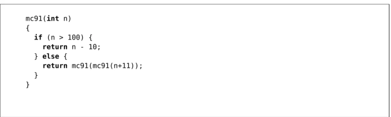
Another example shows that some properties can be more difficult to discover
automat-ically. Consider the code in Figure 1.
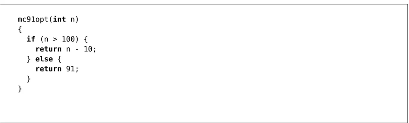
mc91(int n) { if (n > 100) { return n - 10; } else { return mc91(mc91(n+11)); } }
mc91opt(int n) { if (n > 100) { return n - 10; } else { return 91; } }
Figure 2: McCarty’s 91 function
This famous function has the following property:
mc91
(n) =
n − 10,
ifn > 100
91,
otherwiseHence, the function can be transformed in the more efficient version in Figure 2.
However, the transformation from mc91 to mc91opt requires finding a property that is
difficult to obtain from the code of the function. Running LLVM and GCC optimizers don’t
lead to the removal of the recursion.
This example demonstrated that the scope of the optimizations can still be enhanced
by finding additional information and properties about the code. This corresponds to the
intuitive principle that if the compiler “gets to know” more about the input program, it can
obtain better optimized code. In order for the compiler to know more, one can think of two
•
Refine further the compiler analysis•
Convey additional information from external sourcesCompiler theory focused on the first solution. Although this approach delivered very
good result, it’s far from finding all the interesting properties of a program (where
“inter-esting” means properties that can lead to an optimization).
Consider the case where some properties are computed by an external static analyzer
(e.g. an analyzer combined with an SMT solver) or given by a human (for example, the
pro-grammer writing the contract of a function). The aim of the thesis is to build a framework
that can exploit this additional information so as to broaden the scope of the optimization.
Since the optimization process is composed of different transformation passes, it is
necessary that the additional information can be used by any of the transformations, and
furthermore that the information is still correct after the previous transformations. This
is not a trivial problem, since some optimization passes may modify the structure and
the control flow of the source program, thus invalidating the invariants. In order to be
propagated throughout a transformation pass, an invariant might be modified to preserve
its validity. To solve this problem the thesis describes the concept of witness generator to
check the validity of the transformation and to carry the invariants from the source to the
target program. The generated witness can then be checked independently to prove the
correctness of the output; having an independently verifiable proof of the correctness of a
1.1 Problem definition
The thesis aims to solve three different, yet intertwined, problems. More precisely, the
problems are in a consequential order, i.e. by solving the first one the second arises, and
by solving the second one the third arises:
a) How to augment the scope and the quality of the optimization?
b) How to propagate assertions from end to end of an optimization pass?
c) How to check the correctness of the transformation and the propagation?
1.1.1 How to augment the scope and the quality of the optimization
As stated before, this work tries to solve this problem by conveying additional
informa-tion from external sources. Thus the problem can be reformulated in another way: “how
to let the compiler understand additional information to be used to augment the scope and
the quality of the optimization?” If we think, for example, hand-inserted annotations within
the code, like JML specification for Java, it could be useful for the optimization, if these
assertions are proven correct, to use them as additional information. The annotations are
usually written in a first order logic-like language.
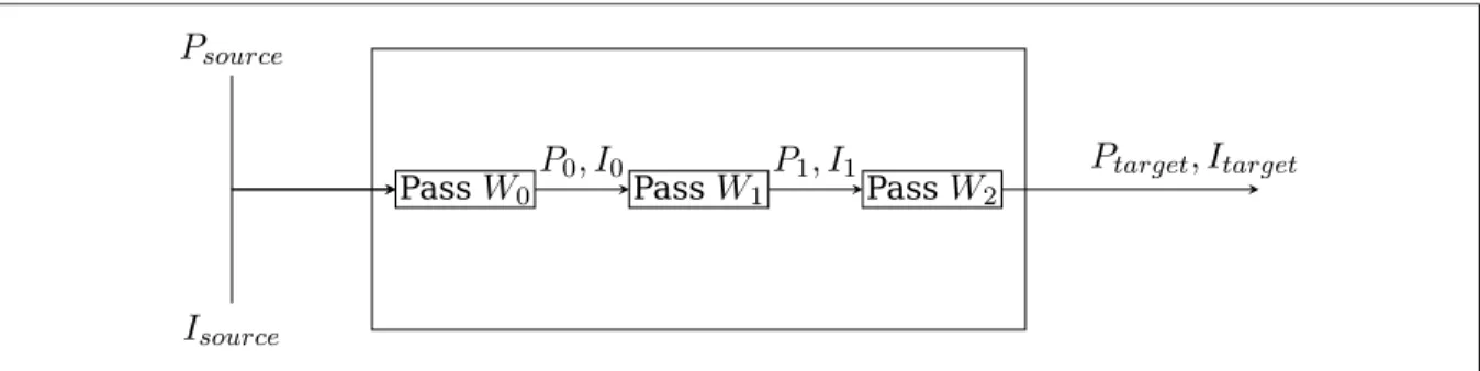
1.1.2 How to propagate assertions from end to end of an optimization pass Let
P
source be a program to be optimized andP
target the output program of theopti-mization pass, which is equivalent to
P
target. LetI
source be a set of properties ofP
source.The problem is to find a set of properties
I
target valid inP
targetthat are equivalent in someT : P → P
, whereP
is the set of all programs, such thatP
target= T (P
source)
. To solve theconsidered problem, the transformation definition is modified in this way: a transformation
W
is a functionW : (P × I) → (P × I)
, whereI
is the set of all sets of properties aboutprograms, such that
(P
target, I
target) = T (P
source, I
source)
.1.1.3 How to check the correctness of the transformation and the propagation The formulation of problem in Section 1.1.2 leads to the problem on how to formulate
an automatic checker that verify that, given that the properties about the source program
are correct:
a) The target program is equivalent to the source program
b) The soundness and correctness of the properties is preserved in the target program
For point a) different approaches are described in literature of formal methods and
compilers. Naively proving correctness of a transformation over all legal inputs, as
con-ducted in[2], is obviously infeasible most of the times. An alternative way of certifying each
instance is translation validation ([3],[4]), which employs heuristics to guess a witness for
every instance of a sequence of unknown transformations. The use of heuristics, however,
limits its applicability. Besides the drawbacks described above, these two solutions don’t
offer any method to deal with point b).
Such joint problems don’t find a solution in the current approaches, hence the need of
P
sourceI
sourcePass
W
0 PassW
1 PassW
2P
0, I
0P
1, I
1P
target, I
targetFigure 3: Overall architecture
1.2 Proposed solution
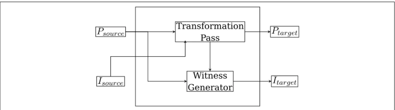
This thesis presents a framework to solve the problems stated above. The architecture
is designed around that of a standard optimizing compiler, which consists of a sequence of
optimization passes. Every pass takes as input a program, conducts its own analysis of the
program (possibly making use of information gathered in earlier passes), and produces a
program as output, optimized according to some metric (computation time, space, energy,
etc.).
We build upon this basic architecture by augmenting each analysis pass so that it
cor-rectly transmits the information obtained initially from annotations to all passes. As each
pass may arbitrarily transform its input program, it is necessary to transform the
informa-tion as well in order to retain its usefulness for subsequent passes (Figure 3).
To obtain this result, the existing optimizations are modified in two ways. First,
trans-formation passes are built to understand the annotations passed externally and use them
can use. A Witness Generator is built for every optimization; the witness Generator
gener-ates a witness that can be proved independently to check the validity of the transformation
(Figure 4).
The approach for generating the witness is to set a stuttering simulation relation
be-tween source and target programs. Stuttering simulation, as defined in[5], in this context
comes more useful than regular strict simulation, as the target program may have fewer
instructions than the source. It is shown[3] that establishing a stuttering simulation
re-lation from target to source is a sound and complete method for proving correctness, as
opposed to strict simulation.
The framework is built upon the Low-Level Virtual Machine compiler (LLVM). The
choice is driven by the fact that LLVM represent a state of the art, modern, modular
com-piler, with a well maintained and documented codebase. LLVM optimization passes work
on an intermediate language called LLVM Intermediate Representation (IR), as presented
in[6]. The IR is a Static Single Assignment (SSA) based representation that provides type
Transformation Pass Witness Generator
P
sourceP
targetI
sourceI
targetsafety, low-level operations, flexibility, and the capability of representing “all” high-level
languages cleanly. It is the common code representation used throughout all phases of the
LLVM compilation strategy.
This work is structured as follows. Chapter 2 introduces the concepts of witness and
invariant propagation. They will be analyzed from a formal point of view, and some key
properties of the witness are demonstrated. It is described that stuttering simulation is
a sound and complete witness relation for generic code transformation, and that the very
witness relation can be used to propagate the invariants. In Chapter 3 the theoretical
con-cepts shown previously are applied to some common optimizations in order to exemplify
the critical points. For every optimization presented, a corresponding witness is described.
In Chapter 4 the design of the actual framework is presented and the key details of the
implementations are described. It also describes how the transformations presented in
the previous chapter are implemented. Chapter 5 describes the results obtained by the
framework and the goals that will be pursued in the future, as well as provide with a
con-clusive overview of the work, comparing it to some related researches, and it introduces
THE TRANSFORMATION WITNESS
2.1 Introduction
To carry the annotations from the source program to the target, a witness relation is
built for every transformation. The generated witness is also used to check the
correct-ness of the transformation, since it can be verified independently from the transformation.
This makes the witness a very convenient and powerful abstraction, because proving its
correctness is simpler than proving the formal correctness of a transformation, that is
gen-erally very complex. In a modern compiler, for example, even the simplest transformation
can be made up of thousands of line of code. Witnessing a transformation is a new idea in
the field of formal methods and compilers, and as such, it needs a formal definition that can
be used in the theorems and hypotheses about its properties. From a theoretical point of
view, the layout of witness generation is simple, yet, defining and proving its completeness
requires some non-trivial demonstrations. In this chapter the concept of stuttering
simu-lation is also introduced, and it is shown that establishing a stuttering simusimu-lation resimu-lation
from target to source is a sound and complete method for proving correctness.
The theory that is being presented inside this chapter was developed by Zuck and
Namjoshi, in the paper called “Witnessing Program Transformations”[7]. A briefer
ap-proach is given in[8], where the results of this work are summarized.
2.2 Definitions
The definitions presented in this section are basically the one used in[7], with some
minor changes to fit the implementation.
Definition 1 Program
A program is described as a tuple
(V, G, T, I)
, where• V
is a finite set of (typed) variables• G
is a finite directed graph (it can be, for example, the control-flow graph)• T
is a function specifying, for every edge(i, j) ∈ G
, a symbolic transition conditiondenoted
T
i,j(V, V
0)
. Primed variables are used to denote the value of the programvariables at the program state after the transition
• I(V )
is an initial condition for the programEvery transition relates current and next-state values of the variables.
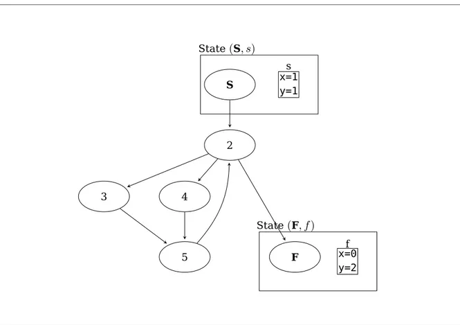
G
has twodis-tinguished nodes, S and F. The S node has no incoming edges, and the F node has no
outgoing edges, meaning that from
F
no transition can be triggered (see Figure 5). In thiswork we assume that every program P is deadlock-free, meaning that only the node F has
no enabled outgoing transition.
A state of a program is given by a pair
(l, v),
wherel
is a node ofG
andv
istype-consistent assignment of values to each variable in
V
. A state is defined as initial if andonly if
l =
S∧ I(v)
holds. A state is final if and only ifl =
F.S 2 4 3 5 F x=1 y=1 x=0 y=2 s f State
(
S, s)
State(
F, f )
Figure 5: Example of graph
G
. A pair(l, v)
is a state. State(
S, s)
is initial, State(
F, f )
is finalDefinition 2 Transition System
A transition system
T
is given by a tuple(S, I, R)
where:• S
is a set of states,• I
is the subset of initial states (i.e. inputs),A program
P (V, G, T, I)
(as definied in Definition 1) induces the transition system wherethe states are interpretations of
V
, the initial states are the those inI
, and the relationR
is that defined symbolically by
T
. Using the definition of transition system instead of theprogram in the simulation definition will simplify them, without losing generality.
Moreover, a program computation of lenght
n
is a sequence of statess
0, s
1, . . . s
nwheres
0 is initial and for each pairs
i= (l
i, v
i), s
i+1= (l
i+1, v
i+1)
of consecutive states on thesequence,
(l
i, l
i+ 1)
is an edge inG
, and the transition conditionT
i,i+1(v
i, v
i+ 1)
holds.A computation can have infinite length. A computation is terminating if
s
n= (
F, v
n)
. Acomputation is maximal when no transition can be enabled from the last state, i.e., when
it’s terminating or infinite.
Definition 3 State Matching
Let
T
,S
be two programs andT
T(S
T, I
T, R
T)
,T
S(S
S, I
S, R
S)
the corresponding transitionrelations. States
t ∈ S
T ands ∈ S
S match, denotedt ' s
, ift
ands
assign the same valueto every variable
v ∈ V
0= V
S∩ V
T.Definition 4 Path Matching
For Programs
T
andS
a maximal computationτ
of programT
is matched by a maximalcomputation of
σ
of programS
if the following conditions all hold:•
The starting state ofT
andS
match•
if(
FT, v) ∈ τ
for some variable assignmentv
, then for somew
,(
FS, w) ∈ σ
Definition 5 Implementation
Given two programs,
T
andS
,T
implementsS
if for every maximal computationτ
ofT
,there is a maximal computation
σ
ofS
that matches it.If
T
implementsS
, then every terminating computation ofT
has a correspondingter-minating computation of
S
starting from a matching initial state such that the final states(if any) also match. Hence, the input-output relation of
T
is included in that ofS
, w.r.t.the common variables. Moreover, if
T
has a non-terminating computation from someini-tial state, non-termination is also possible for
S
from a matching state. This disallows, forexample, pathological “implementations” where
T
has no terminating computations, sothat the input-output relation of
T
(the empty set) is trivially contained in the input-outputrelation of
S
.Definition 6 Transformation Function
A transformation is a partial function on the set of programs. A transformation
δ
is correctif for every program
S
in its domain,T = δ(S)
implementsS
.In practical terms, a transformation is partial because it needs not to apply to all
pro-grams. Indeed, much of the effort in compiler optimization is on the analysis required to
determine whether a particular transformation can be applied. This is a very important
point, that enforces the idea that, from a theoretical point of view, verifying the witness is
much easier than verifying the whole transformation. It should be remembered also that
all legal inputs. As translation validation approach[9], the witness aims at verifying that an
instance of transformation produced an output that implements the input.
2.3 Simulation relations
Now we introduce two different kind of transition relations: Step and Stuttering
Simu-lation. Both of them can be used as witness format, since, as it will be pointed out below,
both can guarantee that the target program is a correct implementation of the source. The
basic difference between the two relations is in terms of the kind of transformation that
can be witnessed. A proof of the properties of the simulation is sketched but not formally
expressed. The complete demonstrations are laid out in[7].
Definition 7 Step Simulation
Given the transition systems
T
andS
, a relationX ⊆ S
T× S
S is a step simulation if:•
the domain ofX
includes all initial states ofT
•
for any(t, s) ∈ X
,t
ands
satisfy the same propositions and for everyt
0 such thatt, t
0∈ R
T, there is as
0such that(s, s
0) ∈ R
Sand(t
0, s
0) ∈ X
.It is shown in[7] that step simulation guarantees that the target program is a correct
implementation of the source:
Theorem 1 Step Soundness[7]
For programs
T
andS
,T
implementsS
if there is a step simulationX(S
S× S
T)
from thestates of every
T
-computation to the states ofS
-computation such that:•
for every final statet
T ofT
, if(t
T, t
S) ∈ X
thent
S is a final state ofS
Thus, checking the single-transition conditions of step simulation, together with the
two additional conditions of Theorem 1, is enough to show that
T
implementsS
. Thesechecks can be encoded as correctness questions and resolved with an automatic decision
procedure.
However, it is not always possible to draw a transition relation between a correctly
implemented target and its source program. In fact, if a step simulation relation can be
defined, for every step taken in the target transition, there is a corresponding step in
the source transition. This obviously requires the two transitions to have the same exact
length.
Stuttering Simulation Relation, the next witness format that is described, relaxes this
exact, 1-1 matching by permitting
τ
andσ
to be matched in segments, as illustrated inFigure 6.
τ
σ
It has been demonstrated[5] that the segments can be replaced by single steps, adding
an additional dimension to the stuttering simulation relation. This is done by adding a
ranking function
Rank : (T, S) → N
which decreases strictly at each stuttering step. Inthis work a simpler form of stuttering simulation is necessary.
t
t
0s
s
0X
X
(a) Case 1t
t
0s
s
0X
X
V
≺
(b) Case 2t
t
0s
X
X
≺
(c) Case 3Figure 7: Stuttering Simulation with ranking
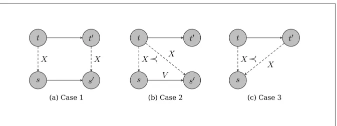
Definition 8 Stuttering Simulation with Ranking function
Given Transition systems
B
andA
, a relationX ⊆ S
T× S
S augmented with a partialranking function,
Rank : (S
T, S
S) → N
, over a well-founded domain(N, ≺)
, is a stutteringsimulation if:
•
for any(t, s) ∈ X
,t
ands
satisfy the same propositions and for everyt
0 such that(t, t
0) ∈ R
T, one of the following holds:– There is
s
0 such that(s, s
0) ∈ R
S∧ (t
0, s
0) ∈ X
(Figure 7a), or– There is
s
0 such that(s, s
0) ∈ R
S∧ (t, s
0) ∈ X ∧ rank(t, s
0) ≺ rank(t, s)
(stutteringon A, Figure 7b), or
–
(t
0, s) ∈ X
and rank(t
0, s) ≺ (t, s)
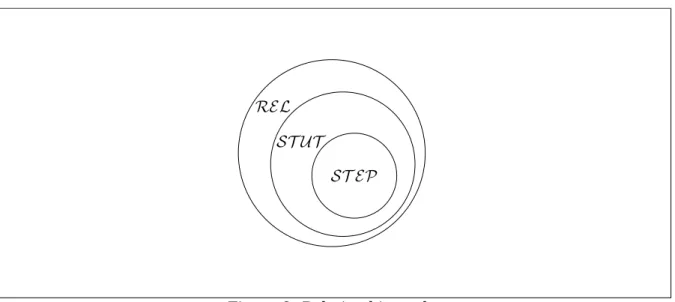
(stuttering on B, Figure 7c).A graphical explanation of this definition is given in Figure 7. It is immediate to
ob-serve how step simulation is a specialization of stuttering simulation. If we define three
sets
REL, ST U T , ST EP
as the set of all general relations, step simulation relations andstuttering simulation relations respectively, we have
ST EP ⊂ ST U T ⊂ REL
(Figure 8).This result will help to clarify some considerations. While
REL
can define everytransfor-mation relation from program
A
toB
, not all are correct (i.e,B = X(A)
implementsA
). Onthe other hand, this is true for all the step simulations (Theorem 1), yet, as already stated
before, step simulation is too restrictive in terms of transformations that can be simulated.
In fact, it can be applied only when the the transformation doesn’t rearrange, eliminate or
add instructions. Therefore, stuttering simulation is the best candidate to accommodate all
kind of transformations, as it is, we’ll observe, a sound and complete simulation. It must
be considered also that the definition of stuttering simulation adds an additional
dimen-sion to the relation, that is the one defined by the ranking function that accompanies the
figure doesn’t take into account the ranking function, so it is a simplification of the actual
property of stuttering simulation. In fact, as it is shown in[7], without the ranking function
it wouldn’t be possible to demonstrate the completeness of the stuttering simulation.
REL
ST U T
ST EP
Figure 8: Relation hierarchy
Theorem 2 Soundness[7]
Let
X
be a stuttering simulation relating states of a programT
to those of programS
.Then
T
is a correct implementation ofS
when the following conditions all hold:•
For every initial states
ofS
, there is an initial statet
ofT
such that(t, s) ∈ X
and•
Final states ofS
orT
areX
-related to only final states of the other program.More-over, if
t
ands
areX
-related final states ofT
andS
, thent ' s
.The conditions expressed in the soundness theorem gives the definition of Witness
Relation:
Definition 9 Witness
Let
S
andT
be programs related by a stuttering simulation relationW
from the state spaceof
T
to that ofS
.W
is a Witness relation if the soundness conditions hold:•
For every initial stateu
ofT
, there is an initial statev
ofS
such that(u, v) ∈ W
andu ' v
.•
Final states ofS
orT
areW
-related to only final states of the other program.More-over, if
u
andv
areW
-related final states ofT
andS
, thenu ' v
.In other words, that means that the stuttering simulation is a sound witness.
Based on Manolios[10], Namjoshi and Zuck proved that stuttering simulation is sound
and complete.
2.4 Invariant propagation
A relation that satisfies the Witness format can also be used to “propagate” the
asser-tions from end to end of the transformation pass, making the additional transformation to
be used also in different part of the transformation process, rather than just by the first
section. Propagation informally means that if an assertion
θ
is true for a subset of sourcestates
S
0S∈ S
S, the propagated assertionθ
0 must be true for all and only the target statesS
T0∈ S
T where every statet ∈ S
T0 is related to some states ∈ S
S0 by the witness relationW
. Now a more formal description will be provided.First we define the concept of pre-image of
θ
underW
, denoted (hW iθ
), as the set{(m, t)|(∈ l, s : ((m, t), (l, s)) ∈ W ∧ θ(l, s)}
. The following theorem holds:Theorem 3 Invariant Propagation[7]
Let
W
be a stuttering simulation witness for a transformation from programT
to programS
. Ifθ
is an invariant forS
, the sethW iθ
is an invariant forT
. Moreover, ifθ
is inductive,so is
hW iθ
.The sketch of the proof for the correctness of
hW iθ
as invariant at Target is as follows.Let
θ
be an invariant holding for every state of a programS
. For every valid computationτ
of programT
, there must exist, from the definition of witness relation, a computationσ
of program
S
such that∀t ∈ τ, ∃s ∈ σ, W (t, s)
. It is true also that∀s ∈ σ, s ∈ θ
. The lastformula holds because
σ
is a computation of S (whereθ
holds). Combining the last twoformulas ensues that
S
t∈τ
∈ hW iθ
. Hence,hW iθ
is a correct invariant for programT
.2.5 Generalization
The transition relation can be generalized and adjusted to the concept of control-flow
graph (CFG) of a program
P
. In this generalization, the states of a program refers only tothe beginning of a basic block of the graph, and the transition relation maps every node
one instruction. The generalization is useful for two different reasons. This restricts the
cases where step simulation is not sufficient and stuttering simulation is necessary,
Consider the example of Dead Code Elimination. As it will be shown in the following
chapter, DCE transformation can be witnessed by a stuttering simulation relation.
How-ever, if we generalize the transition relation to work over the basic blocks rather than
single instructions, step simulation is sufficient to prove the correctness of this
transforma-tion. This is due to the fact that Dead code elimination doesn’t change the CFG structure.
Hence, it follows that stuttering simulation is usually necessary when the transformation
reorders, eliminates, or add nodes of the Control Flow Graph.
The second reason is that many compilers, such as LLVM, build the CFG of the
func-tion as a preliminary step before every optimizafunc-tion pass. This implies that building the
generalized relations over the existing CFG is a more efficient approach than building
WITNESS FOR COMMON OPTIMIZATIONS
In this Chapter the witnesses for several standard optimizations are defined. These
optimizations are chosen for their commonality and in order to illustrate features of the
witness generation. We consider constant propagation, dead code elimination, control-flow
graph compression and loop optimizations.
Some transformations can be witnessed with a simple step simulation, however other
transformations require the simulation to be stuttering, as the transformation can result
in the target being shorter or longer than the source. As a side result of the examples, it
is shown that the analysis required to check if a transformation can be triggered is more
difficult than the witness generation procedure, showing that witness generation can be, in
theory, an efficient transformation checker. Witness generation, essentially, makes explicit
the implicit invariants gathered during the analysis. These examples confirm also the
concept that, from a theoretical point of view, a witness can be generated for every kind of
optimization, even though the complexity of the optimization will impact on the complexity
of the witness. The examples are taken from[7], and modified to highlight the details that
this chapter wants to stress out.
The actual implementation for some of these transformations will be exposed in
Chap-ter 4. Therefore all the details concerning the implementation will be put aside, in order
to focus on the key concepts both of witness generation and invariant propagation. 23
L1: x = 1+2; L2: y = x+x; L3: y = y+1; L4: x = y; (a) Source L1: x = 3; L2: y = 6; L3: y = 7; L4: x = 7; (b) Target
Figure 9: Constant propagation example
3.1 Constant Propagation
In the Constant Propagation pass, the analysis checks if any variable has a static
as-signed constant value. In the example of Figure 9 all the values are constant-folded up.
The witness generation for constant propagation basically draws from the invariants
generated during the analysis. The invariant, called
constant(l)
, simply describes the setof variables that have a statically computed constant value at location
l
. For example, theinvariant at L3 is
x = 3 ∧ y = 6
.The witness relation is expressed in a symbolic form. The general shape of the relation
for constant propagation is the following: a target state
(m, t)
is related to a source state(l, s)
if and only if:•
labels are identical (i.e.,m = l
),•
variables have identical values (i.e., for every variablex, s(x) = t(x)
), and•
variables in the source system have values given by their invariant (i.e.,constants(l)
Where for every variable
x
in the source,x
¯
indicates its corresponding version in thetarget. For example, in symbolic form, the relation includes the clause
@L3 ∧ @ ¯
L3 ∧ (x = ¯
x) ∧ (y = ¯
y) ∧ (z = ¯
z) ∧ x = 3 ∧ y = 6
It’s necessary that the invariants hold at the source location, because this establishes
the correspondence between target and source. For instance, the transition from
L2
toL3
is matched by the transition fromL2
¯
toL3
¯
only because the value ofx
is defined asconstant in
constant(L2)
3.2 Dead Code Elimination
Dead code elimination analyzes the code, building use-define chains for every
assign-ment instruction, and marks all those instructions for which use set is empty. This means
that the assigned value is not being used in any of the program computation and removing
it doesn’t change the semantics of the code. In this context, dead code elimination is split
in two separate phases, the second being a restrictd instance of control flow graph
com-pression. If the transition from location
m
to locationn
assigns a value to a variablev
thatis dead (i.e., not live) at
n
, this assignment may be replaced with a skip statement. This isillustrated in Figure 10 which performs dead-code detection for the output of the constant
propagation analysis. The result of the liveness analysis is a set, denoted
live(l)
, for eachL1: x = 3; L2: y = 6; L3: y = 7; L4: x = 7; (a) Source L1: x = skip; L2: y = skip; L3: y = 7; L4: x = 7; (b) Target
Figure 10: Dead code elimination example
Here is described a general procedure for generating a witness for DCE. A target state
(m, t)
is related to a source state(l, s)
if and only if:•
labels are identical (i.e.,m = l
), and•
every variable that is live atl
has the same value as the corresponding variable atm
.I.e., for every variable
x
such thatx ∈ live(l) : s(x) = t(x)
.For example, in symbolic form, the relation includes the clause
@ ¯
L4 ∧ @L4 ∧ (y = ¯
y)
as only the variable
x
is live atL4
. For any correct dead code elimination transformation,the relation defined above is a strong simulation witness.
Continuing the example from the result of dead code elimination, the control flow
L1: x = skip; L2: y = skip; L3: y = 7; L4: x = 7; (a) Source L3: y = 7; L4: x = 7; (b) Target
Figure 11: Control-Flow-Graph compression example
skip; S → S
, for any statementS
. This compresses the control flow graph. Other instancesof compression may occur in the following situations:
•
a sequence such as goto L1; L1:S is replaced with L1:S, or•
the sequence S1; if (C) skip else skip; S2 is replaced with S1;S2.In all these cases the computation in the target is shorter than the one in the source,
The general witness definition relates a target state
(m, t)
to a source state(l, s)
ifs = t
and either
l = m
orl
lies on a linear chain of skip statements fromm
in the source graph.For a correct control-flow graph compression, the defined relation is a stuttering
sim-ulation witness. Moreover, as a result of the closure property for stuttering simsim-ulation,
it is possible to take the witnesses for constant propagation
W
1, dead-code eliminationW
2, and control-flow graph compressionW
3 and compose them to form a single witnessW = W
1; W
2; W
3for the transformation from the program in Figure 9a to the program in3.3 Reordering Transformations
A reordering transformation is a program transformation that changes the order of
ex-ecution of the code, without adding or deleting any statements. It preserves a dependence
if it preserves the relative execution order of the source and target of that dependence, and
thus preserves the semantical meaning of the program. Reordering transformations cover
many loop optimizations, including fusion, distribution, interchange, tiling, and reordering
of statements within a loop body.
A generic loop can be described, as introduced in[3], by the statement for
i ∈ I
by≺
Ido B(i) where
i
is the loop induction variable andI
is the set of the values assumed byi
through the different iterations of the loop. The set
I
can typically be characterized by a setof linear inequalities. While in[3] “structure preserving” and “Reordering” transformation
passes are treated differently, here we follow[7] and let the witness relation to be defined
so that it allows for uniform treatment of the two types of transformations.
3.4 Loop Invariant code motion
Loop invariant code motion (also referred to as “hoisting”) moves some instructions
from the inner to the outer body of a loop without affecting the semantics of the program.
Usually a reaching definitions analysis is used to detect whether a statement or expression
is loop invariant. For example, if all reaching definitions for the operands of some simple
assignment are outside of the loop, the assignment can be moved out of the loop. Moreover,
in order to move instructions outside the loop, LICM analysis must guarantee that there is
L0: i = 1; L1: while(i<100){ L2: c = 3; L3: i = i + 1; } (a) Source L0: i = 1; L2: c = 3; L1: while(i<100){ L3: i = i + 1; } (b) Target
Figure 12: Loop Invariant Code Motion example
Figure 12 which is a simplified version of an example from[11]. Since the loop is going to
be executed at least once, the assignments to
a
andc
, which are not dependent on anystatement in the loop body, can be moved outside of the loop.
The transformation analyzer will detect the lack of dependencies of the statement in
L2
on the other statements in the body, together with the fact that the loop is guaranteedto be executed at least once. The witness is generated in the following fashion. The
simulation maps the first statements of the target program (In this case
L0
) and the firstiteration of the target loop into the first iteration of the source loop. This mapping of course
stutters, as there are more instructions in the target program segment than in the source
program segment. Thus, the corresponding symbolic (stuttering simulation) will include
the following clause:
L3 ∧ ¯
L3 ∧ i = ¯i ∧ c = ¯
c ∧ c = 3
. From the second iteration onwards,when
i > 1
, the two loops are linked one by one in a stuttering simulation (since one targetThere is also a more general Loop invariant code motion that combines “hoisting”
(where the instructions are moved before the loop body, as seen above) and “sinking”
(where the instructions are moved after the loop body). For sinking, it must be checked
that the moved instruction is not used inside the loop and that the loop is executed at least
once. Given that, the witness generation follows the one described for the hoisting loop
DESIGN AND IMPLEMENTATION
In this chapter we describe the implementation of the theoretic transformations
de-scribed in Chapter 2: witness generation, witness checking and invariant propagation.
The source code is available as a git repository1. Basically it is a fork from the original
LLVM repository where the additional passes and structures are being added. Description
on how to run the program and basic examples are given in Appendix A.
We introduce an overview of the technologies being used, particularly LLVM and Z3.
These are open-source projects, the source code is downloadable from their respective
websites2 3.
4.1 LLVM
LLVM (Low-Level virtual machine) is a compiler that provides a modern source- and
target-independent optimizer, along with code generation support for many popular CPUs.
These libraries are built around a well specified code representation, known as the LLVM
intermediate representation ("LLVM IR"). The LLVM Core libraries are well documented,
1https://bitbucket.org/itajaja/llvm-csfv
2LLVM website: llvm.org
3Z3 website: z3.codeplex.com
they present a very modular and understandable code and offer various tools to help the
programmer in using them.
A fundamental design feature of LLVM is the inclusion of a language-independent type
system, namely LLVM Intermediate Representation (IR ). The LLVM representation aims
to be light-weight and low-level, while being expressive, typed, and extensible at the same
time. It aims to be a “universal IR”, by being at a low enough level that high-level ideas may
be cleanly mapped to it. By providing type information, LLVM can be used as the target of
optimizations: for example, through pointer analysis, it can be proven that a C automatic
variable is never accessed outside of the current function, allowing it to be promoted to a
simple SSA value instead of a memory location.
The LLVM IR can be represented in three equivalent forms:
•
As in-memory data structure•
As Human readable Assembly-like text format•
As a bytecode representation for storing space-optimized and fast-retrievable filesLLVM is able to convert consistently and without information loss from one form to
another, depending on the result one wants to achieve. LLVM optimizer accepts any of
these three forms as input, then, if the input is in assembly or bytecode form, it converts it
in the in-memory format to perform the optimizations, and then it can reconvert it in one
of the requested three forms. Additionally, it can call the back-end driver to convert the IR
LLVM programs are composed of Modules, each of which is a translation unit of the
input programs. Each module consists of functions, global variables, and symbol table
entries. Modules may be combined together with the LLVM linker, which merges function
(and global variable) definitions, resolves forward declarations, and merges symbol table
entries. Listing 4.1 shows the code for the HelloWorld Module.
; ModuleID = ’hello.c’
target datalayout = "e-p:64:64:64-i1:8:8-i8:8:8-i16:16:16-i32:32:32-i64:64:64-f32:32:32-f64 :64:64-v64:64:64-v128:128:128-a0:0:64-s0:64:64-f80:128:128-n8:16:32:64-S128"
target triple = "x86_64-pc-linux-gnu"
@.str = private unnamed_addr constant [14 x i8] c"Hello World!\0A\00", align 1 define i32 @main(i32 %argc, i8** %argv) nounwind uwtable {
%1 = alloca i32, align 4 %2 = alloca i32, align 4 %3 = alloca i8**, align 8 store i32 0, i32* %1
store i32 %argc, i32* %2, align 4 store i8** %argv, i8*** %3, align 8
%4 = call i32 (i8*, ...)* @printf(i8* getelementptr inbounds ([14 x i8]* @.str, i32 0, i32 0))
ret i32 0 }
declare i32 @printf(i8*, ...)
Listing 4.1: Example of IR code
In LLVM (as in many other compilers) the optimizer is organized as a pipeline of distinct
code. Common examples of passes are the inliner (which substitutes the body of a function
into call sites), expression re-association, loop invariant code motion, etc. Depending on
the optimization level, different passes are run: for example at -O0 (no optimization) the
Clang front-end for C program runs no passes, at -O3 it runs a series of 67 passes in its
optimizer (as of LLVM 2.8).
Each LLVM pass is written as a C++ class that derives (indirectly) from the Pass class.
Most passes are written in a single .cpp file, and their subclass of the Pass class is defined
in an anonymous namespace (which makes it completely private to the defining file). An
example of pass is given in Listing 4.2
#include "llvm/Pass.h" #include "llvm/Function.h"
#include "llvm/Support/raw_ostream.h" using namespace llvm;
namespace {
struct Hello : public FunctionPass { static char ID;
Hello() : FunctionPass(ID) {}
virtual bool runOnFunction(Function &F) { errs() << "Hello: "; errs().write_escaped(F.getName()) << ’\n’; return false; } }; } char Hello::ID = 0;
static RegisterPass<Hello> X("hello", "Hello World Pass", false, false);
Every function pass overrides a runOnFunction() method, that will be run on every
function, and will perform customs analysis and transformation over the targeted piece of
code.
4.2 SMT solver
When the witness is generated, its correctness must be proved. The theory of formal
methods offers different techniques to prove the correctness of a formula against a
pro-gram representation. Especially, Satisfiability Theories (SAT ) and its extension
Satisfiabil-ity Modulo Theory (SMT ) allow to determine whether a given First order logic formula is
satisfiable or not with an arbitrary assignment of variables. While SAT solvers can handle
only boolean variables, SMT solvers can handle different logical theories. SMT solvers are
broadly used in formal methods to formally prove the correctness of a program given some
FOL constraints ([12],[13]) and several automated solvers has being proven to proficiently
solve difficult SMT problems.
4.2.1 Z3
Z3 is a widely employed SMT automated solver developed by Microsoft research, whose
code is freely available for academic research. It handles several different theories such
as empty-theory (uninterpreted function theory), linear arithmetic, nonlinear arithmetic,
bit-vectors, arrays and data types theory. Besides accepting user input at runtime, it
ex-poses interfaces for python, OCaml, Java, .NET languages, C and C++. The C++ APIs are
integrated in the ACSL Passes to generate and check the witness, as it will be described
We selected Z3 for its performance, number and quality of features (mostly in terms of
implemented theories), easiness to use. Moreover, its C++ API are concise,
understand-able, well documented and almost plug-and-play for all main platforms.
4.3 Overview of transformation passes
The current version of LLVM implements many analysis and transformation passes1,
from the basic common to the most highly engineered ones. They are roughly subdivided
into analysis, transformation and utility passes. Among the transformation passes, we can
count Dead Code Elimination, Constant Propagation, Sparse Conditional Constant
Prop-agation, Instruction Combine, Function Inlining, Loop invariant code motion, Loop
un-rolling, Loop Strengthen Reduction etc. Different optimizations can run at different layers
of the intermediate representation. Depending on its functionality, a pass can run on the
overall module, on each function, on each Basic Block, on each loop, or on each
instruc-tion. Herein the passes that are taken mostly in consideration are the function passes,
which are the most common ones and can perform significant optimizations. The passes
are then organized together by a Pass Manager that decides the order of execution of the
passes, and whether to re-execute a pass another time after the code has been changed.
The decisions are made based on a set of constraints, and they happen transparently from
implementing a new optimization. The following passes are chosen by their commonality,
ease of study and for clearly highlighting some of the critical parts of the framework.
4.4 ACSL Passes
In this section the design and implementation for the transformations listed in
Chap-ter 3 is described. We will refer to these transformations as “ACSL passes”1, to distinguish
them from the ordinary optimizations that don’t have witness generation. Some care is
needed while carrying the theoretical concepts and structures to an actual
implementa-tion: the abstraction layer where these objects are to be put doesn’t permit the concepts
to remain in a mathematical form, therefore there are some critical points that one must
take care of when translating from theory to practice.
The state, as defined in chapter 2, is “a pair
(l, v),
wherel
is a node ofG
andv
istype-consistent assignment of values to each variable in
V
”. Since, during static analysisis not always possible to assign a value to every variable, it won’t be possible to deal with
states as they are described in the definitions. In particular, because of the presence of
uncertainty about variable values, a program state may not necessarily correspond to a
unique state in the abstract program. Nevertheless, it suffices that the transition relation
(function) refers only the variables that have an assigned values. That is, being
x
a variablewith unassigned value, if the transition relation makes no reference to
x
, then it doesn’tmatter that
x
is not assigned a value. Therefore in the context of this work we explicitlychoose symbolic representation.
1The name refers to the annotation language, even if the transformation can be not directly related to ACSL at all. This name comes from a convention used before writing this work
The goal of the witness is to check if the target program implements the source, that is
to check whether or not the target program is a stuttering simulation of the source.
The process that has being followed to build an ACSL Pass is similar for every pass. The
starting base is the LLVM source, in particular, the code of the optimization that is going
to be implemented is modified to add the witness generator. First, the analysis phase
of the pass is augmented to store all the invariants found by the analysis in a way that
they will be able to be used by the witness. Every optimization will, of course, perform a
different analysis, and every result can be stored among the other invariants. The invariant
then is linked to a location in the code. If the invariant is the result of the analysis of a
single instruction, mapping the invariant to a location is effortless (the location will be
the analyzed instruction itself). If the invariant is the result of an analysis that involves
more than a single instruction, a location where the invariant holds has to be found, which
depends on the transformation pass. The witness generation phase follows the analysis
and the transformation passes. It construct a witness for each analyzed part of code. To
this end, is necessary to have the generated invariants, the source program relation and
the target program relation. Subsequently, the generated witness can be discharged to the
Z3 solver to check it satisfiability.
To carry the invariants from one pass to the next, we need a structure to preserve the
information gathered during the analyses as well as the one that is provided externally. The
class Invariant Manager exposes static methods to access a data structure where all the
exposes utilities to iterate over the annotations and to retrieve the invariant at a specified
location. It also keeps in memory the global values needed by the Z3 API to perform the
requested operations.
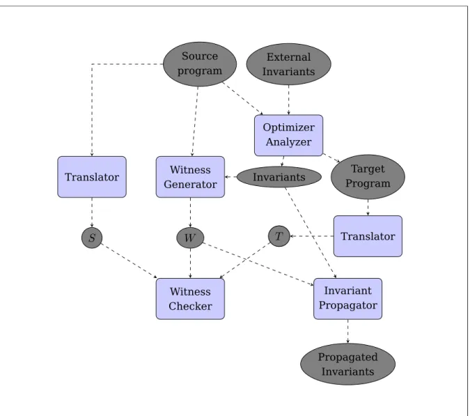
A generic work flow of the pass is given in Figure 13. The gray ellipses represents
objects and the teal boxes represent actions or components that takes the objects in input
that produces the objects in output. Now we analyze each basic component of the generic
Witness Generator Optimizer Analyzer External Invariants Source program Invariants Target Program
W
Witness Checker Translator TranslatorS
T
Invariant PropagatorT
Propagated InvariantsFigure 13: ACSL pass workflow
The Optimizer/Analyzer is where the transformation occurs. This component is
basi-cally the original LLVM transformation, it usually takes the Source Program and produces
Invariants as input and to produce, in addition to the source program, a list of Invariants
that is made up of the external invariants plus the eventual invariants found during the
analysis of the function.
The Witness Generator takes care of generating the transformation-specific Witness
Relation W. It takes as input the Invariants produced by the Analyzer and the Source
Program and traverses the source to produce the Witness Relation for the given program.
The produced output is a mathematical relation W in the state space of the program.
The Translator component transforms the LLVM intermediate representation into a
transition system. As described in chapter 2, the transition system is composed by a set
of states, a subset of initial states and a transition relation in the state space. For
conve-nience, the set of states is encoded as a propositional formula, which is a more convenient
form for the SMT solver. The translator takes as input both the source and the target
programs and produces two different relations, respectively S and T.
The Witness Checker is where the Witness Relation is tested against the target and
source transition system to see if it is a Stuttering Simulation (in some cases the step
simulation is enough, and it is more efficient to check the latter than the former). The
Checker relies on the Z3 solver to prove the satisfiability of the formula. If the witness
checker proved the transformation not to be correct, it will halt the optimization process
and produce an alert message.
If the witness checker proved the transformation to be correct, the Invariant
with the target program. The Invariants are produced calculating the pre-image of
θ
underW
(hW iθ
) as discussed in Chapter 2 . Z3 deals also of computing the propagatedinvari-ants. the set will be eventually stored in the Invariant Manager, substituting the former
set of invariant.
To summarize, the overall structure is as follows. For every optimization, there are two
outputs, source and external invariants, and two inputs, target and propagated invariants.
Every transformation pass has its own witness generator. The analysis phase needs to
be augmented to use the additional invariant input and produce new enriched invariants.
The translator, witness checker and invariant propagator are transformation-independent,
hence a single implementation of these component suffices to handle all the possible
trans-formations.
As stated at the beginning of Chapter 4, LLVM IR has three different representation.
The Invariant and Invariant Manager structures work with the in-memory representation
as all the LLVM transformation passes do. Thus, when the IR gets converted, it loses all the
annotations’ information, as there is yet no conversion functionality for the annotations.
Because of this limitation, the ACSL Passes are run at once before any other transformation
pass, then the annotations can be dropped and then the standard LLVM optimizations can
be run later, as they don’t make use of the additional information provided.
The current implementation of the annotation framework deals only with variables of
in-teger types, the transformation and the related examples described below will accordingly

![Figure 12 which is a simplified version of an example from [11] . Since the loop is going to](https://thumb-eu.123doks.com/thumbv2/123dokorg/7502321.104579/44.918.130.811.200.372/figure-simplified-version-example-loop-going.webp)