A pricing technique to calculate the solvency capital requirement for non-life premium risk

(1)

0 A pricing technique to calculate the Solvency Capital

Requirement for non-life Premium Risk

Department of Statistical Science

Andrea Tronconi

Tutor

(2)

1

2

CASE STUDY... 55

4.1 INTERNAL MODEL ... 55

4.2 SOLVENCY II STANDARD FORMULA ... 97

4.3 INCLUDING EXPENSES ...103

CONCLUSIONS ...107

(4)

3 INTRODUCTION

Figure 1: 1844-06-20 - Onondaga County Mutual Insurance Company – Policies.

Onondaga County New York Mutual Fire Insurance Co. 1844 policy, issued to Truman Woodford & Philip Alexander on June 1844. This policy is for coverage of Dwelling House & Barn. Handwriten name of town appears to be Tully located in the County of Onondaga.

“Each human activity is the result of a long chain of events, of the fate, opportunity, chances and the continuous modest work of millions of men: there is no human adventure which not involves risk”1_.

Early methods of transferring or distributing risk were practiced by Chinese and Babylonian traders as long ago as the 3rd and 2nd millennium BC, respectively. Chinese merchants travelling treacherous river rapids would redistribute their wares across many vessels to limit the loss due to any single vessel's capsizing. The Babylonians

(5)

4

developed a system which was recorded in the famous Code of Hammurabi, c. 1750 BC, and practiced by early Mediterranean sailing merchants. If a merchant received a loan to fund his shipment, he would pay the lender an additional sum in exchange for the lender's guarantee to cancel the loan should the shipment be stolen or lost at sea. Achaemenian monarchs of Ancient Persia were the first to insure their people and made it official by registering the insuring process in governmental notary offices. The insurance tradition was performed each year in Norouz (beginning of the Iranian New Year); the heads of different ethnic groups as well as others willing to take part, presented gifts to the monarch. The most important gift was presented during a special ceremony. When a gift was worth more than 10 000 Derrik (Achaemenian gold coin) the issue was registered in a special office. This was advantageous to those who presented such special gifts. For others, the presents were fairly assessed by the confidants of the court. Then the assessment was registered in special offices. The purpose of registering was that whenever the person who presented the gift registered by the court was in trouble, the monarch and the court would help him. Jahez, a historian and writer, writes in one of his books on ancient Iran: "Whenever the owner of

the present is in trouble or wants to construct a building, set up a feast, have his children married, etc. the one in charge of this in the court would check the registration. If the registered amount exceeded 10 000 Derrik, he or she would receive an amount of twice as much".

A thousand years later, the inhabitants of Rhodes invented the concept of the 'general average'. Merchants whose goods were being shipped together would pay a proportionally divided premium which would be used to reimburse any merchant whose goods were deliberately jettisoned in order to lighten the ship and save it from total loss.

The Greeks and Romans introduced the origins of health and life insurance c. 600 AD when they organized guilds called "benevolent societies" which cared for the families and paid funeral expenses of members upon death. Guilds in the Middle Ages served a similar purpose. The Talmud deals with several aspects of insuring goods. Before insurance was established in the late 17th century, "friendly societies" existed in

(6)

5

England, in which people donated amounts of money to a general sum that could be used for emergencies.

Separate insurance contracts (i.e., insurance policies not bundled with loans or other kinds of contracts) were invented in Genoa in the 14th century, as were insurance pools backed by pledges of landed estates. These new insurance contracts allowed insurance to be separated from investment, a separation of roles that first proved useful in marine insurance. Insurance became far more sophisticated in post-Renaissance Europe, and specialized varieties developed.

Some forms of insurance had developed in London by the early decades of the seventeenth century. For example, the will of the English colonist Robert Hayman mentions two "policies of insurance" taken out with the diocesan Chancellor of London, Arthur Duck. Of the value of £100 each, one relates to the safe arrival of Hayman's ship in Guyana and the other is in regard to "one hundred pounds assured by the said Doctor Arthur Ducke on my life". Hayman's will was signed and sealed on 17 November 1628 but not proved until 1633. Toward the end of the seventeenth century, London's growing importance as a center for trade increased demand for marine insurance. In the late 1680s, Edward Lloyd opened a coffee house that became a popular haunt of ship owners, merchants, and ships’ captains, and thereby a reliable source of the latest shipping news. It became the meeting place for parties wishing to insure cargoes and ships, and those willing to underwrite such ventures. Today, Lloyd's of London remains the leading market for marine and other specialist types of insurance, but it works rather differently than the more familiar kinds of insurance.

Insurance as we know it today can be traced to the Great Fire of London, which in 1666 devoured more than 13 000 houses. The devastating effects of the fire converted the development of insurance "from a matter of convenience into one of urgency, a change of opinion reflected in Sir Christopher Wren's inclusion of a site for “the Insurance Office” in his new plan for London in 1667." A number of attempted fire insurance schemes came to nothing, but in 1681 Nicholas Barbon and eleven associates, established England's first fire insurance company, the “Insurance Office for Houses”, at the back of the Royal Exchange. Initially, 5 000 homes were insured by Barbon's Insurance Office.

(7)

6

The first insurance company in the United States underwrote fire insurance and was formed in Charles Town (modern-day Charleston), South Carolina, in 1732. Benjamin Franklin helped to popularize and make standard the practice of insurance, particularly against fire in the form of perpetual insurance. In 1752, he founded the Philadelphia Contributionship for the Insurance of Houses from Loss by Fire. Franklin's company was the first to make contributions toward fire prevention. Not only did his company warn against certain fire hazards, it refused to insure certain buildings where the risk of fire was too great, such as all wooden houses.

It’s clear that one of the key elements of insurance is security, but what would happen if the insurance company is unable to pay the cost of the claim?

In this context, the solvency of insurance company is fundamental.

The pioneering works done by Cornelis Campagne in the Netherlands at the end of the 1940s and by Teivo Pentikäinen in Finland in the beginning of the 1950s are important, as they introduced the solvency research for insurance undertakings. Before the term solvency was introduced, a concept like statutory reserves was often used, which have been formed in the course of years and which serve as an extra guarantee for fulfilling the obligations undertaken. Initially, Campagne called this type of reserve for life insurance for a stabilization reserve. In Finland a special equalization reserve was introduced in 1953 to take account of the stochastic fluctuations in the annual claims amount in non-life insurance. During the 1950s Campagne enlarged the solvency assessment to non-life insurance. As Campagne’s work became leading for the approach of assessing an extra minimum reserve for both life and non-life companies he was asked to present a report on solvency (“Minimum Standards of Solvency for

Insurance Firms”) in 1957 to the OEEC2_{Insurance Committee. As a chairman of a}

working group within the Insurance Committee his work was developed and a final report was presented in 1961.

In life insurance the approach adopted was the same as in the 1940s. As the risk on investments is the most important factor for life insurance companies and as the technical provisions are the most important invested amount, Campagne considered a

(8)

7

minimum solvency margin as given by a percentage of the technical provisions. Campagne asked “how great has the extra reserve to be, so that with a probability smaller than 0.01 respectively 0.001 this can be expressed to be insufficient for the financing of investment losses and deviations of foundations; in which case furthermore distinctions have to be made between cases in which the stabilization reserve has to be sufficient for one year or more years.”. Campagne concluded that an extra reserve of 6% of the technical provision would be adequate with a probability of 99%.

With a probability of 95% the percentage of the extra reserve became 4% and this was the extra reserve proposed by Campagne. It was implemented in the first life directive within the European Union in 1979.

In non-life insurance the model was simple but elegant. Let the net retained premium

be 100%. From this we deduct a constant fraction equal to the average expense ratio3

(fixed to 42%). The remaining part is what remains for claims payment. With data from

different European countries he estimated the Value-at-Risk4_{of the loss ratio at}

0.9997% as 83%. Thus the combined ratio5 _{will be 42% + 83% =125%. In other words}

the company will need an extra 25% of the premium during 1 year to meet the requirements. After further works during the 1960s and political negotiations this framework became the base for the first non-life directive in Europe in 1973. Research on solvency assessment was initiated as many countries in Europe had got the non-life and life directives during the 1970s implicating minimum solvency margins. Work was done in e.g. United Kingdom, the Netherlands, but also in Finland.

The research and works done were all stepwise towards a risk based capital (RBC) approach.

3_{Expenses divided by premiums;}

4_{Value at Risk (VaR) is a widely used risk measure of the risk of loss on a specific portfolio of}

financial assets. For a given portfolio, probability and time horizon, VaR is defined as a threshold value such that the probability that the mark-to-market loss on the portfolio over the given time horizon exceeds this value (assuming normal markets and no trading in the portfolio) in the given probability level.

5_{The combined ratio is comprised of the claims ratio and the expense ratio. The claims ratio is}

claims owed as a percentage of revenue earned from premiums. The expense ratio is operating costs as a percentage of revenue earned from premiums. The combined ratio is calculated by taking the sum of incurred losses and expenses and then dividing them by earned premium.

(9)

8

In Europe the Life insurance directives (EEC 1979) and the non-life insurance directives (EEC 1973) can be considered the starting point of a formal set of solvency requirements that insurance companies were required to fulfill in a free market. The approach adopted those days were simple and straight forward to operate. Solvency assessment was based on simple factors and formulae that were applied on accounting

results after adjustment for reinsurance. The findings of Müller report6_{and the work}

done by a few other committees paved the way for the introduction of Solvency I in the EU in the year 2002. It introduced some additional parameters in solvency evaluation. Solvency I provided a simple, but robust mechanism to regulate insurer solvency. It has improvements over the early day regulations, but still maintained its simplicity. A positive consequence of this was that it made the administration and compliance management easy and inexpensive. In spite of its relative simplicity, Solvency I did significantly increase the protection of the policyholders. However significant changes had taken place in the insurance industry, creating the need to adapt the rules appropriately, in addition the working document for Solvency I had already indicated the need for a better system which recognizes the various risks that an insurance company is exposed to in a more holistic manner. In some sense, Solvency I had already paved the way for the development of a more sophisticated approach. In the beginning of 2000, the Commission Services together with Member States initiated a fundamental and wide-ranging review of the overall financial position of an insurance undertaking: “The Solvency II Project”. One of the objectives for the project is to establish a solvency system that is better matched to the true risks of an insurance company.

The insurance regulator in Switzerland (Federal Office of Private Insurance – “FOPI”) was assigned the goal to ensure that the receivables of policyholders are protected. Historically (as in many other countries) this goal has been achieved with a combination of measures.

6_{H. Müller et al. (1997) Solvency of Insurance Undertakings, Conference of the Insurance}

(10)

9

These include prudent reserving and pricing requirements as well as prescriptions over what assets are allowed to be held by insurance companies. On top of this, there is a requirement to meet a minimum solvency margin based on a simple standard formula. In Switzerland the financial stability of several insurers has been shaken in the past few years. Events which have had significant adverse effects include the crash in the equity markets in 2001 and 2002, the steady fall in bond yields as well as the impact of increased longevity. These events have significantly reduced market values of equity investments, and at the same time have increased the value of some embedded options and guarantees which have been sold by insurers in the past, leading to required reserve increases. For some insurers, the effects of the fall in the equity markets have been compounded by deteriorating technical results and large catastrophe claims.

This has led to a number of changes in the way insurance companies are being regulated, monitored and valued around the world. This includes changes to accounting rules, increased requirements for corporate governance within insurance companies, and enhanced solvency regulations and standards.

Herbert Lüthy, director of the FOPI, embarked on an analysis project for the reorientation of insurance supervision in autumn 2002 with the support of a task force. At the same time, a draft Insurance Supervison Act (ISA) was elaborated, submitted to the Federal Council and subsequently tabled in Parliament. In reference to solvency, the bill states that the solvency requirement should take account of the risks to which an insurance company is exposed.

In spring 2003 the director of the FOPI initiated the Swiss Solvency Test (SST) project with the aim of defining basic principles of a future system for determining solvency. This was done in cooperation with the insurance industry, consulting companies and academia.

In Europe, the birth of Solvency II and Swiss Solvency Test has pushed insurance Companies to build their own models in order to represent consistently their risk profiles.

(11)

10

If the focus is on the non-life Premium Risk model, the perception is a lack of connection with actuarial best practices of pricing, for that reason the scope of this paper is to build an internal model that is able to connect strongly these two worlds. The Premium Risk results from fluctuation in timing of frequency and severity, of insured events, which ensure that the premiums income will be not enough to pay future claims.

Since the level of the premiums income is based on actuarial techniques of pricing, which define the risk level of each profile in portfolio, it is clear that a coherent model, used to define the Premium Risk SCR, should be based on these best practices.

The model developed considers all these aspects and helps the Company Board to take decisions, answering to the following fundamental question: “What will happen in terms of expected profitability, loss ratio, SCR, size of portfolio if ….?”

In Chapter One we introduce the linear models, while in Chapter Two the generalized linear models are presented.

The journey of Solvency II is explained in Chapter Three, where the focus is mainly on the Non-Life Premium risk, and finally, in Chapter Four, a Frequency-Severity internal model is developed and the results are compared with Solvency II standard formula.

(12)

11 CHAPTER ONE

LINEAR MODELS

1.1 GENERAL LINEAR MODELS

In a general linear model (GLM), the observed value of the dependent variable 𝑦 for observation number 𝑖 (𝑖 = 1,2, ⋯ , 𝑛) is modeled as a linear function of (𝑝 − 1) so called

independent variables 𝑥₁, 𝑥₁, ⋯ , 𝑥_𝑝−1 as 𝑦𝑖 = 𝛽0+ 𝛽1𝑥𝑖1+ 𝛽2𝑥𝑖2+ ⋯ + 𝛽(𝑝−1)𝑥𝑖(𝑝−1)+ 𝜀𝑖 1.1 Or in matrix terms 𝒚 = 𝑿𝜷 + 𝜺 1.2 where 𝒚 = ( 𝑦1 𝑦₂ … 𝑦_𝑛)

(13)

12

𝑿 = ( 1 𝑥₁₁ … 𝑥_{1 (𝑝−1)} 1 𝑥₂₁ … ⋮ ⋮ ⋮ ⋱ ⋮ 1 𝑥_𝑛1 … 𝑥_{𝑛 (𝑝−1)} )

is a matrix of dimension 𝑛 ∙ 𝑝, that contains the values of the independent variables and a column of 1s corresponding to the intercept,

𝜷 = ( 𝛽1 𝛽_…2

𝛽_𝑝)

is a vector containing 𝑝 parameters that must be estimated, and

𝜺 = ( 𝜀₁ 𝜀_…2 𝜀_𝑛)

is a vector of residuals.

The hypothesis underlying the model are:

 𝜀𝑖 are independent

 𝜀𝑖 are homoscedasticity

(14)

13 1.2 ESTIMATION

In general linear models, estimation of parameters is usually done with the method of least squares.

The parameters are estimated with those values for which the sum of squared residuals is minimal

𝛽: 𝑚𝑖𝑛 ∑ 𝜀_𝑖2 1.3

In matrix term the sum of squared residuals is

𝜺𝜺′_{= (𝒚 − 𝑿𝜷)}′_{(𝒚 − 𝑿𝜷)} _1.4

Minimizing 1.4 with respect to the parameters in 𝜷 gives the normal equations

𝑿′_{𝑿𝜷 = 𝑿}′_𝒚 _1.5

If the matrix 𝑿′_{𝑿 is nonsingular, the 𝑑𝑒𝑡(𝑿}′_{𝑿) ≠ 0, the estimators of the parameters will}

be

(15)

14

If 𝑑𝑒𝑡(𝑿′_{𝑿) = 0 we can still find a solution, but it may not be unique.}

1.3 THE MODEL FITTING

After the estimation of the parameters we must understand how the model fits the observed data. In order to reach this scope the variation in the data is subdivided in two parts: systematic variation and unexplained variation.

The fitted value of the response variable is:

𝑦̂_𝑖 = ∑ 𝛽̂_𝑗 𝑝−1 𝑗=0 𝑥_𝑖𝑗 1.7 or in matrix terms 𝒚 ̂ = 𝑿𝜷̂ 1.8

The difference between the observed value and the predicted value is the observed residual

𝜀̂_𝑖 = 𝑦_𝑖− 𝑦̂_𝑖 1.9

If the model had been perfect we would get residuals equal to zero.

We now introduce some parameters to understand better the fitting of our model. First of all the total variation in the data can be measured as the total sum of squares

(16)

15

𝑆𝑆_𝑇 = ∑(𝑦_𝑖− 𝑦̅)2

𝑖

1.10

Where 𝑦̅ is the observed mean of the data. This measure can be divided as:

∑(𝑦𝑖− 𝑦̅)2 𝑖 = ∑(𝑦𝑖+ 𝑦̂𝑖− 𝑦̂𝑖− 𝑦̅)2 𝑖 = ∑(𝑦𝑖− 𝑦̂𝑖)2+ ∑(𝑦̂𝑖− 𝑦̅)2+ 2 ∑(𝑦𝑖− 𝑦̂𝑖)(𝑦̂𝑖− 𝑦̅) 𝑖 𝑖 𝑖 1.11

The last term can be shown to be zero, thus the total sum of squares SST is just

composed by two elements:

𝑆𝑆𝜀= ∑(𝑦𝑖− 𝑦̂𝑖)2 𝑖 1.12 𝑆𝑆_{𝑚𝑜𝑑𝑒𝑙}= ∑(𝑦̂_𝑖− 𝑦̅)2 𝑖 1.13

If the data fits well, the so called residual sum of squares - 𝑆𝑆_𝜀 -, will be small.

We can write everything in matrix terms as follow:

𝑆𝑆_𝑇 = ∑(𝑦_𝑖− 𝑦̅)2 𝑖 = 𝒚′_{𝒚 − 𝑛𝑦̅ 𝑤𝑖𝑡ℎ 𝑛 − 1 𝑑𝑒𝑔𝑟𝑒𝑒𝑠 𝑜𝑓 𝑓𝑟𝑒𝑒𝑑𝑜𝑚 (𝑑𝑓)} 1.14 𝑆𝑆_𝜀= ∑(𝑦_𝑖 − 𝑦̂_𝑖)2 𝑖 = 𝒚′_{𝒚 − 𝜷}_̂𝑿′_{𝑤𝑖𝑡ℎ 𝑛 − 𝑝 𝑑𝑓} 1.15

(17)

16

𝑆𝑆_{𝑚𝑜𝑑𝑒𝑙}= ∑(𝑦̂_𝑖− 𝑦̅)2 𝑖

= 𝜷̂𝑿′_{𝒚 − 𝑛𝑦̅}𝟐_{𝑤𝑖𝑡ℎ 𝑝 − 1 𝑑𝑓}

1.16

A descriptive measure of the fit of the model to data can be calculated as:

𝑅2_{= 𝑆𝑆}𝑚𝑜𝑑𝑒𝑙

𝑆𝑆_𝑇

⁄ 1.17

𝑅2_{is the coefficient of determination and has values comprises between 0 and 1.}

For models with predicted values 𝑦̂𝑖 always equal to the observed ones 𝑦𝑖, 𝑅2 would be

1.

This is a useful coefficient, but it could be dangerous because it doesn’t take into account the number of parameters used by the model.

To solve this problem we can use the adjusted 𝑅2_{.This index decreases when irrelevant}

variables are added to the model, and it’s defined as:

𝑅_𝑎𝑑𝑗2 _{= 1 −}𝑛 − 1 𝑛 − 𝑝(1 − 𝑅2) = 1 − 𝑀𝑆𝜀 𝑆𝑆𝑇 (𝑛 − 1) ⁄ ⁄ 1.18 Where 𝑀𝑆_𝜀= 𝑆𝑆𝑇 𝑑𝑓 ⁄

This can be interpreted as the complementary of the variation estimated by the model and the variation estimated without any model.

(18)

17

In general linear models, parameter estimators are linear functions of the observed data. Thus, the estimator of any parameters, can be written as:

𝛽_𝑗= ∑ 𝜔_𝑖𝑗𝑦_𝑖

𝑖

1.19

Where 𝜔𝑖𝑗 are known weights. Assuming that all 𝑦𝑖 has the same variance 𝜎2 this makes

it possible to obtain the variance of any parameter estimator as

𝑉𝑎𝑟(𝛽̂𝑗) = ∑ 𝜔𝑖𝑗2𝜎2

𝑖

1.20

The variance 𝜎2_{can be estimated from the data as :}

𝜎̂2 ₌ ∑ 𝜀̂𝑖 𝑖2

𝑛 − 𝑝= 𝑀𝑆𝜀 1.21

The variance of a parameter estimator 𝛽̂_𝑗 can now be estimated as

𝑉𝑎𝑟̂ (𝛽̂_𝑗) = ∑ 𝜔_𝑖𝑗2_𝜎̂2 𝑖

1.22

Now we are able to calculate confidence intervals and to build some hypothesis tests about single parameters.

{𝐻_𝐻0: 𝛽𝑗= 0

1: 𝛽𝑗≠ 0 1.23

(19)

18

𝑡 = 𝛽̂𝑗

𝑉𝑎𝑟̂ (𝛽̂𝑗)

1.24

With the appropriate percentage point of the 𝑡 distribution with 𝑛 − 𝑝 degrees of freedom.

Similarly,

𝛽̂_𝑗± 𝑡_(1−𝛼

2,𝑛−𝑝)√𝑉𝑎𝑟̂ (𝛽̂𝑗) 1.25

(20)

19 CHAPTER TWO

GENERALIZED LINEAR MODELS

2.1 GENERALIZED LINEAR MODEL

General linear models are limited in many ways, formally they rest on the assumptions of:

 normality

 linearity

 homoscedasticity.

Generalized linear models provide a unified approach to modeling different types of response variables:

 continuous variables

 binary variables

 proportion variables

 ….

In addition they are a generalization of general linear models. We can relax the assumption that the Y-components are independently normally distributed with constant variance and any distribution that belongs to the exponential family is admitted.

Instead of modeling directly 𝜇 = 𝐸(𝑦) as a function of the linear predictors 𝑿𝜷, we model some function 𝑔(𝜇), thus the model becomes

𝑔(𝜇) = 𝜂 = 𝑿𝜷 2.1

(21)

20

The specifications of a generalized linear model involve:

 specification of the distribution

 specification of the link function

 specification of the linear predictor 𝑿𝜷.

2.2 THE EXPONENTIAL FAMILY

The exponential family is a general class of distributions that includes many well-known distributions as special cases. It can be written in the form

𝑓(𝑦; 𝜗, 𝜙) = 𝑒𝑥𝑝 [𝑦𝜗 − 𝑏(𝜗)

𝑎(𝜙) + 𝑐(𝑦, 𝜙)] 2.2

Where 𝑎(∙), 𝑏(∙) 𝑎𝑛𝑑 𝑐(∙) are some functions specified in advance.

2.2.1 THE FUNCTION 𝒃(∙)

Function 𝑏(∙) is of special importance in generalized linear models because describes the relationship between the mean value and the variance in the distribution.

We consider Maximum Likelihood estimation of the parameters of the model and we denote the log likelihood function with 𝑙(𝜗; 𝜙, 𝑦) = 𝑙𝑜𝑔𝑓(𝑦; 𝜗, 𝜙). According to the likelihood theory it holds that:

𝐸 (𝜕𝑙

𝜕𝜗) = 0 2.3

(22)

21

𝐸 (𝜕 2_𝑙 𝜕𝜗2) + 𝐸 [(𝐸 ( 𝜕𝑙 𝜕𝜗)) 2 ] = 0 2.4

From 2.2 we obtain that 𝑙(𝜗; 𝜙, 𝑦) =𝑦𝜗−𝑏(𝜗)

𝑎(𝜙) + 𝑐(𝑦, 𝜙), therefore: 𝜕𝑙 𝜕𝜗= 𝑦 − 𝑏′_(𝜗) 𝑎(𝜙) 2.5 And 𝜕2_𝑙 𝜕𝜗2= −𝑏′′_(𝜗) 𝑎(𝜙) 2.6

Where 𝑏′_{𝑎𝑛𝑑 𝑏}′′_{denote the first and second derivative, respectively, of 𝑏 with respect}

to 𝜗. From 2.3 and 2.5 we get

𝐸 (𝜕𝑙 𝜕𝜗) = 𝐸 ( 𝑦 − 𝑏′_(𝜗) 𝑎(𝜙) ) = 0 2.7 so that 𝐸(𝑦) = 𝜇 = 𝑏′_(𝜗) _2.8

Thus the mean value of the distribution is equal to the first derivative of 𝑏 with respect to 𝜗.

From 2.4 and 2.6 we get

−𝑏′′_(𝜗) 𝑎(𝜙) + 𝑉𝑎𝑟(𝑦) 𝑎(𝜙)2 = −𝑏′′_(𝜗) 𝑎(𝜙) + 𝐸 [( 𝑦 − 𝑏′_(𝜗) 𝑎(𝜙) ) 2 ] = 2.9

(23)

22

=−𝑏 ′′_(𝜗) 𝑎(𝜙) + 1 𝑎(𝜙)2𝐸[(𝑦 − 𝜇)2] So that 𝑉𝑎𝑟(𝑦) = 𝑎(𝜙) ∙ 𝑏′′_(𝜗) _2.10

We see that the variance of 𝑦 is a product of two terms: the second derivative of 𝑏 and the function 𝑎(𝜙) which is independent of 𝜗. The parameter 𝜙 is called the dispersion

parameter and 𝑏′′_{(𝜗) is called the variance function.}

2.2.2 THE POISSON DISTRIBUTION

The Poisson distribution can be written as a special case of an exponential family distribution. It has probability function

𝑓(𝑦; 𝜇) =𝜇𝑦𝑒−𝜇

𝑦! = 𝑒−𝜇∙ 𝑒𝑦𝑙𝑜𝑔(𝜇)∙ 𝑒−𝑙𝑜𝑔(𝑦!) = 𝑒𝑥𝑝{𝑦𝑙𝑜𝑔(𝜇) − 𝜇 − 𝑙𝑜𝑔(𝑦!)}

2.11

We can compare 2.11 with 2.2. We note that 𝜗 = 𝑙𝑜𝑔(𝜇) which means that 𝜇 = 𝑒𝑥𝑝(𝜗). We insert this into 2.11 and get

𝑓(𝑦; 𝜇) = 𝑒𝑥𝑝{𝑦𝜗 − 𝑒𝑥𝑝(𝜗) − 𝑙𝑜𝑔(𝑦!)} 2.12

Thus 2.11 is a special case of 2.2 with 𝜗 = 𝑙𝑜𝑔(𝜇), 𝑏(𝜗) = 𝑒𝑥𝑝(𝜗), 𝑐(𝑦, 𝜙) = −𝑙𝑜𝑔(𝑦!) and 𝑎(𝜙) = 1.

(24)

23

The binomial distribution can be written as

𝑓(𝑦; 𝑝) = (𝑛 𝑦) 𝑝𝑦(1 − 𝑝)𝑛−𝑦 = 𝑒𝑥𝑝 {𝑦𝑙𝑜𝑔 ( 𝑝 1 − 𝑝) + 𝑛𝑙𝑜𝑔(1 − 𝑝) + 𝑙𝑜𝑔 ( 𝑛 𝑦)} 2.13

We use with 𝜗 = 𝑙𝑜𝑔 (_1−𝑝𝑝 ), 𝑝 = exp (𝜗)

1+exp (𝜗) this can be inserted in 2.13 to give

𝑓(𝑦; 𝑝) = 𝑒𝑥𝑝 {𝑦𝜗 + 𝑛𝑙𝑜𝑔 ( 1

1 + 𝑒𝑥𝑝(𝜗)) + 𝑙𝑜𝑔 (

𝑛

𝑦)} 2.14

It follows that the binomial distribution is an exponential family distribution with

𝜗 = 𝑙𝑜𝑔 ( 𝑝 1−𝑝), 𝑏(𝜗) = 𝑛𝑙𝑜𝑔 ( 1 1+𝑒𝑥𝑝(𝜗)), 𝑐(𝑦, 𝜙) = 𝑙𝑜𝑔 ( 𝑛 𝑦) and 𝑎(𝜙) = 1.

2.2.4 THE NORMAL DISTRIBUTION

The normal distribution can be written as

𝑓(𝑦; 𝜇, 𝜎2_{) =} 1 √2𝜋𝜎2𝑒𝑥𝑝 { −(𝑦 − 𝜇)2 2𝜎2 } = 𝑒𝑥𝑝 {𝑦𝜇 − 𝜇2 2 𝜎2 − 𝑦2 2𝜎2− 1 2𝑙𝑜𝑔(2𝜋𝜎2)} 2.15

This is an exponential family distribution with 𝜗 = 𝜇, 𝜙 = 𝜎2_{, 𝑎(𝜙) = 𝜙, 𝑏(𝜗) =}𝜗2

2 and

𝑐(𝑦, 𝜙) =−[

𝑦2

𝜙+𝑙𝑜𝑔(2𝜋𝜙)]

(25)

24 2.3 THE LINK FUNCTION

The link function 𝑔(∙) is a function relating the expected value of the response variable

𝑌 to the predictors 𝑋₁, 𝑋₂, … , 𝑋_𝑝. It has the general form 𝑔(𝜇) = 𝜂 = 𝑿𝜷. The function

𝑔(∙) must be monotone and differentiable. For a monotone function we can define the

inverse function 𝑔−1_{(∙) by the relation 𝑔}−1_{(𝑔(𝜇)) = 𝜇. The choice of the link function}

depends on the type of data, for example, for continuous normal-theory data an identity link may be appropriate. For counts data the link function should restrict 𝜇 to be positive, while for data in the form of proportions should use a link that restricts 𝜇 to the interval [0,1].

There are some link functions that are “natural” for certain distributions. These are called canonical links. The canonical link is that function which transform the mean to a canonical location parameter of the exponential dispersion family member. This means that the canonical link is that function 𝑔(∙) for which 𝑔(𝜇) = 𝜗. It holds that:

Poisson: 𝜗 = 𝑙𝑜𝑔(𝜇) so the canonical link is log.

Binomial: 𝜗 = 𝑙𝑜𝑔 (_1−𝑝𝑝 ) which is the logit link.

Normal: 𝜗 = 𝜇 so the canonical link is the identity link.

2.4 THE LINEAR PREDICTOR

The linear predictor 𝑿𝜷 plays the same role in generalized linear models as in general linear models. In regression settings, 𝑿 contains values of independent variables. In ANOVA settings, 𝑿 contains dummy variables corresponding to qualitative predictors. In general, the model states that some function of the mean of 𝑦 is a linear function of the predictors: 𝜂 = 𝑿𝜷. 𝑿 is called a design matrix.

(26)

25 2.5 MAXIMUM LIKELIHOOD ESTIMATION

Estimation of the parameters of generalized linear models is often done using the Maximum Likelihood method. The estimates are those values that maximize the log likelihood, which for a single observation can be written

𝑙 = 𝑙𝑜𝑔[𝐿(𝜗, 𝜙, 𝑦)] =𝑦𝜗 − 𝑏(𝜗)

𝑎(𝜙) + 𝑐(𝑦, 𝜙) 2.16

The parameters of the model is a 𝑝 𝑥 1 vector of regression coefficients 𝜷, which are functions of 𝜗. Differentiation of 𝑙 with the respect of the elements of 𝜷, using the chain rule, yields 𝜕𝑙 𝜕𝛽_𝑗= 𝜕𝑙 𝜕𝜗 𝜕𝜗 𝜕𝜇 𝜕𝜇 𝜕𝜂 𝜕𝜂 𝜕𝛽_𝑗 2.17

We have shown earlier that 𝑏′_{(𝜗) = 𝜇 and 𝑏}′′_{(𝜗) = 𝑉 the variance function. Thus}𝜕𝜇

𝜕𝜗=

𝑉. From the expression for the linear predictor 𝜂 = ∑ 𝑥_𝑗 _𝑗𝛽_𝑗 we obtain 𝜕𝜂

𝜕𝛽𝑗= 𝑥𝑗. Putting things together 𝜕𝑙 𝜕𝛽_𝑗= 𝑦 − 𝑏′_(𝜗) 𝑎(𝜙) 1 𝑉 𝜕𝜇 𝜕𝜂𝑥𝑗 2.18 If we define 𝑊−1_{= 𝑉 (}𝜕𝜇 𝜕𝜂) 2 2.19

(27)

26

we finally obtain 𝜕𝑙 𝜕𝛽_𝑗= 𝑊 𝑎(𝜙)(𝑦 − 𝜇) 𝜕𝜇 𝜕𝜂𝑥𝑗 2.20

So far, we have written the likelihood for one single observation. By summing over the

observations, the likelihood equation for one parameter 𝛽_𝑗 is given by

∑ 𝑊𝑖 𝑎(𝜙)(𝑦𝑖− 𝜇𝑖) 𝜕𝜇_𝑖 𝜕𝜂_𝑖𝑥𝑖𝑗= 0 1 2.21

We can solve 2.21 with respect to 𝛽𝑗 since the 𝜇𝑖 are functions of the parameters 𝛽𝑗.

Asymptotic variances and covariances of the parameter estimates are obtain through the inverse of the Fisher information matrix. Thus

[ 𝑉𝑎𝑟(𝛽̂0) 𝐶𝑜𝑣(𝛽̂0, 𝛽̂1) ⋯ 𝐶𝑜𝑣(𝛽̂0, 𝛽̂𝑝−1) 𝐶𝑜𝑣(𝛽̂1, 𝛽̂0) 𝑉𝑎𝑟(𝛽̂1) ⋯ ⋮ ⋮ ⋯ ⋱ ⋮ 𝐶𝑜𝑣(𝛽̂𝑝−1, 𝛽̂0) ⋯ ⋯ 𝑉𝑎𝑟(𝛽̂𝑝−1) ] = −𝐸 [ 𝜕2_𝑙 𝜕𝛽₀2 𝜕𝑙 𝜕𝛽₀ 𝜕𝑙 𝜕𝛽₁ ⋯ 𝜕𝑙 𝜕𝛽₀ 𝜕𝑙 𝜕𝛽_𝑝−1 𝜕𝑙 𝜕𝛽₁ 𝜕𝑙 𝜕𝛽₀ 𝜕2_𝑙 𝜕𝛽₁2 ⋯ ⋮ ⋮ ⋯ ⋱ ⋮ 𝜕𝑙 𝜕𝛽_𝑝−1 𝜕𝑙 𝜕𝛽₀ ⋯ ⋯ 𝜕2_𝑙 𝜕𝛽_𝑝−12 _] −1 2.22

Maximization of the log likelihood 2.16, which is equivalent to solve the likelihood equations 2.21 is done using numerical procedures.

(28)

27 2.6 THE FITTING OF THE MODEL

The fit of a generalized linear model to data may be assessed through the deviance which is used even to compare nested models.

Different models can have different degrees of complexity. The null model has only one parameter that represents a common mean value 𝜇 for all observations. In contrast, the full model has 𝑛 parameters, one for each observation. For the saturated model, each observation fits the model perfectly, i.e. 𝑦 = 𝑦̂. The full model is used as a benchmark for assessing the fit of any model to the data and this is done by calculating the deviance. The deviance is defined as follows:

Let 𝑙[𝜇̂, 𝜗, 𝜙] be the log likelihood of the current model at the Maximum Likelihood estimate, and let 𝑙[𝑦, 𝜙, 𝑦] be the log likelihood of the full model. The deviance 𝐷 is defined as

𝐷 = 2[𝑙[𝑦, 𝜙, 𝑦] − 𝑙[𝜇̂, 𝜗, 𝜙]] 2.23

It can be noted that for a Normal distribution the deviance is just the residual sum of the squares. We can defined even the scaled deviance

𝐷∗₌𝐷

𝜙 2.24

which is used for inference. For distribution like Poisson and Binomial, deviance and scaled deviance are identical.

If the model is true the deviance will asymptotically tends towards a 𝜒2_{distribution as 𝑛}

increases. This can be used as an over-all test of the adequacy of the model. A second and perhaps a more important use of the deviance is in comparing competing models.

Suppose that a certain model gives a deviance 𝐷₁ on 𝑑𝑓₁ degrees of freedom, and that

a simpler model produces a deviance 𝐷₂ on 𝑑𝑓₂. The simpler model would have a larger

(29)

28

deviance (𝐷₂− 𝐷₁) and relate this to a 𝜒2_{distribution with (𝑑𝑓}

2− 𝑑𝑓1) degrees of

freedom. This would give a larger sample-test of the significance of the parameters that are included in model 1 but not in model 2. This requires that the parameters included in model 2 is a subset of the parameters of model 1. An alternative to the deviance for

testing and comparing models is the Pearson 𝜒2_{, which can be defined as}

𝜒2_{= ∑}(𝑦𝑖− 𝜇̂)2

𝑉̂(𝜇̂) 𝑖

2.25

Here 𝑉̂(𝜇̂) is the estimated variance function. For the Normal distribution this is again the residual sum of the squares of the model, so in this case, the deviance and Pearson

𝜒2_{coincide. In other cases, the deviance and Pearson’s 𝜒}2_{. have different asymptotic}

properties and many produce different results.

Another indicator is the Akaike’s information criterion, where the main idea is to penalize the likelihood functions such that simpler models are being preferred. A general expression of this idea is to measure the fit of a model to data by a measure such as

𝐷_𝑐 = 𝐷 − 𝛼𝑞𝜙 2.26

Here, 𝐷 is the deviance, 𝑞 is the number of parameters in the model and 𝜙 is the dispersion parameter. If 𝜙 is constant, it can be shown that 𝛼 ≈ 4 is roughly equivalent

to test one parameter at 5% level. The model with the smallest value of 𝐷_𝑐 would then

(30)

29 CHAPTER THREE

SOLVENCY II FRAMEWORK

3.1 INTRODUCTION

Solvency II is a new, risk-sensitive system for measuring the financial stability of insurance companies in the EU. It is intended to provide greater security for policyholders and stability for financial markets by providing insurance supervisors with better information and tools to assess the financial strength and the overall solvency of insurance companies. Solvency II will be based on economic principles for the measurement of assets and liabilities. It will also be a risk-based system, as risk will be measured on consistent principles and capital requirements based directly on this measurement.

A set of simple factors, as used for Solvency I, cannot cope well with the diversity of risks in typical insurance portfolios. The more advanced companies have developed sophisticated internal models to measure the effects of adverse events on their portfolios. Provided they can be validated to an adequate standard, these models will form the basis of the capital assessment under Solvency II.

Companies that do not have an internal model of the required standard will still be able to use a factor-based system (the “Standard Approach‟), although it is likely to be more complex than the current system.

The aim of Solvency II is not to increase overall levels of capital but rather to ensure a high standard of risk assessment and efficient capital allocation. It should also contribute to increased transparency and help in the development of a level playing field across Europe.

Solvency II is an opportunity to improve insurance regulation by introducing:

(31)

30

 an integrated approach for insurance provisions and capital

requirements;

 a comprehensive framework for risk management;

 capital requirements defined by a standard approach or internal model;

 Recognition of diversification and risk mitigation.

The Solvency II has been developed in accordance with the EU’s “Lamfalussy process”, this means it’s divided in four levels. The first level sets out key principles and relates the adoption of provisions under the existing framework procedure of "co-decision" based on the proposals that the Commission submit to the Council and the European Parliament for adoption.

The second level relates to the implementing measures, defining detailed requirements that are tested through Quantitative Impact Studies (QIS).

The third level relates to the transposition and application of legislation of the first and second level in the Member States by the CEIOPS to ensure harmonized outcome. Finally the fourth level is a review by the Commission of the proper implementation of legislation across the European Union.

3.2 THE STRUCTURE

The structure adopted in Solvency II has embraced a 3 pillar approach:

 Pillar I, which focuses on quantitative requirements: valuing assets, liabilities and

capital;

 Pillar II, which focuses on supervisory activities: which provides qualitative

review through the supervisory process including a focus upon the company’s internal risk management processes;

 Pillar III, which addresses supervisory reporting and public disclosure of financial

(32)

31

Pillar I requires demonstration of adequate financial resources and there will be dual-level requirements: the Solvency Capital Requirement (SCR) and Minimum Capital Requirement (MCR).

Below the MCR, which is calculated with a simple method, policyholders are exposed to unacceptable risk and breaching the MCR leads to serious supervisory action.

The Solvency Capital should be determined in order to consider all quantifiable risks faced by a company and be based on the amount of economic capital corresponding to a default probability of ruin and a specific time horizon.

With regard to the calibration parameters, the European Commission suggests a probability of ruin of 0.5%, in particular a VaR risk measure with a confidence level equal to 99.5%, and a time horizon of one year.

For what concerns the risks to be considered in determining the requirements, the European Commission refers to the classification adopted by the International Actuarial Association (IAA), includes:

 underwriting risk;  credit risk; Harmonised EU-wide requirements Pillar I Quantitative Requirements Measurement of assets, liabilities and capital. An insurer’s SCR (Solvency Capital Requirement) is calculated by a standard formula or a supervisorapproved internal model. Pillar II Governance & Supervision Effective risk management system. Own Risk &

Solvency Assessment (ORSA). Supervisory review & intervention. Pillar II Disclosure & transparency Detailed public disclosure requirements. Improve market discipline by facilitating comparisons. Regulatory reporting requirements.

(33)

32

 market risk;

 operational risk.

The SCR may be calculated in different ways, using:

 Standard Model: this is default formula currently being constructed and will be

available for all companies to use;

 Internal Models: are firm specific calculations designed to maximise capital

efficiency. They will encompass all the risks present in the standard model, however will be structured to capitalise on the entity‟s‟ unique composition and inherent risk diversification. As these internal models are produced by the firms themselves, they require regulatory sign-off before they can be used. This ensure they capture all the risks within the standard model to an adequate degree;

 Partial Model: due to the potentially prohibitive costs of constructing an entity

specific internal model (particularly for smaller companies), the partial model is an amalgamation of the above.

A firm can choose to use the standard model, but on certain risk modules it can provide its own calculations. As in the internal model these specific areas will require local regulatory permission.

Pillar II comprises two aspects. First, an insurance firm must have in place sound and effective strategies and processes to assess and manage the risks to which it is subject and to assess and maintain its capital needs. Second, those strategies and processes should be subject to review by the supervisory authority.

The starting point should be for all firms to undertake their own individual risk and capital assessment. Where under Pillar I a firm is using either an internal model or is using a stress or scenario approach under standard formula, the firm's Pillar I calculation and its Pillar II assessment will overlap significantly. However, there are important differences between these two pillars. The Pillar II assessment should represent the firm's view of its capital needs, based on an analysis of all the risks that it is exposed to – and factoring in any reasonable mitigation management action.

(34)

33

Requiring all firms to conduct an individual risk and capital assessment in Pillar II will act as powerful tools to foster, encourage and reward, as well as to help embed better and more comprehensive risk management practices in firms. This in turn will lead to a much better assessment and alignment of actual capital needed by a firm to meet its risk profile. For those firms using the standard formula, the assessment should also consider the extent to which it adequately captures the capital required for the risks of that particular firm, including internal controls, risk management systems and governance of the firm. For firms using an internal model the assessment should also take account of control and model risks and demonstrate the extent to which the quantitative models appropriately reflects the actual capital required.

The supervisory review under Pillar II has two aims: to ensure that a firm is well run and meets adequate risk management standards; and to ensure that the firm is adequately capitalised. If, as a result of the supervisory review, the supervisor concludes that the firm should hold more or higher quality of capital, an "add-on" of capital could be applied and this would be the adjusted SCR. Extra capital is of course not the always the best response or even always an appropriate response to problems identified in the supervisory review. In particular, inadequate risk management standards at an insurance firm identified in the supervisory review, quite simply needs to be remedied by the firm.

The purpose of Pillar III is to enhance market discipline on regulated firms by requiring them to disclose publicly key information that is relevant to market participants. It follows from this that in choosing which information should be selected for disclosure under Pillar III, supervisors should be guided by the actual needs of market participants rather than by their own information needs. Pillar III public disclosure serves a different purpose from private regulatory reporting of information to supervisors.

In the following section we analyze the journey of the capital requirements for underwriting premium and reserve risks under the different quantitative impact studies.

(35)

34 3.3 THE STANDARD FORMULA UNDER QIS2

The second quantitative impact study introduced a first structure for the determination of the SCR, defining the risks to be considered and must be evaluated by appropriate methods.

The QIS 2 structure is the following:

3.3.1 SCR NON-LIFE UNDERWRITING RISK MODULE

Non-life underwriting risk is split into three components: reserve risk, premium risk and cat risk.

The capital charges for the sub-risks should be combined using a correlation matrix as follows:

(36)

35

𝑆𝐶𝑅_𝑛𝑙𝑄𝐼𝑆2_{= √∑ 𝐶𝑜𝑟𝑟}𝑟⋅𝑐_{⋅ 𝑁𝐿} 𝑟⋅ 𝑁𝐿𝑐 𝑟⋅𝑐 = √𝑁𝐿𝑝𝑟2 _{+ 𝑁𝐿} 𝑟𝑒 2 _{+ 𝑁𝐿} 𝐶𝐴𝑇 2 _{+ 2 ⋅ 0.5 ⋅ 𝑁𝐿} 𝑝𝑟⋅ 𝑁𝐿𝑟𝑒 3.1

Where 𝑆𝐶𝑅_𝑛𝑙𝑄𝐼𝑆2_{, is the placeholder capital charge for non-life underwriting risk, 𝑁𝐿}

𝑐 and

𝑁𝐿𝑟 are capital charges for the individual non-life underwriting sub-risks according to

the rows and columns of correlation matrix 𝐶𝑜𝑟𝑟𝑁𝐿 which is defined as follows

Table 1: QIS2 correlation matrix between reserve risk, premium risk and CAT risk.

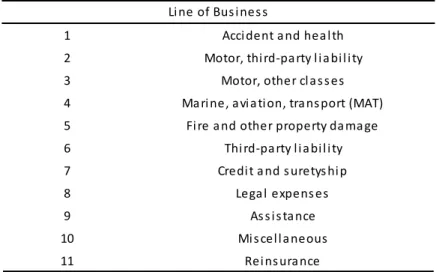
The QIS2 LoB classification is:

CorrNL NLres NLprem NLCAT

NLres 1

NLprem 0.5 1

NLCAT 0 0 1

1 Acci dent a nd hea l th 2 Motor, thi rd-pa rty l i a bi l i ty 3 Motor, other cl a s s es 4 Ma ri ne, a vi a tion, tra ns port (MAT) 5 Fi re a nd other property da ma ge 6 Thi rd-pa rty l i a bi l i ty 7 Credi t a nd s uretys hi p

8 Lega l expens es

9 As s i s tance

10 Mi s cel l a neous

11 Rei ns ura nce

Li ne of Bus i nes s

(37)

36

3.3.1.1 NL PREMIUM RISK

To define the capital requirement for premium risk a factor based approach is used, and it’s:

𝑁𝐿𝑝𝑟= 𝑝(𝜎)𝑃 3.2

Where 𝑃 is the estimate of net earned premium of the overall business in forthcoming year, is the estimate of the standard deviation of the overall combined ratio and is a function of the standard deviation specified as follows:

𝑝(𝑥) =0.99 − 𝜙(𝑁0.99− √𝑙𝑜𝑔(𝑥2+ 1))

0.01 3.3

Where 𝜙 is the cumulative distribution function of the standard normal distribution and

𝑁_0.99 equal to the 99% quantile of the standard normal distribution. In addition the

estimate 𝑃 of the volume of net earned premium for the overall non-life business in the forthcoming year is defined as follows:

𝑃 = ∑ 𝑃_𝑙𝑜𝑏

𝑙𝑜𝑏

3.4

And 𝜎 of the total business is:

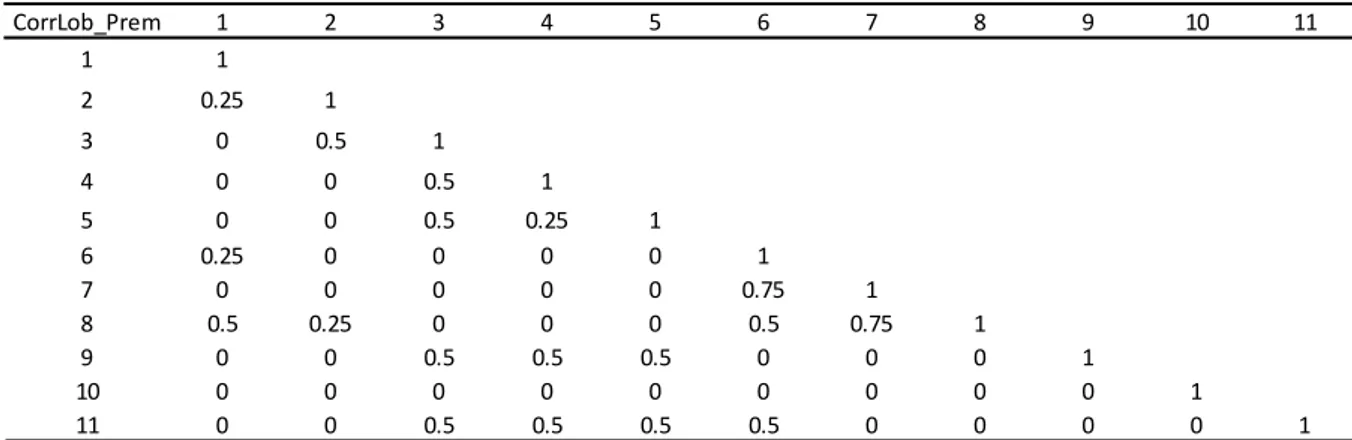
𝜎 = √_𝑃12∑ 𝐶𝑜𝑟𝑟𝐿𝑜𝑏𝑃𝑟𝑟,𝑐∙ 𝑃𝑟∙ 𝑃𝑐∙ 𝜎𝑟∙ 𝜎𝑐

𝑟,𝑐

(38)

37

Table 3: QIS2 Premium Risk LoB correlation.

And 𝜎_𝑟, 𝜎_𝑐 respectively the 𝜎 of 𝑙𝑜𝑏_𝑟 and 𝑙𝑜𝑏_𝑐.

To estimate 𝜎 are available two different approaches:

 “Market-wide approach”;

 “Undertaking-specific approach”.

The market wide approach estimates the standard deviation of the combined ratio in the individual 𝐿𝑜𝐵𝑠 as follows:

𝜎_{𝑀,𝑙𝑜𝑏} = 𝑠𝑓_𝑙𝑜𝑏∙ 𝑓_𝑙𝑜𝑏 3.6

Where 𝑠𝑓𝑙𝑜𝑏 is the size factor defined as follows

𝑠𝑓𝑙𝑜𝑏= { 1 𝑖𝑓 𝑃𝑙𝑜𝑏,𝑔𝑟𝑜𝑠𝑠 > 100𝑚𝑙𝑛 10 √𝑃𝑙𝑜𝑏,𝑔𝑟𝑜𝑠𝑠∙ 10−6 𝑖𝑓 100𝑚𝑙𝑛 > 𝑃_{𝑙𝑜𝑏,𝑔𝑟𝑜𝑠𝑠}≥ 20𝑚𝑙𝑛 10 √20 𝑜𝑡ℎ𝑒𝑟𝑤𝑖𝑠𝑒 3.7

And 𝑓_𝑙𝑜𝑏 is the volatility factor specific for each Line of Business and equal to

CorrLob_Prem 1 2 3 4 5 6 7 8 9 10 11 1 1 2 0.25 1 3 0 0.5 1 4 0 0 0.5 1 5 0 0 0.5 0.25 1 6 0.25 0 0 0 0 1 7 0 0 0 0 0 0.75 1 8 0.5 0.25 0 0 0 0.5 0.75 1 9 0 0 0.5 0.5 0.5 0 0 0 1 10 0 0 0 0 0 0 0 0 0 1 11 0 0 0.5 0.5 0.5 0.5 0 0 0 0 1

(39)

38

The undertaking specific approach estimates the standard deviation of the combined ratio in the individual 𝐿𝑜𝐵𝑠 as follows

𝜎𝑈,𝑙𝑜𝑏 = √𝑐𝑙𝑜𝑏∙ 𝜎𝐶𝑅,𝑙𝑜𝑏2 + (1 − 𝑐𝑙𝑜𝑏) ∙ 𝜎𝑀,𝑙𝑜𝑏2 3.8

Where 𝜎_{𝐶𝑅,𝑙𝑜𝑏}2 _{is the estimate of the standard deviation of the combined ratio in the}

individual 𝑙𝑜𝑏 on the basis of historic combined ratios of the undertaking and 𝑐_𝑙𝑜𝑏 is the

credibility factor for 𝑙𝑜𝑏 defined as

𝑐_𝑙𝑜𝑏= 0.2 ∙ 𝑚𝑎𝑥 ( 0

𝐽_𝑙𝑜𝑏− 10) 3.9

Where 𝐽𝑙𝑜𝑏 is equal to the number of historic combined ratios for each 𝑙𝑜𝑏 (to the

extent available, not more than 15 years). In case of 𝐽𝑙𝑜𝑏> 10 the estimate 𝜎𝐶𝑅,𝑙𝑜𝑏 of

the standard deviation of the combined ratio in the individual 𝑙𝑜𝑏 on the basis of historic combined ratios of the undertaking and is defined as

𝜎𝐶𝑅,𝑙𝑜𝑏= √ 1 (𝐽𝑙𝑜𝑏− 1) ∙ 𝑃𝑙𝑜𝑏∑ 𝑃𝑙𝑜𝑏,𝑦∙ (𝐶𝑅𝑙𝑜𝑏,𝑦− 𝜇𝑙𝑜𝑏) 2 𝑦 3.10 LoB 1 2 3 4 5 6 7 8 9 10 11 flob 0.05 0.125 0.075 0.15 0.10 0.25 0.10 0.15 0.10 0.15 0.15

(40)

39

Where 𝜇_𝑙𝑜𝑏 is the company specific estimate of the expected value of the combined

ratio in the individual 𝑙𝑜𝑏 and equal to

𝜇_𝑙𝑜𝑏=∑ 𝑃𝑦 𝑙𝑜𝑏,𝑦∙ 𝐶𝑅𝑙𝑜𝑏,𝑦

∑ 𝑃𝑦 𝑙𝑜𝑏,𝑦 3.11

3.4 THE STANDARD FORMULA UNDER QIS3

The QIS 3 structure is the following:

QIS3 defines the same risk categories of QIS2 but reviews the structure.

(41)

40

The third quantitative impact study reviewed the non-life underwriting risk module. First of all has been reviewed the aggregation structure unifying the premium and the reserve module and then aggregating the result obtained with the CAT risk capital requirement supposing incorrelation.

Even the LoB classification has been reviewed: Correlation Non-Life

Premium&Reserve Risk

Correlation LoB

Premium by LoB Reserve by LoB

CAT risk

Figure 5: QIS3 aggregation between Premium Risk, Reserve Risk and CAT Risk.

1 Acci dent a nd hea l th-workers compens a tion 2 Acci dent a nd hea l th-hea l th i ns ura nce 3 Acci dent a nd hea l th-others /defa ul t 4 Motor, thi rd-pa rty l i a bi l i ty 5 Motor, other cl a s s es 6 Ma ri ne, a vi a tion, tra ns port (MAT) 7 Fi re a nd other property da ma ge 8 Thi rd-pa rty l i a bi l i ty 9 Credi t a nd s uretys hi p

10 Lega l expens es

11 As s i s tance

12 Mi s cel l a neous non-l i fe i ns ura nce 13 Non-proportiona l rei ns ura nce – property 14 Non-proportiona l rei ns ura nce – ca s ua l ty 15 Non-proportiona l rei ns ura nce – MAT

(42)

41

The capital requirements for Premium & Reserve Risk are determinated multiplying a transformation for the total volume, net of reinsurance, of the reserve amount (only Best Estimate) and the premiums of the following year maintaining an annual growth at least 5%. 𝑁𝐿_𝑝𝑟= 𝑝(𝜎) ∙ 𝑉 3.12 Where 𝑉 = ∑ 𝑉_{𝑝𝑟𝑒𝑚,𝑙𝑜𝑏}+ 𝑉_{𝑟𝑒𝑠,𝑙𝑜𝑏} 𝑙𝑜𝑏 3.13

The function 𝑝(𝜎) is defined as follows

𝑝(𝑥) = 𝑒𝑥𝑝 {−𝜎₂2+ 𝑁_0.995∙ √𝑙𝑜𝑔(𝜎2_{+ 1)} − 1} _3.14

With 𝑁0.995 equal to the 99.5% quantile of the standard normal distribution.

The standard deviation 𝜎 of the combined ratio for the overall non-life insurance portfolio are determinated in two steps:

 in a first step, for each individual line of business standard deviations and

volume measures for both premium risk and reserve risk are determined;

 in a second step, the standard deviations and volume measures for the

premium risk and the reserve risk in the individual 𝑙𝑜𝑏 are aggregated to derive an overall volume measure 𝑉 and an overall standard deviation 𝜎.

(43)

42

LoB 1 2 3 4 5 6 7 8 9 10 11 12 13 14 15

flob 7.5% 3% 5% 10% 10% 12.5% 10% 10% 12.5% 5% 7.5% 12.5% 15% 15% 15% The standard deviation for premium risk in the individual 𝑙𝑜𝑏 is derived as a credibility mix of an undertaking-specific estimate and a market-wide estimate as follows

𝜎𝑝𝑟𝑒𝑚,𝑙𝑜𝑏 = √𝑐𝑙𝑜𝑏∙ 𝜎𝑈,𝑝𝑟𝑒𝑚,𝑙𝑜𝑏2 + (1 − 𝑐𝑙𝑜𝑏) ∙ 𝜎𝑀,𝑝𝑟𝑒𝑚,𝑙𝑜𝑏2 3.15

Where 𝑐_𝑙𝑜𝑏 is the credibility factor for 𝑙𝑜𝑏, 𝜎_{𝑈,𝑝𝑟𝑒𝑚,𝑙𝑜𝑏} is the undertaking-specific

estimate of the standard deviation for premium risk and 𝜎𝑀,𝑝𝑟𝑒𝑚,𝑙𝑜𝑏 is the market-wide

estimate of the standard deviation for premium risk.

The market-wide estimate of the standard deviation for premium risk in the individual 𝑙𝑜𝑏 is determined as follows:

Table 6: QIS3 Premium Risk volatility factors.

And the credibility factor is

𝑐_𝑙𝑜𝑏= {

𝑛_𝑙𝑜𝑏

𝑛_𝑙𝑜𝑏+ 4 𝑖𝑓 𝑛𝑙𝑜𝑏≥ 7

0 𝑜𝑡ℎ𝑒𝑟𝑤𝑖𝑠𝑒

3.16

The undertaking-specific estimate 𝜎_{𝑈,𝑝𝑟𝑒𝑚,𝑙𝑜𝑏} is determined on the basis of the volatility

of historic loss ratios as follows

𝜎_{𝑈,𝑙𝑜𝑏} _{= √} 1

(𝑛𝑙𝑜𝑏− 1) ∙ 𝑉𝑝𝑟𝑒𝑚,𝑙𝑜𝑏∑ 𝑃𝑙𝑜𝑏,𝑦∙ (𝐿𝑅𝑙𝑜𝑏,𝑦− 𝜇𝑙𝑜𝑏)

2 𝑦

(44)

43

Where 𝜇_𝑙𝑜𝑏 is the company-specific estimate of the expected value of the Loss Ratio in

the individual 𝑙𝑜𝑏 and it’s defined as the premium-weighted average of historic Loss Ratios

𝜇𝑙𝑜𝑏=

∑ 𝑃𝑦 𝑙𝑜𝑏,𝑦∙ 𝐿𝑅𝑙𝑜𝑏,𝑦

∑ 𝑃_𝑦 _{𝑙𝑜𝑏,𝑦} 3.18

The standard deviations for reserve risk in the individual 𝑙𝑜𝑏 are the following

The overall volume measure 𝑉 is determined as follows

𝑉 = ∑ 𝑉_{𝑝𝑟𝑒𝑚,𝑙𝑜𝑏}+ 𝑉_{𝑟𝑒𝑠,𝑙𝑜𝑏}

𝑙𝑜𝑏

3.19

The overall standard deviation 𝜎 is determined as follows

𝜎 = √_𝑉12∑ 𝐶𝑜𝑟𝑟𝐿𝑜𝑏𝑟,𝑐∙ 𝑉𝑟∙ 𝑉𝑐∙ 𝑎𝑟∙ 𝑎𝑐

𝑟,𝑐

3.20

Where 𝑟, 𝑐 are indices of the form (𝑝𝑟𝑒𝑚, 𝑙𝑜𝑏) or (𝑟𝑒𝑠, 𝑙𝑜𝑏), 𝑉𝑟 and 𝑉𝑐 are volume

measures for the individual line of business, the factors 𝑎𝑟 and 𝑎𝑐 are defined as follows

LoB 1 2 3 4 5 6 7 8 9 10 11 12 13 14 15

flob 15% 7.5% 15% 12.5% 7.5% 15% 10% 15% 10% 10% 10% 15% 15% 20% 20%

(45)

44

𝑎𝑟 = {

𝜎_{𝑝𝑟𝑒𝑚,𝑙𝑜𝑏} 𝑖𝑓 𝑟 = (𝑝𝑟𝑒𝑚, 𝑙𝑜𝑏)

𝜎_{𝑟𝑒𝑠,𝑙𝑜𝑏} 𝑖𝑓 𝑟 = (𝑟𝑒𝑠, 𝑙𝑜𝑏) 3.21

And 𝐶𝑜𝑟𝑟𝐿𝑜𝑏𝑟,𝑐_{is the correlation matrix defined as}

𝐶𝑜𝑟𝑟𝐿𝑜𝑏𝑟,𝑐 _{= [} 𝐶𝑜𝑟𝑟𝐿𝑜𝑏𝑝𝑟 0.5 ∙ 𝐶𝑜𝑟𝑟𝐿𝑜𝑏𝑝𝑟

0.5 ∙ 𝐶𝑜𝑟𝑟𝐿𝑜𝑏_𝑝𝑟 𝐶𝑜𝑟𝑟𝐿𝑜𝑏_𝑝𝑟 ] 3.22

With 𝐶𝑜𝑟𝑟𝐿𝑜𝑏𝑝𝑟

3.5 THE STANDARD FORMULA UNDER QIS4

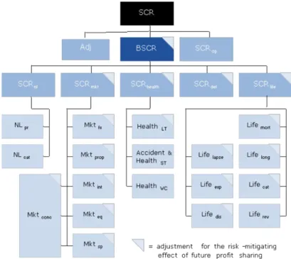
The QIS3 structure is utilized even in QIS4. The total capital requirement is determined adding to the operational risk capital requirement, assuming full correlation with all the other risks but, differently from QIS3, are subtracted two adjustments for future discretionary benefit and for the deferred taxes:

CorrLob_Pr 1 2 3 4 5 6 7 8 9 10 11 12 13 14 15 1 1 2 0.5 0.5 3 0.5 0.5 1 4 0.25 0.25 0.25 1 5 0.25 0.25 0.25 0.5 1 6 0.25 0.25 0.25 0.5 0.25 1 7 0.25 0.25 0.25 0.25 0.25 0.25 1 8 0.5 0.25 0.25 0.5 0.25 0.25 0.25 1 9 0.25 0.25 0.25 0.25 0.25 0.25 0.25 0.5 1 10 0.5 0.25 0.5 0.5 0.5 0.25 0.25 0.5 0.5 1 11 0.25 0.25 0.25 0.25 0.5 0.5 0.5 0.25 0.25 0.25 1 12 0.5 0.5 0.5 0.5 0.5 0.5 0.5 0.5 0.5 0.5 0.5 1 13 0.25 0.25 0.25 0.25 0.25 0.25 0.5 0.25 0.25 0.25 0.5 0.25 1 14 0.25 0.25 0.25 0.25 0.25 0.25 0.25 0.5 0.5 0.5 0.25 0.25 0.25 1 15 0.25 0.25 0.25 0.25 0.25 0.5 0.5 0.25 0.25 0.25 0.25 0.5 0.25 0.25 1

(46)

45

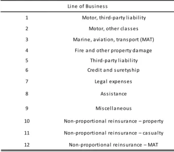
The 𝑙𝑜𝑏 classification has been reviewed in QIS4:

Figure 6: QIS4 SCR Structure.

1 Motor, thi rd-pa rty l i a bi l i ty 2 Motor, other cl a s s es 3 Ma ri ne, a vi a ti on, tra ns port (MAT) 4 Fi re a nd other property da ma ge 5 Thi rd-pa rty l i a bi l i ty 6 Credi t a nd s uretys hi p

7 Lega l expens es

8 As s i s ta nce

10 Non-proporti ona l rei ns ura nce – property 11 Non-proporti ona l rei ns ura nce – ca s ua l ty 12 Non-proporti ona l rei ns ura nce – MAT

(47)

46

For the non-life module, the QIS 4 maintains the same standard of QIS3 with some modifications: 𝑁𝐿_𝑝𝑟= 𝑝(𝜎) ∙ 𝑉 3.23 𝑉 = ∑ 𝑉_𝑙𝑜𝑏 𝑙𝑜𝑏 3.24 𝑉_𝑙𝑜𝑏= (𝑉𝑝𝑟𝑒𝑚,𝑙𝑜𝑏+ 𝑉𝑟𝑒𝑠,𝑙𝑜𝑏) ∙ (0.75 + 0.25 ∙ 𝐷𝐼𝑉𝑝𝑟,𝑙𝑜𝑏) 3.25 𝐷𝐼𝑉_{𝑝𝑟,𝑙𝑜𝑏}= ∑ (𝑉𝑝𝑟𝑒𝑚,𝑗,𝑙𝑜𝑏+ 𝑉𝑟𝑒𝑠,𝑗,𝑙𝑜𝑏) 2 𝑗 {∑ (𝑉𝑗 𝑝𝑟𝑒𝑚,𝑗,𝑙𝑜𝑏+ 𝑉𝑟𝑒𝑠,𝑗,𝑙𝑜𝑏)}2 3.26

That meant it’s introduced a geographical diversification.

The new market-wide estimate of the standard deviation for premium risk in the individual 𝑙𝑜𝑏 are

The maximum value of for the determination of is fixed according to the line of business in the following table:

Table 10: QIS4 Premium Risk volatility factors.

LoB 1 2 3 4 5 6 7 8 9 10 11 12

(48)

47

LoB 1 2 3 4 5 6 7 8 9 10 11 12

σ(res,lob) 12% 7% 10% 10% 15% 15% 10% 10% 10% 15% 20% 20%

Table 11: QIS4 maximum number of 𝒏𝒍𝒐𝒃.

The new values of the standard deviation for reserve risk in the individual 𝑙𝑜𝑏 are:

Table 12: QIS4 Reserve Risk volatility factors.

In QIS4 after having derived 𝜎𝑝𝑟𝑒𝑚,𝑙𝑜𝑏 and 𝜎𝑟𝑒𝑠,𝑙𝑜𝑏 the standard deviation for premium

and reserve risk in the individual 𝑙𝑜𝑏 is defined by aggregating the standard deviations for both subrisks under the assumption of a correlation coefficient of 𝛼 = 0.5

𝜎𝑙𝑜𝑏 =√(𝜎𝑝𝑟𝑒𝑚,𝑙𝑜𝑏∙ 𝑉𝑝𝑟𝑒𝑚,𝑙𝑜𝑏) 2 + (𝜎𝑟𝑒𝑠,𝑙𝑜𝑏∙ 𝑉𝑟𝑒𝑠,𝑙𝑜𝑏) 2 + 2 ∙ 𝛼 ∙ (𝜎𝑝𝑟𝑒𝑚,𝑙𝑜𝑏∙ 𝑉𝑝𝑟𝑒𝑚,𝑙𝑜𝑏) ∙ (𝜎𝑟𝑒𝑠,𝑙𝑜𝑏∙ 𝑉𝑟𝑒𝑠,𝑙𝑜𝑏) 𝑉𝑝𝑟𝑒𝑚,𝑙𝑜𝑏+ 𝑉𝑟𝑒𝑠,𝑙𝑜𝑏 3.27

The credibility factor 𝑐_𝑙𝑜𝑏 are defined as

LoB Ma xi mum nlob

2, 4, 7, 8, 10 5 3, 9, 12 10 1, 5, 6, 11 15

Maximum value of nlob 1 2 3 4 5 6 7 8 9 10 11 12 13 14 15 15 0 0 0 0 0 0 0.64 0.67 0.69 0.71 0.73 0.75 0.76 0.78 0.79 10 0 0 0 0 0.64 0.69 0.72 0.74 0.76 0.79 - - - - -

5 0 0 0.64 0.72 0.79 - - - - - - - - -

-Number of historical years of data available (excluding the first 3 years after the line of business was first written)

(49)

48

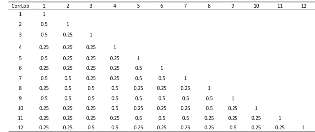
Finally the new correlation matrix is:

3.6 THE STANDARD FORMULA UNDER QIS5

The QIS5 structure is:

CorrLob 1 2 3 4 5 6 7 8 9 10 11 12 1 1 2 0.5 1 3 0.5 0.25 1 4 0.25 0.25 0.25 1 5 0.5 0.25 0.25 0.25 1 6 0.25 0.25 0.25 0.25 0.5 1 7 0.5 0.5 0.25 0.25 0.5 0.5 1 8 0.25 0.5 0.5 0.5 0.25 0.25 0.25 1 9 0.5 0.5 0.5 0.5 0.5 0.5 0.5 0.5 1 10 0.25 0.25 0.25 0.5 0.25 0.25 0.25 0.5 0.25 1 11 0.25 0.25 0.25 0.25 0.5 0.5 0.5 0.25 0.25 0.25 1 12 0.25 0.25 0.5 0.5 0.25 0.25 0.25 0.25 0.5 0.25 0.25 1

Figure 7: QIS5 SCR Structure. Table 14: QIS4 Premium Risk LoB correlation.

(50)

49

The capital requirement for non-life underwriting risk is derived by combining the capital requirements for the non-life sub-risks using a correlation matrix as follows

𝑆𝐶𝑅_𝑛𝑙𝑄𝐼𝑆5_{= √∑ 𝐶𝑜𝑟𝑟}𝑟⋅𝑐_𝑁𝐿

𝑟𝑁𝐿𝑐 𝑟⋅𝑐

3.28

Where 𝐶𝑜𝑟𝑟𝑟⋅𝑐_{is set equal to}

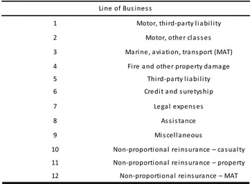
The 𝑙𝑜𝑏 classifications is not reviewed in QIS5

CorrNL NLres NLprem NLCAT

NLres 1

NLprem 0 1

NLCAT 0 0.25 1

1 Motor, thi rd-pa rty l i a bi l i ty 2 Motor, other cl a s s es 3 Ma ri ne, a vi a tion, tra ns port (MAT) 4 Fi re a nd other property da ma ge 5 Thi rd-pa rty l i a bi l i ty 6 Credi t a nd s uretys hi p 7 Lega l expens es

8 As s i s tance

10 Non-proportiona l rei ns ura nce – property 11 Non-proportiona l rei ns ura nce – ca s ua l ty 12 Non-proportiona l rei ns ura nce – MAT

Table 16: QIS5 LoB classification.

(51)

50

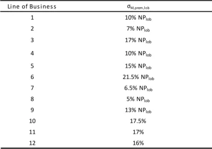
The QIS5 standard formula is the same of QIS4 but introduces some modifications. The market-wide estimates of the net standard deviation for premium risk for each line of business are:

Where the adjustment factor for non-proportional reinsurance of a line of business allows undertakings to take into account the risk-mitigating effect of particular per risk excess of loss reinsurance.

The volatility factors for the reserve risk are:

LoB 1 2 3 4 5 6 7 8 9 10 11 12

σ_(res,lob) 9.5% 10% 14% 11% 11% 19% 9% 11% 15% 20% 20% 20%

Li ne of Bus i nes s σM,prem,lob

1 10% NPlob 2 7% NPlob 3 17% NPlob 4 10% NPlob 5 15% NPlob 6 21.5% NPlob 7 6.5% NPlob 8 5% NPlob 9 13% NPlob 10 17.5% 11 17% 12 16%

Table 18: QIS5 Reserve Risk volatility factors. Table 17: QIS5 Premium Risk volatility factors.

(52)

51 3.7 THE STANDARD FORMULA UNDER LONG TERM GUARANTEE

ASSESMENT

The LTG structure is

The capital requirement for non-life underwriting risk is derived by combining the capital requirements for the non-life sub-risks using a correlation matrix as follows

(53)

52

𝑆𝐶𝑅_𝑛𝑙𝐿𝑇𝐺 _{= √∑ 𝐶𝑜𝑟𝑟}𝑟⋅𝑐_𝑁𝐿

𝑟𝑁𝐿𝑐 𝑟⋅𝑐

3.29

Where 𝐶𝑜𝑟𝑟𝑟⋅𝑐_{is set equal to}

Table 19: LTGA correlation matrix between reserve&premium risk, lapse risk and CAT risk

The capital requirement for the combined premium and reserve risk is determined as follows

𝑁𝐿𝑝𝑟= 3 ∙ 𝜎 ∙ 𝑉 3.30

𝑉 is the volume measure and 𝜎 is the standard deviation of the overall non-life insurance portfolio and are determined in two steps:

 for each 𝑙𝑜𝑏 the standard deviations and volume measures for both premium

and reserve risk are determined;

 the standard deviations and volume measures for the premium risk and the

reserve risk in the individual 𝑙𝑜𝑏 are aggregated to derive an overall volume measure 𝑉 and a combined standard deviation 𝜎.

The premium and reserve risk sub-module is based on the following segmentation

CorrNL NLpr NLlapse NLCAT

NLpr 1

NLlapse 0 1

A pricing technique to calculate the solvency capital requirement for non-life premium risk

0