I would like to begin by expressing my thanks to Prof. Annamaria Canino for her encouragement and support during all these years.
I would also to thank Prof. Ireneo Peral for his valuable advise. He always shows interest in my work and his discussions have given me new ideas.
A special thanks goes to Prof. Jesus Azorero and to Prof. Andrea Malchiodi. I feel privileged for the opportunity to work with them and I am very grateful for their valuable help.
I am also thankful to Raffaella Servadei for being close in this period and for her deeply friendship.
I would like to thank warmly Dino Sciunzi for many fruitful conversa-tions.
Infine un ringraziamento speciale va alla mia famiglia che mi `e vicina e mi sostiene sempre.
Acknowledgments i
Introduction ix
1 Preliminaries 1
1.1 A uniqueness result . . . 1
1.2 Perturbation methods . . . 2
1.2.1 Critical points for the perturbed functional Iε . . . 3
1.2.2 The singular perturbation case . . . 4
1.2.3 A technical lemma for the Neumann case . . . 4
1.2.4 Some estimates for the Neumann problem . . . 5
1.3 A classical variational theorem . . . 5
1.4 The Perron method . . . 7
1.5 A monotonicity result . . . 7
1.6 Some useful results about the least-energy solutions to a semi-linear perturbed Neumann problem . . . 8
1.7 The Lax-Milgram lemma . . . 9
1.8 Notations . . . 10
2 Concentration of solutions and Perturbation Methods 11 2.1 The mixed perturbed problem . . . 12
2.1.1 Perturbation in critical point theory . . . 12
2.1.2 Approximate solutions for (Pε) with Neumann condi-tions . . . 15
2.2 Approximate solutions to (Pε) . . . 21
2.2.1 Asymptotic analysis of (2.31) . . . 23
2.2.2 Definition of the approximate solutions and study of their accuracy . . . 34
2.3 Proof of Theorem 2.0.1 . . . 42
2.3.1 Energy expansions for the approximate solutions ˆzε,Q 42 2.3.2 Finite-dimensional reduction and study of the con-strained functional . . . 47
vi CONTENTS
3 Asymptotics of least energy solutions 53
3.1 The least energy solution . . . 56
3.2 Straightening the boundary . . . 59
3.2.1 Convergence of scaled function . . . 60
3.3 Analysis of the limit points Pε . . . 70
3.4 Location of the least energy solution . . . 81
4 The shape of the least-energy solution 91 4.1 The Mountain Pass geometry . . . 93
4.1.1 The Palais-Smale (P S)c condition . . . 95
4.2 The steepest descent direction . . . 96
4.3 Solution of problem (Pv) . . . 98
4.3.1 Numerical approximation . . . 99
4.4 The numerical algorithm . . . 102
4.4.1 Step 1 of the algorithm . . . 102
4.4.2 Step 2 of the algorithm . . . 102
4.4.3 Step 3 of the algorithm . . . 103
1.1 The Mountain Pass Geometry. . . 6
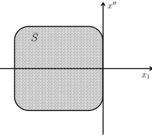
2.1 The domain ˜S. . . 22
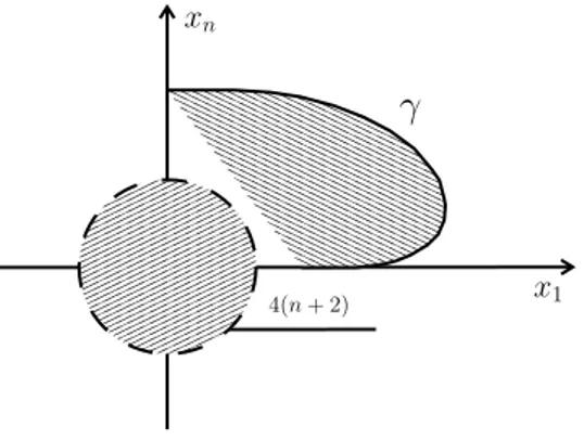
2.2 The curve γ in the (x1, xn) plane. . . 23
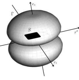
2.3 The domain ˆΓ. . . 24
3.1 Phase plane. . . 55
3.2 Flattening & Scaling . . . 61
3.3 Moving plane . . . 73
3.4 The compact K . . . 76
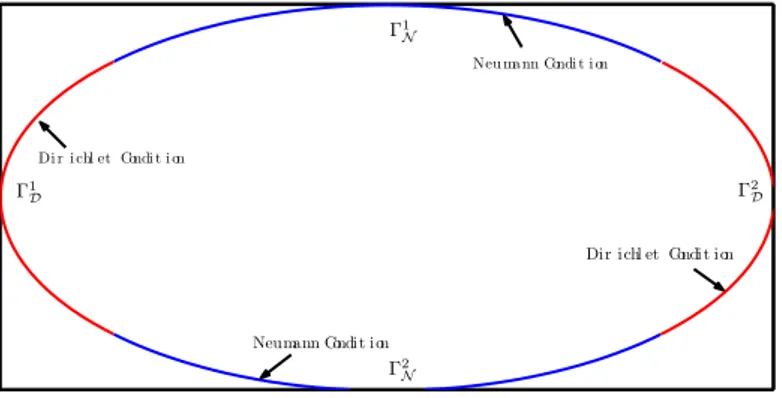
4.1 The Elliptical Domain Ω. . . 91
4.2 Subdivision of the domain Ω into triangles. . . 101
4.3 Three-dimensional view with ε = 0.7. . . 104
4.4 Two-dimensional view with ε = 0.7. . . 105
4.5 Three-dimensional view with ε = 0.4. . . 106
4.6 Two-dimensional view with ε = 0.4. . . 106
4.7 Three-dimensional view with ε = 0.2. . . 107
4.8 Two-dimensional view with ε = 0.2. . . 107
4.9 Three-dimensional view with ε = 0.1. . . 108
The theory of Partial Differential Equations, and in particular the
Nonlin-ear Equations, is an important tool to describe real models. In fact, many
problems coming from science and engineering are described by nonlinear differential equations, which can be notoriously difficult to solve. This is also the case of the equations we study in this thesis.
The aim of this work is to analyze some elliptic equations that are per-turbative in nature. We will examine our problem using two tools:
(i) perturbative methods; (ii) variational methods.
In particular, in this thesis, we are interested in the following perturbed mixed problem −ε2∆u + u = up in Ω; ∂u ∂ν = 0 on ∂NΩ; u = 0 on ∂DΩ; u > 0 in Ω, ( ˜Pε)
where Ω is a smooth bounded subset of Rn, p ∈ ³1,n+2 n−2
´
, ε > 0 is a small parameter, and ∂NΩ, ∂DΩ are two subsets of the boundary of Ω such
that the union of their closures coincides with the whole ∂Ω. This type of perturbative equations, with Neumann conditions or Dirichlet conditions, were been studied in literature by many authors, see for example [2], [21], [49], [50] and [51].
Nevertheless these problems, with mixed conditions, appear in several situations. Generally the Dirichlet condition is equivalent to impose some
state on the physical parameter represented by u, while the Neumann
condi-tions give a meaning at the flux parameter crossing ∂NΩ. Here below there are some common physical applications of such problems:
• Population dynamics. Assume that a species lives in a bounded region
Ω such that the boundary has two parts, ∂NΩ and ∂DΩ, where the
first one is an obstacle that blocks the pass across, while the second one is a killing zone for the population.
x INTRODUCTION
• Nonlinear heat conduction. In this case ( ˜Pε) models the heat (for
small conductivity) in the presence of a nonlinear source in the interior of the domain, with combined isothermal and isolated regions at the boundary.
• Reaction diffusion with semi-permeable boundary. In this framework
we have that the meaning of the Neumann part, ∂NΩ, is an obstacle
to the flux of the matter, while the Dirichlet part, ∂DΩ, stands for a semipermeable region that allows the outwards transit of the matter produced in the interior of the cell Ω by the reaction represented by a general nonlinearity f (u).
Partial differential equations, as the one in ( ˜Pε), also appear in the study
of reaction-diffusion systems. For single equations with Neumann boundary conditions it is known that when Ω is convex the only stable solutions are constants, see [12] and [45]. On the other hand, as noticed in [55], reaction-diffusion systems with different diffusivities might lead to non-homogeneous stable steady states. A well-know example is the following one (Gierer-Meinhardt) Ut= d1∆U − U +U p Vq in Ω × (0, +∞), Vt= d2∆V − V + U r Vs in Ω × (0, +∞), ∂U ∂ν = ∂V∂ν = 0 on ∂Ω × (0, +∞), (GM )
introduced in [28] to describe some biological experiment. The functions
U and V represent the densities of some chemical substances, the numbers p, q, r, s are non-negative and such that 0 < p−1q < r
s+1, and it is assumed
that the diffusivities d1 and d2 satisfy d1 ¿ 1 ¿ d2. In the stationary case
of (GM ), as explained in [48], when d2 → +∞ the function V is close to
a constant (being nearly harmonic and with zero normal derivative at the boundary), and therefore the equation satisfied by U resembles the first one in ( ˜Pε). Clearly a similar reduction procedure could be used when mixed
boundary conditions are imposed.
Let us now describe some results which concern singularly perturbed problems, with Neumann or Dirichlet boundary conditions, well studied by different authors (see, for example, [2], [20], [48], [49], [50] and [51]), and
specifically (Nε) −ε2∆u + u = up in Ω; ∂u ∂ν = 0 on ∂NΩ; u > 0 in Ω, (Dε) −ε2∆u + u = up in Ω; u = 0 on ∂DΩ; u > 0 in Ω.
These problems arise also as limits of reaction-diffusion systems different from (GM ) (with chemotaxis for example, as shown in [48]).
Another motivation comes from the Nonlinear Schr¨odinger equation (in short NLS)
i~∂ψ ∂t = −~
2∆ψ + V (x)ψ − |ψ|p−1ψ in Rn,
where ψ is a complex-valued function (the wave function), V is a potential and p is an exponent greater than 1. NLS of this sort are used, for example, in Plasma Physics, but also arise in Nonlinear Optics. Indeed, if one looks for standing waves, namely solutions of the form ψ(x, t) = e−iωt~ u(x), for some real function u, then the latter will satisfy
−ε2∆u + V (x)u = up in Rn,
where we have set ε = ~ and we absorbed the constant ω into the potential
V . Therefore, up to the potential, we still obtain the equation in (Nε) or
(Dε): about this subject we refer the reader to the (still incomplete) list of
papers [1], [2], [6], [24] and to the bibliographies therein.
The typical concentration behavior of solutions uεto the above two
prob-lems is via a scaling of the variables in the form uε(x) ∼ U
³
x−Q ε
´
, where Q is some point of Ω, and U , see Section 1.1, is a solution of
−∆U + U = Up in Rn (or in Rn+= {(x1, . . . , xn) ∈ Rn: xn> 0}), (1)
the domain depending on whether Q lies in the interior of Ω or at the boundary; in the latter case Neumann conditions are imposed. When p <
n+2
n−2 (and indeed only if this inequality is satisfied), such problem (1) admits
positive radial solutions which decay to zero at infinity, see Proposition 1.1.1. Solutions of ( ˜Pε) which inherit this profile are called spike layers, since
they are highly concentrated near some point of Ω. There is an extensive literature regarding this type of solutions, beginning from the papers [38], [49] and [50]. Indeed their structure is very rich, and we refer for example to the (far from complete) list of references [17], [20], [31], [32], [33], [34], [36], [37], [56] and [57].
xii INTRODUCTION
Spike layers solving (Nε) and sitting on the boundary of Ω are peaked
near critical points of the mean curvature of ∂Ω. To see this one can exploit the variational structure of the problem, whose Euler functional is
˜ Iε,N(u) = 12 Z Ω ¡ ε2|∇u|2+ u2¢− 1 p + 1 Z Ω |u|p+1; u ∈ H1(Ω). (2) Plugging into ˜Iε,N a function of the form UQ,ε(x) = U¡1
ε(x − Q)
¢ with
Q ∈ ∂Ω one sees that
˜
Iε,N(UQ,ε) = ˜C0εn− ˜C1εn+1H(Q) + o(εn+1),
where ˜C0, ˜C1 are positive constants depending only on n and p and H
de-notes the mean curvature.
This expansion can be obtained using the radial symmetry of U and parameterizing ∂Ω as a normal graph near Q. From the above formula we see that, the bigger is the mean curvature the lower is the energy of this function: roughly speaking, boundary spike layers would tend to move along the gradient of H in order to minimize their energy. Indeed in [49], [50] it was shown that Mountain Pass solutions to (Nε) (ground states) have only
one local maximum over Ω and it concentrates at ∂Ω near global maxima of the mean curvature.
Concerning instead (Dε), spike layers with minimal energy concentrate at the interior of the domain, at points which maximize the distance from the boundary, see [51]. The intuitive reason for this is that, if Q is in the interior of Ω and if we want to adapt a function like U¡1
ε(x − Q)
¢ to the Dirichlet conditions, the adjustment needs an energy which increases as Q becomes closer and closer to ∂Ω. Following the above heuristic argument, we could say that spike layers are repelled from the regions where Dirichlet conditions are imposed.
In this thesis, we are interested in finding boundary spike layers for the mixed problem ( ˜Pε). First, we apply a perturbative approach: the idea
is to obtain two compensating effects from the Neumann and the Dirichlet conditions. More precisely, calling IΩthe intersection of the closures of ∂DΩ and ∂NΩ, and assuming that the gradient of H at IΩ points toward ∂DΩ,
a spike layer centered on ∂NΩ will be pushed toward IΩ by ∇H and will be
repelled from IΩ by the Dirichlet condition.
Our main result will show that there exists a solution uεto the problem
( ˜Pε) concentrating at the interface IΩ. The general strategy used relies
on a finite-dimensional reduction, which is conceptually rather simple and nowadays well understood, see Chapter 1 or, for example, the book [2]. One finds first a manifold Z of approximate solutions to the given problem, which in our case are of the form U¡1
ε(x − Q)
¢
, and solve the equation up to a vector (in the Hilbert space) parallel to the tangent plane of this manifold.
In this way, see Proposition 2.1.3, one generates a new manifold ˜Z close to Z
which represents a natural constraint for the Euler functional of ( ˜Pε), which
is ˜ Iε(u) = 12 Z Ω ε2|∇u|2+ u2− 1 p + 1 Z Ω |u|p+1; u ∈ HD1(Ω). (3) Here H1
D(Ω) stands for the space of functions in H1(Ω) which have zero
trace on ∂DΩ, and by natural constraint we mean a set for which constrained
critical points of ˜Iε are true critical points.
The main difficulty however is to have a good control of ˜Iε|Z˜, which
is done improving the accuracy of the functions in the original manifold
Z: in fact, the better is the accuracy of these functions, the closer is ˜Z to Z, so the main term in the constrained functional will be given by ˜Iε|Z, see Proposition 2.2.12 and Lemma 2.3.5 below. To find sufficiently good approximate solutions we start with those constructed in literature for the Neumann problem (Nε) (see Chapter 2, Section 2.1.2) which reveal the role of the boundary mean curvature, as in the expansion after (2). However these functions are not zero on ∂DΩ, and if one tries naively to annihilate
them using cut-off functions, the corresponding error turns out to be too large. A method which revealed itself to be useful for (Dε) is to consider the projection operator in H1(Ω), which consists in associating to some function
in this space its closest element in H1
D(Ω). In some previous works, see for
example [37] and [58], the asymptotic behavior of this projection has been studied in detail when the limit concentration point lies in the interior of Ω, using (see Chapter 1, equations (1.3) and (1.4)) the well known limit behavior of the solution U to (1),
lim
r→+∞e rrn−1
2 U (r) = αn,p,
where the positive constant αn,p depends only on n and p, together with
lim r→+∞ U0(r) U (r) = −1; r→+∞lim U00(r) U (r) = 1.
In our case instead, apart from having mixed conditions, the maxima of the spike-layers tend to the interface IΩ, so, to better understand the projection, we need to work at a scale d ' ε| log ε|, the order of the distance of the peak from IΩ. At this scale the boundary of the domain looks nearly flat, so
in this step we replace Ω with a non smooth domain ˆΓD ⊆ Rn such that
part of ∂ ˆΓD looks like a cut of dimension n − 1. We choose ˆΓD to be
even with respect to the coordinate xn and we study H1 projections here
(with Dirichlet conditions) which are also even in xn: as a consequence we will find functions which have zero xn-derivative on {xn= 0} \ ∂ ˆΓD, which
mimics the Neumann boundary condition on ∂NΩ. After analyzing carefully
the projection we define a family of suitable approximate solutions to ( ˜Pε),
xiv INTRODUCTION
We can finally apply the above mentioned perturbation method to reduce the problem to a finite dimensional one, and study the functional constrained on ˜Z. If zε
Q denotes (roughly speaking) an approximate solution peaked at Q, with dist(Q, IΩ) = dε, then its energy turns out to be the following
˜ Iε(zQε) = εn ³ ˜ C0− ˜C1εH(Q) + e−2dεε(1+o(1))+ O(ε2) ´ .
The first two terms in this formula are as in the expansion after (2) for (Nε),
while the third one represents a sort of potential energy which decreases with the distance of Q from the interface, consistently with the repulsive effect which was described before for (Dε). From the latter formula it follows
that, if dε remains constant, then we recover the expansion corresponding
to the Neumann problem. On the other hand even if dε → 0, that is when
the concentration points converge to the interface, one can check that the energy has a critical point when H|IΩ is stationary, provided ∇H points toward ∂DΩ, and dε ' ε| log ε|.
Next in the thesis, via variational methods, we analyze also the asymp-totic profile of the least energy solutions to the problem ( ˜Pε) under generic
assumptions on the domain and on the interface.
First we show that Mountain Pass solutions are in fact least energy solutions. Then we prove that, given a family of least energy solutions {uε},
their points of maximum must lie on the boundary of the domain Ω, as in the Neumann case.
We also analyze the rate of convergence to specify better the location of maximum limit points Pε of the least energy solutions as ε → 0: we
show that the concentration point cannot belong to the interior of Dirichlet boundary part. To obtain these results, we use the moving plane method proving also an important Liouville type result, see Lemma 3.3.2. Next, we characterize the shape of least energy solutions showing that, also in the Mixed case, such solutions can be approximated by the ground state solution U to the problem (1). This fact follows from other results proved in the thesis; in particular we have that, after a scaling, the maximum Pε
(indeed unique, see Theorem 3.3.9) of the solutions uε is always bounded away from the interface IΩ as ε → 0.
Moreover, we prove that, as for (Nε), the least energy solutions
concen-trate at boundary points in the closure of ∂NΩ where the mean curvature is maximal. When this constrained maximum is attained on the interface (and if ∇H here is non zero), we will be able to show that the Mountain Pass solution has precisely the behavior found in Theorem 2.0.1 by perturbative methods.
In the last part of the thesis we consider the least energy solutions to the problem ( ˜Pε) and, via numerical algorithm, we construct their shape and
we present the related results.
We use a numerical method which allows us to find solutions of Mountain Pass type. Such a method was introduced by Y.S.Choi and P.J.McKenna in [14] for some elliptic equations in square domains. Instead, we consider a particular case of ( ˜Pε), choosing p = 3 and n = 2, namely
−ε2∆u + u = u3 in Ω; ∂u ∂ν = 0 on ∂NΩ; u = 0 on ∂DΩ; u > 0 in Ω, ( e˜Pε)
where Ω is a bounded domain of R2.
Such a problem is perturbative one with mixed boundary conditions that are numerically difficult to deal with.
We define problem ( e˜Pε) in a bounded elliptical domain of R2 in order to
have a non constant mean curvature H to find Mountain Pass type solutions concentrating at the interface IΩ. Then, we need to mesh Ω in order to
describe and define the discrete differential problem associated to ( e˜Pε).
We want to point out that, from the numerical point of view, curved boundary domains, such as the elliptical ones, are generally more difficult to treat than the square ones.
All the algorithm, used to get the shape of least energy (Mountain Pass type) solutions of ( e˜Pε), was implemented with a MATLAB code.
This thesis is organized as follows.
In Chapter 1 we will recall some tools of nonlinear analysis which are em-ployed in the rest of the thesis. For a better understanding, we will examine the perturbative approach in critical point theory, in particular referring to the singularly perturbed Neumann problem. Then we will recall some def-initions and some theorems about critical point theory. We also will give some notations.
In Chapter 2 we will deal with the existence results and the asymptotic behavior of some solutions to the singularly perturbed problem ( ˜Pε) with
mixed Dirichlet and Neumann conditions by using perturbative methods. These results were been obtained in [25].
In Chapter 3 we will analyze the location and the shape of the least energy
solutions to the problem ( ˜Pε), when the singular perturbation parameter tends to zero, via variational methods. The results presented in this chapter were been achieved in [26].
In Chapter 4 we will present some results about the construction of the shape of the least energy solutions to the problem ( ˜Pε) via numerical
Chapter 1
Preliminaries
In this chapter we will recall the fundamental tools and definitions which will be employed in this thesis. We also will give some notations.
1.1
A uniqueness result
Let us consider the following problem
−∆U + U = Up in Rn. (1.1)
Corresponding to (1.1) we define an energy of a function u ∈ H1(Rn): I(u) := 1 2 Z Rn (| ∇u|2+ u2) − 1 p + 1 Z Rn |u|p+1 (1.2) Proposition 1.1.1 If p ∈ ³ 1,n+2n−2 ´
problem (1.1) admits a solution U sat-isfying
(i) U ∈ C2(Rn) ∩ H1(Rn) and U > 0 in Rn;
(ii) U is spherically symmetric: U (x) = U (r) with r = |x| and dU
dr < 0 for r > 0;
(iii) U and its first derivatives decay exponentially at infinity, i.e., there exists a positive constant αn,p depending only on n and p such that
lim r→+∞e rrn−12 U (r) = α n,p, (1.3) and lim r→+∞ U0(r) U (r) = −1; r→+∞lim U00(r) U (r) = 1; (1.4)
(iv) for any non-negative solution u ∈ C2(Rn) ∩ H1(Rn) to (1.1),
0 < I(U ) ≤ I(u)
holds unless u ≡ 0.
Remark 1.1.2 M.K.Kwong [35] showed that radial solutions to (1.1) are
unique when p ∈ ³ 1,n+2 n−2 ´ .
Remark 1.1.3 Sometimes, through the thesis, we will call ground state,
the solution given by Proposition 1.1.1 and Remark 1.1.2 .
1.2
Perturbation methods
In this section, we want to give just a very short outline to the perturbation methods to better understand the basic ideas used in the sequel of the thesis. However for more details about the perturbation methods we refer strongly to the book [2].
There are several elliptic problems on Rn which are perturbative in
na-ture. For these perturbation problems a specific approach, that takes advan-tage of such a perturbative setting, seems the most appropriate. Actually, it turns out that such framework can be used to handle a large variety of equa-tions, different in nature. These problems can be studied using a common abstract setting.
Let H be a Hilbert space. We look for critical point of a sufficiently smooth functional Iε : H → R depending on a small perturbative parameter ε ∈ R, that is solutions of equation
Iε0(u) = 0, u ∈ H. (1.5)
Generally, in the perturbative methods, one arranges the functional Iε
associated to the differential problem in a functional like
Iε(u) = I0(u) + εG(u),
where I0 is called unperturbed functional and G is a perturbation. On
the Perturbation theory one supposes that I0 possesses non-isolated crit-ical points which form a manifold Z referred to as a critcrit-ical manifold, that is:
Z = {z ∈ H : I00(z) = 0}. (1.6) Let TzZ be the tangent space to Z at z, we denote the orthogonal
comple-ment to TzZ as
W = (TzZ)⊥. (1.7)
In this case, finding solutions of I0
ε(u) = 0 becomes a kind of bifurcation
1.2 Perturbation methods 3
Z ⊂ R × H is the set of the trivial solutions. One looks for conditions
on the perturbation G that generate non-trivial solutions, namely a pair (ε, u) ∈ R × H, with ε 6= 0, such that I0
ε(u) = 0. In this context, in order to
solve equation (1.5) one uses a finite-dimensional reduction procedure. This is the classical Lyapunov-Schmidt method, with appropriate modifications, which allow us to take advantage of the variational nature of our equations. Roughly, under appropriate non degeneracy conditions on Z, it is possible to show that critical points of the perturbation G constrained on Z give rise to critical point of Iε.
1.2.1 Critical points for the perturbed functional Iε
In this section we consider functional of the form
Iε(u) = I0(u) + εG(u)
where I0, G belong to C2(H, R). We suppose also that the manifold Z
defined in (1.6), is finite dimensional:
0 < d = dim(Z) < ∞. If Z is a critical manifold then one has that
I00(z) = 0 ∀z ∈ Z. Differentiating this identity, we get
(I000(z)[v]|φ) = 0 ∀v ∈ TzZ, ∀φ ∈ H,
and this shows that every v ∈ TzZ is a solution of the linearized equation I00
0(z)[v] = 0, that is I000(z) has a non-trivial kernel whose dimension is at
least d and hence all z ∈ Z are degenerate critical points of I0. In this
context we shall require that this degeneracy is minimal supposing that (N D) TzZ = Ker[I000(z)] ∀z ∈ Z
and also that
(F R) ∀z ∈ Z, I000(z) is an index 0 Fredholm map.
Remark 1.2.1 A linear map T ∈ L(H, H) is Fredholm if the kernel is
finite-dimensional and the image is closed and has a finite codimension. The index of T is defined as the difference between the dimension of kernel and the codimension of the image of the linear operator T .
Next, the idea is to apply a finite-dimensional reduction (Lyapunov-Schmidt procedure) and to look for critical points of Iε in the form u = z + w with z ∈ Z, see equation (1.6), and w ∈ W , see equation (1.7). If Pz : H → W denotes the projection onto the orthogonal complement of TzZ, the equation Iε0(z + w) = 0 is equivalent to the system
½
PzIε0(z + w) = 0 (auxiliary equation);
(Id − Pz)I0
ε(z + w) = 0 (bifurcation equation).
(1.8) In Chapter 2 we will show how to solve these last equations in the mixed case ( ˜Pε) considered.
1.2.2 The singular perturbation case
When we deal with singular perturbation problems, as in the case of this thesis, we need to modify a little the abstract setting given before. Unlike the preceding case where we have defined a critical unperturbed manifold Z, see equation (1.6), we have to consider that the functional Iε associated to
the problem ( ˜Pε) possesses a manifold Zεof pseudo-critical points. We mean
that the norm of Iε(z) is small for all z ∈ Zε, in an appropriate uniform way. In our case, in Chapter 2 we will show that PzIε00(z) is uniformly invertible
on W = (TzZ)⊥. This allows us to apply the contraction mapping theorem
to the auxiliary equation and rewrite w tautologically
w = −(PzIε00(z))−1 £ PzIε0(z) + ¡ PzIε0(z + w) − PzIε0(z) − PzIε00(z)[w] ¢¤ := Gε,z(w).
We will show that Gε,z(w) is a contraction, which maps a ball in W into
itself. Then we will provide conditions for solving the bifurcation equation and the auxiliary equation (2.2).
1.2.3 A technical lemma for the Neumann case
The next lemma is proved in Section 9.2 of [2]. We will use it later in Chapter 2 to construct more accurate approximate solutions to the mixed perturbed problem.
Lemma 1.2.2 Let T = (aij) be a (n − 1) × (n − 1) symmetric matrix, and consider the following problem
½ LUw = −2hT x0, ∇x0∂xnU i − (trT )∂xnU in Rn+; ∂ ∂xnw = hT x 0, ∇ x0U i on ∂Rn+, (1.9)
where LU is the operator LUu = −∆u + u − pUp−1u. Then (1.9) admits a solution wT, which is even in the variables x0 and satisfies the following decay estimates
|wT(x)| + |∇wT(x)| + |∇2wT(x)| ≤ C|T |∞(1 + |x|K)e−|x|, (1.10) where C, K are constants depending only on n and p.
1.3 A classical variational theorem 5
1.2.4 Some estimates for the Neumann problem
The next results collect estimates for the singularly perturbed Neumann problem proved in Chapter 9 in [2]. We will use these estimates in the se-quel of the thesis.
We recall that Ωε= 1εΩ and Q is a point belonging to ∂Ωε. Moreover let zε,Q be an approximate solution to the problem ( ˜Pε), depending on (i) U ,
the ground state solution to the problem (1.1) and on (ii) w, that is the solution given by Lemma 1.2.2. As we will show later in Chapter 2, such a
zε,Q constitutes a manifold of pseudo-critical points of Iε,N (see Subsection
1.2.2).
Lemma 1.2.3 There exists C > 0 such that for ε small there holds
||Iε,N0 (zε,Q)|| ≤ Cε2; for all Q ∈ ∂Ωε.
Lemma 1.2.4 Let H be the mean curvature of the boundary ∂Ωε. For ε small the following expansion holds
Iε,N(zε,Q) = ˜C0− ˜C1εH(εQ) + O(ε2), where ˜ C0 = µ 1 2− 1 p + 1 ¶ Z Rn + Up+1dx, C˜1 = µZ ∞ 0 rnUr2dr ¶ Z Sn + yn|y0|2dσ.
Lemma 1.2.5 For ε small the following expansion holds
∂
∂QIε,N(zε,Q) = − ˜C1ε
2H0(εQ) + o(ε2),
where ˜C1 and H are given in the preceding Lemma.
1.3
A classical variational theorem
In this section we will recall a classical theorem about critical point theory which will be used in this thesis. Let B denote a Banach space. In what follows we will denote by C1(B, R) the set of functionals that are Fr´echet
differentiable on B and whose Fr´echet derivatives are continuous on B. Definition 1.3.1 Let I be a functional belonging to C1(B, R). c ∈ R is
called a critical level of I if there exists a critical point u such that I(u) = c.
The Mountain Pass Theorem involves a useful technical assumption, the Palais-Smale condition, that occurs repeatedly in critical point theory.
Definition 1.3.2 Let B be a Banach space and I ∈ C1(B, R). We will say
that I satisfies the Palais-Smale condition ((P S)cfor short) if any sequence {uj}, uj ∈ B, for which
(i) I(uj) → c;
(ii) I0(u
j) → 0,
possesses a strongly convergent subsequence.
Remark 1.3.3 We note that the (P S)c condition is a compactness condi-tion for the funccondi-tional I. Such condicondi-tion implies that the set
Kc:=
n
u ∈ B : I(u) = c, I0(u) = 0 o
,
i.e. the set of critical points having critical value c, is compact for any c ∈ R.
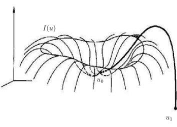
I(u)
u1 u0
Figure 1.1: The Mountain Pass Geometry.
Theorem 1.3.4 (Mountain Pass) Let B be a Banach space and I ∈ C1(B, R).
Suppose that there exist u0, u1∈ B and α, r > 0 such that
(MP1) infku−u0k=rI(u) ≥ α > I(u0);
(MP2) ku1k > r and I(u1) ≤ I(u0).
1.4 The Perron method 7
(i) I(un) → c, where
c := inf γ∈˜Γ max t∈[0,1]I(γ(t)) ˜ Γ = {γ ∈ C([0, 1], B) : γ(0) = u0, γ(1) = u1} (ii) I0(un) → 0 strongly in B∗.
If the functional I satisfies the (P S)c condition, then the number c, defined
above, is a critical level of I.
1.4
The Perron method
In this thesis, we will use the Perron method to solve some questions of ex-istence of solutions of a Dirichlet problem in a bounded domain, see Section 2.2.1. For more details about the Perron’s method we recommend to refer to the book [29].
In the Perron method the study of boundary behaviour of the solution, separated from the existence problem, is connected to the geometric prop-erties of the boundary through the concept of barrier function.
Definition 1.4.1 Let f be a function belonging to C0(Ω) and ξ a point of
∂Ω. Then f = fξ is called a barrier at ξ relative to Ω if: (i) f is superharmonic in Ω;
(ii) f > 0 in Ω − ξ; f (ξ) = 0.
Definition 1.4.2 A boundary point will be called regular if there exists a
barrier at that point.
Theorem 1.4.3 The classical Dirichlet problem in a bounded domain is
solvable for arbitrary continuous boundary values if and only if the boundary points are all regular.
1.5
A monotonicity result
The next result, due to H.Berestycki, L.Caffarelli and L.Nirenberg, [11], is about the monotonicity in some directions of positive solutions of elliptic second order boundary value problems of the type:
∆u + f (u) = 0 in Ω; u > 0 in Ω; u = 0 on ∂Ω, (1.11)
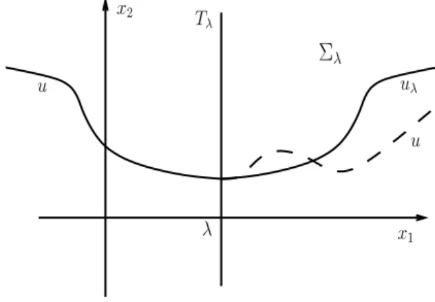
in the case that Ω is a slab domain. Such result will be useful in Chapter 3 to prove the nonexistence of solutions of boundary value problems like (3.33).
Theorem 1.5.1 ([11]) Let u be a solution of (1.11) in a slab Ω = Rn−1× (0, h),
n ≥ 2, satisfying
u(x, 0) = 0, ∀x ∈ Rn−1. (1.12)
Assume that f is Lipschitz and that
f (0) ≥ 0. (1.13)
Then,
∂u
∂y(x, y) > 0, ∀x ∈ R
n−1, ∀y ∈ (0, h/2). (1.14)
1.6
Some useful results about the least-energy
so-lutions to a semilinear perturbed Neumann
problem
In this section we collect a couple of useful results that we will use in Chap-ter 3.
Let us consider the following problem: −ε2∆u + u = f (u) in Ω; ∂u ∂ν = 0 on ∂NΩ; u > 0 in Ω. (1.15)
Moreover denote uε(Pε) = maxx∈Ωuε(P ) and H(·) the mean curvature of
the boundary ∂NΩ. The next result was proved by W.M.Ni and I.Takagi in
[49].
Theorem 1.6.1 (Ni-Takagi) Let uεbe a least-energy solution to the prob-lem (1.15) with f (u) = up, p ∈ (1,n + 2
n − 2) if n ≥ 3 and p ∈ (1, +∞) if n = 2. Suppose also that there exists P0 ∈ ∂NΩ such that
Pε → P0 ∈ ∂NΩ. Then ˜ Iε(uε) = εn ½ 1 2I(U ) − (n − 1)εγH(Pε) + o(ε) ¾ as ε → 0
where U is the ground state solution of problem (1.1), ˜Iε(·) the Euler func-tional associated to this problem (1.2), and γ a constant given by
γ := 1 n + 1 Z Rn + U0(|z|)zndz > 0.
1.7 The Lax-Milgram lemma 9
The following technical result was proved by C.S.Lin, W.M.Ni and I.Takagi in [38].
Lemma 1.6.2 (Li-Ni-Takagi) Let us consider the problem (1.15).
As-sume that the function f : R → R is of class C1(R) and satisfies the following
classical assumptions: (i) f (t) ≡ 0 for t ≤ 0;
(ii) f (t) = O(tr) as t → +∞, with: 2 < r + 1 < n−22n if n ≥ 3, r > 1 if n = 2; (iii) f (t)
t is increasing for t > 0 and limt→+∞ f (t)
t = +∞, while f (t) = o(t) for t → 0;
(iv) there exists a constant θ > 2 such that 0 < θF (t) ≤ tf (t) for t ≥ 0, where F (t) is defined by
F (t) :=
Z t
0
f (s)ds.
Moreover let uε be a solution to the problem (1.15). Then
Z
Ω
urεdx ≤ Crεn,
where Cr is a constant independent of ε and r any exponent greater than zero.
Next result, proved by W.M. Ni and I.Takagi, locates the maximum point
Pε on the boundary. Indeed it shows that H(Pε), the mean curvature of ∂Ω
at Pε, approaches the maximum of H(P ) over ∂Ω as ε → 0.
Theorem 1.6.3 Let uε be a least-energy solution to problem (1.15) and Pε∈ ∂Ω be the unique point at which max uε is achieved. Then
lim
ε→0H(Pε) = maxP ∈∂ΩH(P ), where H(P ) denotes the mean curvature of ∂Ω at P.
1.7
The Lax-Milgram lemma
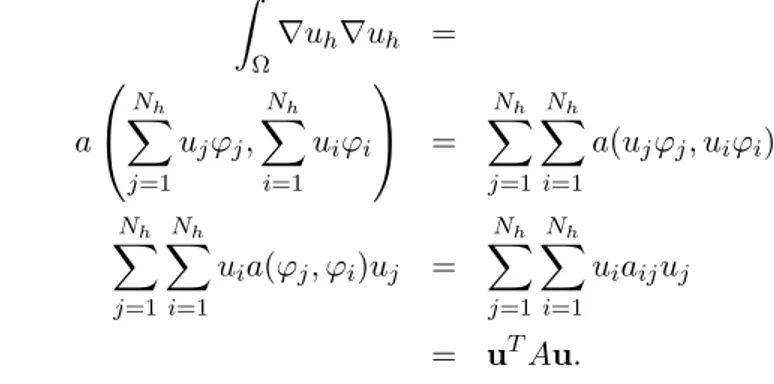
In this section we state a very useful lemma that we will utilize in Chapter 4 in connection with the weak formulation of some elliptic problem. Let there be given a normed vector space V with norm || · ||, a continuous bilinear form a(·, ·) : V × V → R and a continuous functional f : V → R.
Lemma 1.7.1 (Lax-Milgram) Let V be a Hilbert space, let a(·, ·) : V ×
V → R be a continuous coercive bilinear form and let f : V → R be a continuous linear form.
Then the abstract variational problem: Find an element u such that u ∈ V and ∀v ∈ V, a(u, v) = f (v), (1.16)
has one and only one solution.
By this theorem one can affirm that the variational problem (1.16) is well-posed in the sense that its solution exists, is unique and depends continu-ously on the data f , all other data being fixed.
1.8
Notations
In this section we will introduce some notations used throughout this thesis. In what follows Ω will be an open bounded subset of Rn, n ≥ 2, with a
sufficiently smooth boundary ∂Ω. We will suppose that ∂Ω is union of two disjoint open subsets ∂DΩ and ∂NΩ. We will call IΩ the intersection of the
closures of ∂DΩ and ∂NΩ.
We will consider the usual Sobolev space H1
0(Ω), i.e. the closure of
C0∞(Ω) with respect to H1(Ω), endowed with the norm defined as follows
kuk = µZ Ω | ∇u |2 ¶1 2 .
We will also use the Sobolev space H1
D(Ω), i.e. the family of functions
belonging to H1(Ω) with zero trace on ∂
DΩ.
Moreover ε > 0 will denote, throughout the thesis, a perturbation pa-rameter tending to zero.
Generic fixed constants will be denoted by C, and will be allowed to vary within a single line or formula. We will often use the notation d(1 + o(1)), where o(1) stands for a quantity which tends to zero as d → +∞.
Chapter 2
Concentration of solutions
and Perturbation Methods
In this chapter we study the asymptotic behavior of some solutions to a singularly perturbed problem with mixed Dirichlet and Neumann boundary conditions. In particular we are interested in the following problem −ε2∆u + u = up in Ω; ∂u ∂ν = 0 on ∂NΩ; u = 0 on ∂DΩ; u > 0 in Ω, ( ˜Pε)
where Ω is a smooth bounded subset of Rn, p ∈³1,n+2 n−2
´
, ε > 0 is a small parameter, and ∂NΩ, ∂DΩ are two subsets of the boundary of Ω such that the union of their closures coincides with the whole ∂Ω. We prove that, under suitable geometric conditions on the boundary of the domain, there exist solutions which approach the intersection of the Neumann and the Dirichlet parts as the singular perturbation parameter tends to zero. Denoting IΩthe
intersection of closures of ∂DΩ and ∂NΩ and assuming that the gradient of H at IΩ point toward ∂DΩ, the main result of this chapter is the following theorem.
Theorem 2.0.1 Suppose Ω ⊆ Rn, n ≥ 2, is a smooth bounded domain, and that 1 < p < n+2
n−2 (1 < p < +∞ if n = 2). Suppose ∂DΩ, ∂NΩ are disjoint open sets of ∂Ω such that the union of the closures is the whole boundary of
Ω and such that their intersection IΩ is an embedded hypersurface. Suppose
Q ∈ IΩ is such that H|IΩ is critical and non degenerate at Q, and that ∇H 6= 0 points toward ∂DΩ. Then for ε > 0 sufficiently small problem ( ˜Pε) admits a solution uε concentrating at Q.
Remark 2.0.2 (a) The non degeneracy condition in Theorem 2.0.1 can be
H|IΩ, or by the fact that there exists an open set V of IΩ containing Q such
that H(Q) < inf∂VH (respectively H(Q) > sup∂VH).
(b) With more precision, as ε → 0, the above solution uε possesses a unique global maximum point Qε ∈ ∂NΩ, and dist(Qε, IΩ) is of order ε log1ε
as ε tends to 0.
To prove Theorem 2.0.1, we will apply the perturbation methods in critical point theory. In the next section, we will start with an abstract outline to prove the existence of critical points of functionals, as in our case, that are perturbative.
2.1
The mixed perturbed problem
We are interested in finding solutions to ( ˜Pε) with a specific asymptotic
profile, so it is convenient to scale the variables like x 7→ εx and to study ( ˜Pε) in the dilated domain
Ωε := 1εΩ.
After this change of variables the problem becomes −∆u + u = up in Ω ε; ∂u ∂ν = 0 on ∂NΩε u = 0 on ∂DΩε; u > 0 in Ωε, (Pε)
where ∂NΩε and ∂DΩε stand for the dilations of ∂NΩ and ∂DΩ respectively. The Euler functional corresponding to (Pε) is the following
Iε(u) = 12 Z Ωε ¡ |∇u|2+ u2¢dx − 1 p + 1 Z Ωε |u|p+1dx; u ∈ HD1(Ωε), (2.1) where H1
D(Ωε) denotes the family of functions in H1(Ωε) with zero trace on ∂DΩε.
2.1.1 Perturbation in critical point theory
In this subsection, we introduce an abstract perturbation method which takes advantage of the variational structure of the problem, allowing to reduce it to a finite dimensional one. In particular we start treating existence of critical points for a class of functionals which are perturbative in nature. Given a Hilbert space H (which might depend on the perturbation pa-rameter ε), we want to consider manifolds embedded smoothly in H, pre-cisely for which
i) there exists a smooth d-dimensional manifold Zε⊆ H and C, r > 0 such
that for any z ∈ Zε, the set Z ∩ Br(z) can be parameterized by a map
2.1 The mixed perturbed problem 13
We are also interested in functionals Iε: H → R of class C2,α which satisfy
the following properties
ii) there exists a continuous function f : (0, ε0) → R with limε→0f (ε) = 0
such that kI0
ε(z)k ≤ f (ε) for every z ∈ Zε: moreover we require that kI00
ε(z)[q]k ≤ f (ε)kqk for every z ∈ Zε and every q ∈ TzZε;
iii) there exist C, α ∈ (0, 1], r0 > 0 such that kIε00kCα ≤ C in the subset
{u : dist(u, Zε) < r0};
iv) letting Pz, z ∈ Zε, denote the projection onto the orthogonal
comple-ment of TzZε, there exists C > 0 (independent of z and ε) such that PzIε00(z), restricted to (TzZε)⊥, is invertible from (TzZε)⊥ into itself,
and the inverse operator satisfies k(PzIε00(z))−1k ≤ C.
First some notation is in order. Let us set W = (TzZε)⊥and let (qi)1≤i≤d
be an orthonormal d-tuple (locally smooth on Zε) such that
TzZε= span{q1, . . . , qd}.
In the sequel we will denote by z = zξ, ξ ∈ Rd, a smooth local
parameteri-zation of Zε as in i). Furthermore, we also suppose that qi = ∂ξizξ/k∂ξizξk
at a given point of Zε.
We will look for critical points of Iε in the form u = z + ω with z ∈ Zε and ω ∈ W . If Pz : H → W is as in iv), the equation Iε0(z + ω) = 0 is
equivalent to the system ½
PzIε0(z + ω) = 0 (auxiliary equation);
(Id − Pz)I0
ε(z + ω) = 0 (bifurcation equation).
(2.2) Proposition 2.1.1 Let i)-iv) hold true. Then there exists ε0 > 0 with the following property: for all |ε| < ε0 and for all z ∈ Zε, the auxiliary equation in (2.2) has a unique solution ω = ωε∈ W = (TzZε)⊥, which is of class C1 with respect to z ∈ Zεand such that kωε(z)k ≤ C1f (ε) as |ε| → 0, uniformly with respect to z ∈ Zε. The derivative of ω with respect to z, ω0ε, satisfies the bound kω0
ε(z)k ≤ CC1f (ε)α.
Proof. The proof is a refinement of a (by now) standard argument, which can be found for example in [2], Section 2: since however the procedure is rather short, we write here the details for the reader’s convenience.
Property iv) allows us to apply the contraction mapping theorem to the auxiliary equation. In fact, by the invertibility of PzIε00(z) we can rewrite it
tautologically as ω = −(PzIε00(z))−1 £ PzIε0(z) + ¡ PzIε0(z + ω) − PzIε0(z) − PzIε00(z)[ω] ¢¤ := Gε,z(ω).
We claim next that the latter map is a contraction on a suitable metric ball of W . In fact, for the second term of Gε, using iii) we can write that
° °PzIε0(z + ω) − PzIε0(z) − PzIε00(z)[ω] ° ° = ° ° ° °Pz Z 1 0 (Iε00(z + sω) − Iε00(z))[ω]ds ° ° ° ° ≤ Ckωk1+α, and therefore by ii) and iv) we have
kGz,ε(ω)k ≤ Cf (ε) + C2kωk1+α; kωk ≤ r0.
Similarly, one also finds
kGz,ε(ω1) − Gz,ε(ω2)k ≤ C2(kω1kα+ kω2kα)kω1− ω2k.
By the last two equations, if we fix C1> 0 sufficiently large and let
Bε= {ω ∈ W : kωk ≤ C1f (ε)},
we can check that Gz,εis a contraction in Bε, so for every z ∈ Zεwe obtain a
(unique) function ω satisfying the required bound (for brevity, in the sequel the dependence on z will be assumed understood).
Let us now show that also the derivatives of ω with respect to ξ can be controlled by means of f (ε). Indeed, for the components of ω tangent to Zε
we can argue as follows: since (ω, ∂ξz) = 0 for every ξ, differentiating with
respect to ξ we find that (∂ξω, ∂ξz) = −(ω, ∂ξ2z). Since kωk = O(f (ε)) and
since ∂2
ξz is bounded (by i)), the tangent components of ∂ξω are bounded
in norm by CC1f (ε).
About the normal components, we can differentiate the relation
I0
ε(z + ω) =
Pd
i=1αi∂ξiz (where αi ∈ R) with respect to ξ to find
Iε00(z + ω)[∂ξz] + Iε00(z + ω)[∂ξω] = d X i=1 (∂ξαi)∂ξiz + d X i=1 αi∂ξξ2iz. (2.3) Since I00
ε is locally H¨older continuous (by iii)) and since kωk = O(f (ε))
projecting on W , for ε small by iv) we have that
kPz∂ξωk ≤ C|α| + CkIε00(z)[∂ξz]k + Ckωkα ≤ Cf (ε)α.
For the latter inequality we used again kωk = O(f (ε)) together with the Lipschitzianity of I0
ε (which imply |α| ≤ Cf (ε)) and ii).
Remark 2.1.2 From formula (2.3), writing I00
ε(z+ω) as (Iε00(z+ω)−Iε00(z))+ Iε00(z) and using ii), one finds the following more precise estimate
kPz∂ξωk ≤ Cf (ε) + Ck(Iε00(z + ω) − Iε00(z))[∂ξz]k.
Under further regularity assumptions on ω, the estimate of kPz∂ξωk can be improved: this will be useful for us to treat the case p ∈ (1, 2), see the proof of Proposition 2.3.5.
2.1 The mixed perturbed problem 15
We shall now provide conditions for solving the bifurcation equation in (2.2). In order to do this, let us define the reduced functional Iε : Z → R by setting
Iε(z) = Iε(z + ωε(z)). (2.4)
Proposition 2.1.3 Suppose we are in the situation of Proposition 2.1.1,
and let us assume that Iε has, for |ε| sufficiently small, a stationary point zε: then uε = zε+ ωε(zε) is a critical point of Iε. Furthermore, there exist
˜c, ˜r > 0 such that if u is a critical point of Iε with dist(u, Zε,˜c) < ˜r, where Zε,˜c= {z ∈ Zε : dist(z, ∂Zε) > ˜c} ,
then u has to be of the form zε+ ωε(zε) for some zε∈ Zε.
Proof. The first assertion can be proved as follows. Consider the manifold ˜
Zε = {z + ωε(z) : z ∈ Zε}. If zε is a critical point of Iε, it follows that
uε= zε+ ω(zε) ∈ ˜Zε is a critical point of Iε constrained on ˜Zε and thus uε
satisfies I0
ε(uε) ⊥ TuεZ˜ε. Moreover the definition of ωε, see Proposition 2.1.1,
implies that I0
ε(uε) ∈ TzεZε. Since, for |ε| small, TuεZ˜ε and TzεZε are close,
which is a consequence of the smallness of ω0ε, it follows that Iε0(uε) = 0.
To prove the last statement it is sufficient to notice that the contraction argument in the proof of Proposition 2.1.1 can be performed in the larger ball
˜
B = {ω ∈ W : kωk ≤ 2˜r} with ˜r sufficiently small, so one has uniqueness of
the solution of the auxiliary equation in this set. The distance condition on
Zε,˜c ensures the full applicability of these arguments in {dist(u, Zε,˜c) < ˜r},
so the conclusion follows.
2.1.2 Approximate solutions for (Pε) with Neumann
condi-tions
In this subsection we exhibit a family of (known) functions which satisfy the equation in (Pε) up to an error of order ε2, and whose normal boundary
derivative vanishes, up to the same order. After, introducing some conve-nient coordinates which stretch the boundary, we recall some results from [2] concerning approximate solutions to the Neumann problem. Then, using a further change of variables which also stretches the interface, we modify these functions conveniently for our purposes.
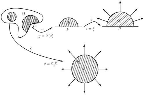
Let us describe ∂Ωε near a generic point Q ∈ ∂NΩε. Without loss of
generality, we can assume that Q = 0 ∈ Rn, that {x
n = 0} is the tangent
plane of ∂Ωε(or ∂Ω) at Q, and that ν(Q) = (0, . . . , 0, −1), where ν(Q) stands for the outer unit normal at Q. In a neighborhood of Q, let xn= ψQ(x0) be
a local parametrization of ∂Ω, x0∈ Rn−1. Then on ∂Ω one has
where AQ is the Hessian of ψ at 0, and where µ0 is some small number
depending on Ω. We have clearly H(Q) = n−11 trAQ. On the other hand, ∂Ωε is parameterized using the function ψQε(x0) := 1εψQ(εx0), for which the
following expansions hold
ψQε(x0) = ε 2hAQx
0, x0i + ε2O(|x0|3);
(2.6)
∂iψεQ(x0) = ε(AQx0)i+ ε2O(|x0|2).
Concerning the outer normal ν, we have also
ν = ³∂ψε Q ∂x1, . . . , ∂ψε Q ∂xn−1, −1 ´ ³ 1 + |∇ψε Q|2 ´1 2 =¡ε(AQx0), −1¢+ ε2O(|x0|2). (2.7)
Since ∂Ωε is almost flat for ε small and since the function U (see the
Introduction) is radial, for Q ∈ ∂Ωε we have ∂ν∂ U (· − Q) ∼ 0. Thus U (· − Q)
is an approximate solution to (Pε) if we impose pure Neumann boundary conditions. Hence for the latter problem a natural choice of the manifold Zε
(see Subsection 2.1.1) could be the following
Zε= {U (· − Q) := UQ : Q ∈ ∂Ωε} .
Indeed we need a more accurate expansion, and we will construct better ap-proximate solutions, in particular improving the condition at the boundary. Given µ0 as in (2.5), we introduce a new set of coordinates on Bµ0
ε (Q) ∩ Ωε.
Let
˜
x0= x0; x˜n= xn− ψQε(x0). (2.8)
The advantage of these coordinates is that ∂Ωε identifies with {˜xn = 0},
but the corresponding metric coefficients ˜gij will not be constant anymore.
From (2.6) it follows that ˜
gij = Id + εAQ+ O(ε2|˜x0|2); ∂x˜k(˜gij) = ε∂x˜kAQ+ O(ε2|˜x0|), (2.9)
with AQ= µ 0 AQx˜0 (AQx˜0)t 0 ¶ .
Here the zero in the upper left corner of AQ stands for the trivial (n −
1) × (n − 1) matrix, while (AQx˜0)t stands for the transpose of the column
vector (AQx˜0). It is also easy to check that the inverse matrix (˜gij) is of the
form ˜gij = Id − εAQ+ O(ε2|˜x0|2), and that ∂ ˜
xk(˜gij) = −ε∂x˜kAQ+ O(ε2|˜x0|).
Moreover, by the expression of the coordinates ˜x one has
2.1 The mixed perturbed problem 17
Recall that the Laplacian with respect to a general metric is given by ∆gu = √ 1 det g∂j ³ gijpdet g ´ ∂iu + gij∂ij2u,
so in our situation, by (2.10), we get
∆gu = gijuij + ∂i(gij)∂ju.
Using (2.9) we find that, formally ∆˜gu = ∆Rnu − ε
¡
2hAQx˜0, ∇x˜0∂˜xnui + (trAQ)∂x˜nu
¢
+ O(ε2)(|∇u| + |∇2u|).
(2.11) We also give the expression of the unit outer normal to ∂Ωε, ˜ν, in the new
coordinates ˜x. Letting νi (resp. ˜νi) be the components of ν (resp. ˜ν), from ν =Pni=1νi ∂ ∂xi = Pn i=1ν˜i ∂∂ ˜xi, we have ˜νk= Pn i=1νi ∂ ˜x k ∂xi. This implies ˜ νk= νk, k = 1, . . . , n − 1; ν˜n= n−1 X i=1 νi∂ψ ε Q ∂ ˜xi + νn.
From (2.6) and the subsequent formulas we find ˜
ν =¡εAQx˜0, −1
¢
+ ε2O(|˜x0|2). (2.12) Finally the area-element of ∂Ωε can be expanded as
dσ = (1 + O(ε2|˜x0|2))d˜x0. (2.13) Linearizing the equation in (Pε) near U (˜x), one sees that the function U (y)+ εw(y) solves the equation (Pε) up to an error o(²), if w satisfies
½ LUw = −2hAQx˜0, ∇x˜0∂x˜nU i − (trAQ) ∂x˜nU in Rn+; ∂ ∂ ˜xnw = hAQx˜ 0, ∇ ˜ x0U i on ∂Rn+.
Therefore, if wAQ is given by Lemma 1.2.2 (see Chapter 1) with T = AQ,
one sees that, formally at least, the accuracy of the solution improves. To derive rigorous estimates in this spirit, one can choose a cut-off function χµ0 on Rn with the properties
χµ0(˜x) = 1 in Bµ0 4 ; χµ0(˜x) = 0 in Rn\ Bµ02 ; |∇χµ0| + |∇2χµ0| ≤ C in Bµ02 (Q) \ Bµ04 , (2.14)
and for any Q ∈ ∂Ω define the following function, in the coordinates (˜x0, ˜x n) zε,Q(˜x) = χµ0(ε˜x)(U (˜x) + εwAQ(˜x)). (2.15)
The next result collects estimates in the statements and the proofs of Lem-mas 1.2.3, 1.2.4 and 1.2.5 in Subsection 1.2.4.
Proposition 2.1.4 There exist constants C, K > 0, depending only on p,
n and Ω such that for ε small the following estimates hold
¯ ¯ ¯ ¯∂z∂ ˜ε,Qν ¯ ¯ ¯ ¯ (˜x0) ≤ ( Cε2(1 + |˜x0|K)e−|˜x0| for |˜x0| ≤ µ0 4ε; Ce−Cε1 for µ0 4ε ≤ |˜x0| ≤ µ2ε0, ¯ ¯ ¯−∆gzε,Q+ zε,Q− zε,Qp ¯ ¯ ¯ (˜x) ≤ ( Cε2(1 + |˜x|K)e−|˜x| for |˜x| ≤ µ0 4ε; Ce−Cε1 for µ0 4ε ≤ |˜x| ≤ µ2ε0, Iε,N(zε,Q) = ˜C0− ˜C1εH(εQ)+O(ε2); ∂Q∂ Iε,N(zε,Q) = − ˜C1ε2H0(εQ)+o(ε2), where ˜ C0 = µ 1 2 − 1 p + 1 ¶ Z Rn + Up+1dx, C˜1 = µZ ∞ 0 rnUr2dr ¶ Z Sn + yn|y0|2dσ.
To improve the estimate, we need to take into account the effect of the Dirichlet boundary condition. To this end, we make next a further change of variables, in order to stretch also the interface: we claim indeed that, in the coordinates ˜x, the latter can be parameterized as ˜x1 = d + ˜ψε
Q( ˜x00),
˜
x00 = (˜x
2, . . . , ˜xn−1), with d ∈ R and ˜ψQε satisfying estimates similar to
(2.6). To see this, we first claim that the curvature of the interface IΩε, in
the coordinates ˜x, is of order O(ε). Here we are assuming that the distance
of Q from IΩε, multiplied by ε, is bounded by a small constant depending
on Ω. For showing this, let us consider a curve γ(s) in the interface whose geodesic curvature (relative to IΩε) vanishes and which is parameterized
by arclength: its curvature in Rn will be therefore of order O(ε). Let us
split γ into its tangent and normal components (with respect to TQ∂Ωε) γ = (γT, γN). Since in our notation γN = ψε
Q(γT), from (2.6) and a Taylor
expansion we have that
| ˙γ|2= | ˙γT|2+ | ˙γN|2 ⇒ | ˙γ| = | ˙γT|(1 + O(ε2)|γT|2). The curvature of γ is k = 1 | ˙γ|dsd ³ ˙γ | ˙γ| ´
, which can be written as
k = (1 + O(ε2)|γT|2) | ˙γT| d ds µ ˙γT | ˙γT|(1 + O(ε2)|γT|2) ¶ .
Expanding the above expression we obtain
k = kT(1 + O(ε2)|γT|2) + O(ε2)|γT|.
This formula shows that, since k is of order ε, also kT is of order ε. Therefore,
if the point Q is close to the interface (in the sense specified before) and if we choose the ˜x1 axis to be perpendicular to the projection of IΩε onto TQ∂Ωε,
2.1 The mixed perturbed problem 19
if the latter projection is at distance d from Q we have that the points in
IΩε satisfy
˜
x1 = d + ˜ψεQ(˜x00); x˜00= (˜x2, . . . , ˜xn−1), (2.16)
where ˜ψεQ (which depends on Q and ε) is such that ˜
ψε(0) = 0; ∇ ˜ψε(0) = 0; ψ˜εQ(˜x00) =
1 2εh ˜AQx˜
00, ˜x00i + O(ε2|˜x00|2),
see also (2.6). Below, it will be always understood that the symbol d refers to the distance to the scaled interface IΩε and we will never use subscript ε
to stress this fact.
Introducing the new coordinates
y1= ˜x1− ˜ψεQ(˜x00); y00= ˜x00; yn= ˜xn, (2.17)
we have that the metric coefficients gy satisfy again
det gy ≡ 1, (2.18)
as in (2.10). Then, similarly to (2.9) we have that
gyij = Id + ε ˜AQ+ O(ε2|y0|2); ∂yk(g
y
ij) = ε∂ykA˜
Q+ O(ε2|y0|) (2.19)
(and similarly (gy)ij = Id − ε ˜AQ + O(ε2|y0|2), ∂yk(gy)ij = −ε∂ykA˜Q +
O(ε2|y0|)), where ˜ AQ= 0 ( ˜AQy 00)t A Qy0 ˜ AQy00 0 (AQy0)t 0 .
Remark 2.1.5 (a) We stress that, in the new coordinates y, the origin
parameterizes the point Q on ∂Ω, and that functions decaying as |y| → +∞ will concentrate near Q.
(b) It is also useful to understand how the metric coefficients gyij vary with Q. Notice that in (2.19) the deviation from the Kronecker symbols is of order ε, and that we are working in a domain scaled of 1ε, so a variation of order 1 of Q corresponds to a variation of order ε in the original domain. Therefore, a variation of order 1 in Q yields a difference of order ε2 in gy
ij, and precisely
∂gijy
∂Q = O(ε
2|y0|2),
with a similar estimate for the derivatives of the inverse coefficients (gy)ij. For more details see the end of Subsection 9.2 in [2].
From the latter formulas, the counterpart of (2.11) becomes ∆gyu = ∆Rnu − ε ¡ 2hAQy0, ∇y0∂ynui + (trAQ)∂ynu ¢ − ε ³ 2h ˜AQy00, ∇y00∂y1ui + (tr ˜AQ)∂y1u ´ + O(ε2)¡|∇yu| + |∇2yu| ¢ , (2.20)
while the analogues of (2.12) and (2.13) are
νy =¡εAQy0, −1
¢
+ ε2O(|y0|2); dσy = (1 + O(ε2|y0|2))dy0. (2.21) Reasoning as for the above coordinates ˜x (see the comments after (2.13)),
one sees that the function U (y) + ε ˜w(y) solves the equation in (Pε) up to an
error o(ε) if and only if ˜w satisfies
LUw = −2hA˜ Qy0, ∇ y0∂ynU i − (trAQ) ∂ynU − 2h ˜AQy00, ∇y00∂y1U i − (tr ˜AQ) ∂y1U in Rn+; ∂ ∂ynw = hA˜ Qy 0, ∇ y0U i on ∂Rn+. (2.22)
We have an explicit solution to (2.22) in terms of the above function wAQ
through a simple change of variable. Indeed, in the new coordinates y we can write that formally
zε,Q(˜x) ' U ³ y1+ε2h ˜AQy00, y00i, y00, yn ´ + εwAQ ³ y1+ε2h ˜AQy00, y00i, y00, yn ´ ' U (y) + ε 2h ˜AQy 00, y00i∂
1U (y) + εwAQ(y) + o(ε).
Choosing ˜w(y) = ˜wQ(y) := 1
2h ˜AQy00, y00i∂1U (y) + wAQ(y) and using the fact
that LU∂yiU (y) = 0, from an explicit computation we find that
LUw˜Q(y) = LUwAQ(y) − (tr ˜AQ)∂1U (y) + 2h ˜Ay00, ∇y00∂1U (y)i,
which is exactly the desired equation. Clearly, by (1.10), there exists a constant C0
Ω, depending on Ω and on the curvatures of the interface such
that
| ˜wQ(y)| + |∇ ˜wQ(y)| + |∇2w˜Q(y)| ≤ CΩ0 (1 + |y|K)e−|y|. (2.23)
In conclusion, choosing a cutoff function as in (2.14) and defining the new approximate solution zε,Q as
zε,Q(y) = χµ0(εy) (U (y) + ε ˜wQ(y)) , (2.24) the arguments for the proof of Proposition 2.1.3 yield the following variant of the above result.