A variational treatment of hydrodynamic and magnetohydrodynamic flows

(1)

A variational treatment of hydrodynamic and

magnetohydrodynamic flows

by

Tommaso Andreussi

Classe di Scienze

Perfezionamento in

Matematica per la Tecnologia e l’Industria

SCUOLA NORMALE SUPERIORE November 2007

Thesis Supervisors:

(2)

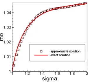
In order to describe stationary plasma flows in thrusters based on plasma propulsion, an ideal, axial symmetric, single-fluid motion is assumed. The conservation laws of conductive fluids and the Maxwell’s equations lead to a second order diﬀerential equation for the magnetic flux function ψ, i.e. the generalized Grad Shafranov (GS) equation, and to two implicit constraints relating ψ to the plasma density and the azimuthal velocity. This set of three equations, one diﬀerential and two algebraic, is then expressed using a variational approach and the solution is obtained in a straightforward manner from the extremum of the appropriate Lagrangian func-tional. The numerical approach is based on Ritz’s method, which has the advantage of producing analytic (though approximate) solutions. Both non-conductive fluids, where the acceleration can only be obtained exploiting the internal energy of the flow (thermodynamic process), and conductive fluids, where the electromagnetic forces play a fundamental role, are considered. In order to apply this approach to the acceleration processes in nozzle-like configurations, an open-boundary geometry is investigated and specific attention is paid to a physical definition of boundary conditions. Hydrodynamic shocks are taken into account and it is shown that the appropriate jump conditions follow implicitly from a natural extension of the Lagrangian variational principle. A comparison test with an explicit solution permits an estimate of the approximate results.

(5)

Introduction

Spacecraft propulsion outside the earth’s atmosphere is normally obtained by ejecting a pro-pellant fluid. The thrust is the product of the mass flow rate times a mean speed of the ejected flow. The amount of propellant, which greatly influences the cost, must be calculated based on a value estimated for this characteristic velocity. There are, however, chemical and thermo-dynamics constraints that limit the expansion of the combusted propellant beyond some speed levels. Electrically charged fluids, and in particular plasmas, have been considered over the last few decades, as they are subject to electromagnetic interactions. These interactions allow us to go beyond the limits of thermodynamics since other forces can be used in order to accelerate the propellant. This is why it has become important to understand the fundamentals of plasma dynamics in space propulsion.

In order to investigate thrust generation we exploit the fact that a non-charged fluid can be accelerated in a suitably shaped nozzle by letting it expand adiabatically. In this process a fraction of the internal energy of the fluid goes into kinetic energy, increasing the exit velocity. This fraction is related to the thermodynamic eﬃciency of the expansion and to the losses that prevent a full expansion. In spite of such a simple principle, the theory of de Laval nozzles (1890) is complex even for ideal fluids, where dissipative phenomena are neglected. The simplest way of studying this problem is that of assuming a steady state and a one-dimensional motion, whilst considering the section change in the conduit. Even with such simple assumptions, fluid dynamics equations are non-linear, and heavily influenced by a characteristic factor, the ratio of fluid speed to sound speed, the latter being the speed of propagation of changes in fluid properties. This ratio is named the Mach number, and the factor ¡M2_{− 1}¢ appearing in de Laval’s model causes a change in flow behaviour when going from subsonic regimes (M < 1) to supersonic ones (M > 1). It can be shown that, to accelerate the fluid, the nozzle section must

(6)

decrease along the axis in subsonic conditions, whilst it must increase in supersonic conditions. De Laval’s theory, though very simplified, allowed a good understanding of the fundamental phenomena and has led to the first supersonic nozzles (convergent-divergent).

For a short historical background, the equations governing ideal hydrodynamics were written by Euler in 1775 and have not been solved in the general case so far. The achievements in hydrodynamics in the two centuries from its first formulation have been slower than in other fields of theoretical physics. Euler’s theory allows us to decrease the number of unknown functions to deal with, but the equations remain quite complex. In the same period (in the years 1772-1788) J. L. Lagrange built the foundations of variational calculus, and showed its applications in classical mechanics and in fluid dynamics [17]. After the widespread introduction of variational calculus, in the early twentieth century, methods were introduced in order to solve variational problems directly. In particular, in 1907 Ritz proposed a fundamental method based on variational formulation [27].

Variational principles and their numerical applications have shown their power in handling hydrodynamics problems, in both the Eulerian and the Lagrangian descriptions. First attempts to define an Eulerian version of Hamilton’s principle were only partly eﬀective, as some over-simplifications were required for the equations of an ideal fluid. The starting point for these attempts was a transformation suggested by Clebsch [5] in 1859 of the hydrodynamics equa-tions. In 1929 Bateman [2] showed a variational formulation of fluid dynamics that allowed the derivation of Clebsch’s equations (Clebsch handled only an incompressible and isentropic fluid, but Lamb [18] included the simple extension of density change). This work, and the successive developments of Eckart [7], assumed the process to be isentropic. In addition, there was no connection between the functional used as a Lagrangian in [2][7] and the Hamilton’s principle. The first general Eulerian formulations of Hamilton’s principle were due to Lin [21] and Seliger & Whitham [31]. Starting from the Hamilton’s principle for the Eulerian descrip-tion and requiring the mass and entropy conservadescrip-tion by Lagrangian multipliers, Lin noticed that the solutions were limited to a subset of the general case and that additional constraints were necessary. To do so he added the conservation of the starting location of fluid particles (three components). These constraints, as shown by Bretherton [3], were forcing the equivalence between the Eulerian description of Hamilton’s principle and the one based on Lagrangian

(7)

de-scription. In Selinger & Whitham’s work the former achievements are clarified and settled down; also, the constraints implicit in the Eulerian formulation (with a single Lin binding coordinate required) become explicit and their correctness is proved (i.e. the equivalence of Clebsch’s transformations to Euler’s general equations). Moreover the same formulation is compared to the variational theory of electromagnetism and extended to plasma dynamics and to elasticity. Then, Broer & Kobussen [4] and Van Saarlos [35] showed that the formulations of Bateman and Lin may be obtained directly from the Lagrangian description by canonical transforma-tions. After Lagrange’s achievements, the Lagrangian version of Hamilton’s principle has been extended to theoretical fluid dynamics by many authors. The work by Salmon [29] shows, as an example, how to model fluid behaviour at geophysical scales with this method.

In the case of plasma, things are more complex, partly because the theory is more recent (the first works are due to Thomson (1897) and Langmuir (1927)), but mainly because of the tight interaction between the dynamic and the electromagnetic eﬀects in the fluid. A plasma may be described as a fluid containing a non-negligible amount of free charged particles, which allow for electromagnetic forces, capable of acting at non-contact distances, to influence the local behaviour of the fluid. As an example, such interactions allow for treating a rarefied gas as a fluid, even when that treatment would otherwise be incorrect. On the other hand, in spite of the highly ionized state, the fluid may macroscopically behave as a non charged medium, though the behaviour as a continuum is a consequence of the long range electromagnetic interactions, which keep the fluid in a globally non-charged state. The theory based on these assumptions is named ideal magnetohydrodynamics (MHD). It reduces to Euler’s equations of classic hydrodynamics when electromagnetic phenomena are absent.

In order to deal with the ideal MHD, a first simplifying step has been made. When the plasma is stationary and there is axial symmetry, MHD equations may be transformed by the introduction of a scalar function ψ dependent on the flux of the poloidal magnetic field. This reduces the problem to a single partial derivatives diﬀerential equation, named after the work by Grad [11] and by Shafranov [33] (GS), who first derived it (sometimes referred to also as the equation of Grad-Shafranov\Lüst-Shlüter, from Lüst & Shlüter [24]). This equation was used for development work in the field of plasma-fusion and greatly contributed to the explanation of the first experiments. Many proposed configurations, the tokamak in the first place (Grad

(8)

& Rubin [11], Shafranov [33]), have been described in a first approximation using this model. The most eﬀective way to treat this problem mathematically is by calculus of variations. A variational formulation of hydromagnetic equilibrium conditions, including the velocity field, was extensively treated for the first time by Woltjer [37][36]. The procedure is to bound the energy of the system with a suﬃcient number of constraints, but the equations that describe these constraints are treatable only in the axisymmetric case. In the same line of action as GS and restraining the analysis to the axisymmetric case, Heinemann & Olbert [14] in 1978 derived a single equation describing the equilibrium of ideal MHD flows and proposed a variational principle useful to simplify the mathematical treatment.

Going from the stationary case to the conditions of steady state flow (_∂t∂ _{= 0, v 6= 0), it is} found that the system is governed by two coupled equations, one a generalized GS equation (a partial differential equation), the other a generalized Bernoulli equation for fluid dynamics (a non linear algebraic equation). The same structure is found for uncharged fluids, although much simpler because of the absence of the electromagnetic terms (see Scott & Lovelace [30]). A detailed description of the GS equations with a non-stationary fluid is given by Lovelace et al. [23]. They deal with the difficulties of the generalized differential GS equation, due particularly to the coupling of this non-linear equation with an implicit algebraic Bernoulli’s equation.

Because of these diﬃculties there is currently a wide interest in the variational description. Hameiri [13] demonstrated that, following the ideas present in the work by Woltjer, it is possible to derive a general (non-axisymmetric) variational principle for toroidal configurations. Also, an elegant variational description of MHD stationary flows is found in Goedbloed [8]. This simplified model is adopted in the problem treated here.

For simplicity, we first studied the behaviour of the non-charged fluids (dropping the Maxwell equations). The first part of each chapter is hence devoted to the hydrodynamics, whilst the second treats the plasma theory. The model that is developed here may be considered as quite limited, but, although it handles quasi-isentropic and axisymmetric stationary flows, it opens interesting views on astrophysical phenomena, fusion experiments and plasma propulsion.

The treatment for the model is explained in Chapter 1, whilst Chapter 2 is dedicated to the description of the numerical solution and to the analysis of the results. The numerical approach is systematically based on Rayleigh-Ritz’s method [27][28], which has the additional advantage

(9)

(10)

Chapter 1 Models

In spacecraft propulsion a fundamental task is the eﬃcient acceleration of the propellant fluid. By increasing the exhaust velocity and by generating a fast collimated jet it is possible to greatly improve the mission capabilities. Basically, the technical solution consists in expanding a highly compressed gas, typically the product of a chemical reaction, through a suitably shaped channel. To convert a considerable amount of internal energy into an eﬀective speed growth, the shape of the acceleration channel (nozzle) has been deeply investigated both in theory and experimentally [22]. The basic geometry, as suggested by the ideal gasdynamics, consist in a convergent part that increases the fluid velocity up to the speed of sound and then in a divergent part in which the supersonic flow reaches the maximum speed. The optimum shape of this second part is designed in order to avoid a shock transition to subsonic flow and by minimizing the flux beam divergence, that is to obtain a velocity direction as uniform as possible at every point of the outlet surface.

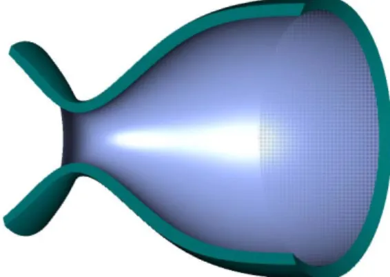
To further increase the propellant velocity and maintain the flux control, the interaction between conductive fluids, or plasmas, and electromagnetic fields have been exploited. Although the plasma acceleration processes present many diﬀerent possibilities with respect to the non-conductive gasdynamics, the use of a nozzle configuration like the one described here seems to improve the thrust performance. In this case, both an external coil and the plasma currents produce a magnetic field that is constrained by a conductive surface. This surface, typically shaped as a hyperboloid of revolution, defines the plasma acceleration channel. The plasma flow can be controlled and optimized by using the external magnetic coil. Due to the complex

(11)

Figure 1-1: Hydrodynamic nozzle

combination of hydrodynamic motion and electromagnetic fields, the main features of this process have been described in its essential aspects only [15].

1.1 Governing Equations

In his fundamental paper on ionized gases Langmuir writes: "Except near the electrodes, where there are sheaths containing very few electrons, the ionized gas contains ions and electrons in about equal numbers so that the resultant space charge is very small. We shall use the name plasma to describe this region containing balanced charges of ions and electrons"[20]. Langmuir’s model is important since, by considering spatial and time scales suﬃciently large, the ensemble of diﬀerent species of the plasma, ions and electrons, behave like that of a single, perfectly conducting, fluid.

The magnetohydrodynamic description of astrophysical plasma explains, for example, the behaviour of magnetosphere, the dynamo process inside the star nucleus, and the study of accretion disks and massive stars [23]. Many plasma phenomena have a technical importance for spacecraft propulsion [15], fused metal processing and MHD generators [16]. However, most of the technical applications of plasma dynamics are related to nuclear fusion research [9].

(12)

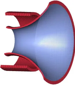
Figure 1-2: Magnetic nozzle

The MHD model, representing the starting assumption of this research, still permits a good approximation of the equilibrium state for fusion experiments.

Except for the magnetic force term in the momentum conservation law, Euler’s equations can be used to describe the steady flow of both an ideal fluid or a hydromagnetic medium as they provide a convenient approximation of the equations obtained by averaging the kinetic plasma equations.

The first assumption, made in this model, is to neglect all the dissipative phenomena, such as plasma resistivity and viscosity. This is in general admissible for high energy plasmas and yields a great simplification. More arbitrary is the subsequent assumption of an isotropic pressure tensor, since the local magnetic field direction deeply influences the particles’ motion. We leave the complexities of a non-isotropic model to a further development of this work.

In real applications these assumptions are not verified everywhere in the thruster but provide a very important first step in the investigation of the plasma dynamics.

Condition 1 Ideal steady flows.

(13)

time-derivative vanishes

∂ ∂t = 0, and mass conservation law becomes:

∇ · (ρv) = 0, (1.1)

where ρ and v represent the fluid density and velocity respectively. This equation holds for classical fluids, but also for other fluids employed in space propulsion, where there is no plasma generation or depletion. Considering the ionization process requires an additional source term in the right hand side of equation (1.1). However, since the plasma is assumed to be fully ionized before the inlet of the accelerating channel, equation (1.1) can be accepted.

The momentum equation for a fluid element

ρ(v · ∇)v | {z } inertial force = − _|{z}∇p pressure grad. + 1 cj× B | {z } , Lorentz force (1.2)

where p represents the isotropic pressure, expresses the fluid particle acceleration due to pressure gradient and, for conductive fluids, due to electromagnetic forces. This contribution, in non-relativistic regimes |v| ¿ c (with c denoting the speed of light), reduces to the Lorentz force term, the vectorial product of the current density j and the magnetic induction B. Compared with this term, the electrostatic acceleration can be neglected and space charge eﬀects may be dropped. Thus the plasma quasi-neutrality is assumed to hold:

ni ∼ neÀ (ni− ne) ,

where ni and ne represent the ion and the electron numerical density, that is the number of

particles for unit volume.

The last equation that determines the problem of non-conductive fluid motion, expresses the conservation of the entropy S (ρ, p) of each fluid element

(14)

This equation is obtained by using the equation of state of an ideal gas (with adiabatic index γ) and by neglecting the dissipation of fluid energy in microscopic phenomena, otherwise described by a resistivity and a viscosity term. We also notice that equation (1.3) does not imply that the entropy is everywhere the same, since, in general, entropy variations are allowed for fluid elements belonging to diﬀerent streamlines. These variations are determined by the initial non-equilibrium phase or, for flows passing through open domains, by the dissipative phenomena that may occur before the fluid entry. Assuming an isentropic motion for the fluid elements is a natural choice for the supersonic gas dynamics and is commonly adopted also for MHD.

In order to describe the motion of a perfectly conductive fluid interacting with a magnetic field, we need to combine the previous equations with Maxwell’s equations. This set of equations describes the evolution of the electric field E and the magnetic field B in response to the current density j. It is expressed by the following equations

∇ × B = 4π

c j (Ampere0s Law) , (1.4)

∇ × E = 0 (Faraday0s Law) , (1.5)

∇ · B = 0 (Magnetic Divergence0s Law) (1.6)

Since we decided to neglect the eﬀects of a space charge τ (x) ∝ (ni− ne), Poisson’s law

∇ · E = τ is no longer needed and may be dropped.

The last characteristic equation describing the electric field in a perfectly conducting moving medium is

E+ v× B

c = 0, (1.7)

which expresses that the electric field in a co-moving frame should vanish. In concrete terms, equation (1.7) represents Ohm’s law for a perfectly conductive fluid.

If a plasma must be confined by a rigid conductive boundary or by a magnetic field, it is most likely that there will be a transition region where the plasma properties adapt themselves

(15)

to the presence of boundaries or vacuum. The transition may be a sharp boundary or a gradual change in plasma quantities over some finite distance. In both cases it is necessary to match the variables for the solution of the model equations on adjacent sides of the transition region. Therefore the boundary conditions can be expressed in terms of the change of a plasma variable χ across the interface. The unit vector normal to the interface is denoted by n and the surface current in the boundary is denoted by js.

If we define

kχk = χi− χo (1.8)

the diﬀerence between the values assumed by χ on the two sides of the transition region, the boundary conditions result:

Plasma-plasma interface: ° ° ° °p + B2 8π ° ° ° ° = 0, n· kρvk = 0, n× kEk = n×kv × Bk_c = 0, n_{· kBk = 0,} n_{× kBk =} 4π c js. Plasma-perfectly conducting wall interface:

n_{· v = 0,} n_{× E = 0,} n_{· B = 0.}

The set of equations (1.1-1.7) and boundary conditions, or a part of them, can be used to describe diﬀerent problems. We focus our attention on three models of increasing complexity:

1. the static plasma problem (equation 1.2 without the inertial term, and equations 1.4-1.7); 2. the hydrodynamic problem (equations 1.1-1.3, excluding the Lorentz force term in

equa-tion 1.2);

3. the general plasma flow problem (the whole set, equations 1.1-1.7).

The first of these problems leads to the well known Grad-Shafranov equation and will not be reviewed in the following, while the other two will be discussed in the next sections.

(16)

Woltjer, in his papers on hydromagnetic equilibrium, writes: "Even if in the dynamics the assumption of axial symmetry is, in general, impermissible, it may be expected that most equi-librium configurations of interest will be axisymmetric" [36]. Thus, we study the axisymmetric dynamics of conductive and non-conductive fluids. This assumption is mainly due to the tech-nical importance and the resulting simpler model. In fact, this kind of symmetry is typically assumed as a project’s base not only in space propulsion research but also in fusion experiments. In what follows we use both spherical (σ, θ, φ) and cylindrical (r, φ, z) coordinates, on assuming that the solutions are independent of φ. This does not mean that the azimuthal velocity or magnetic field are zero.

Let us consider a vector field C that satisfies the divergence-free condition

∇ · C = 0

(in our case the mass flow ρv and the magnetic field B). A scalar function ψ independent on φ exists that defines the components of C in the symmetry plane (or poloidal plane φ = const) as

Cp = ∇ψ × ∇φ. (1.9)

The function ψ is typically named a stream-function since it has a constant value along the streamlines of the vector field to which it belongs, or a flux-function as it labels each stream surface with the flux of the vector fields that is enclosed in it.

1.1.1

Axisymmetric hydrodynamics

First we consider a non-conductive fluid. In this case Maxwell’s equations are not needed and the Lorentz force term in the momentum equation (1.2) can be dropped. The model reduces to the coupling of a partial diﬀerential equation and an algebraic constraint. In order to simplify these steps, we start assuming that the fluid entropy is uniform

(17)

Referring to flows passing through an open domain, this means that diﬀerent fluid elements enter, and exit, the domain with equal entropy. The modifications necessary to deal with entropy variations will be discussed later, at the end of this section.

Hereafter we also explicitly separate the poloidal fluid velocity vp from the azimuthal

com-ponent vφ = Ar, where A indicates the specific angular momentum per unit mass about the

symmetry axis.

Introducing the specific enthalpy h =R dp_ρ _{for the isentropic flow and the vorticity ω = ∇×v} of the fluid, equation (1.2) can be written in the form

v_{× ω = ∇B,} (1.10)

where B represents the Bernoulli ‘constant’

B = 1 2v 2 P + 1 2 A2 r2 + h (ρ) , (1.11)

that is conserved along stream and vortex lines.

In order to satisfy the mass conservation law (equation. 1.1) and the axisymmetry condition (equation. 1.9) we can define a stream function ψ such as

ρvz= 1 r ∂ψ ∂r ρvr= − 1 r ∂ψ ∂z (1.12)

or, in vectorial terms,

ρvp= ∇ψ × ∇φ.

By using the definition (1.12), equation (1.10) leads to the following expressions

B = B (ψ) A = A (ψ) ,

where the second equality is obtained again from the axial symmetry condition. Taking the curl of equation (1.10) yields the vorticity equation:

(18)

that is reduced by symmetry to: ρv · ∇ µ ωφ rρ ¶ = ∂ ∂z µ A2 r4 ¶ . (1.14)

A first integral of equation (1.14) can be obtained from the momentum equation, substitut-ing the definitions of ψ and ω:

ωφ rρ = A r2 dA dψ − dB dψ. (1.15)

Using the expression of ωφ in terms of ψ,

−rωφ= r ∂ ∂r 1 r µ 1 ρ ∂ψ ∂r ¶ + ∂ ∂z µ 1 ρ ∂ψ ∂z ¶ ,

we obtain a second order partial diﬀerential equation

r ∂ ∂r 1 r µ 1 ρ ∂ψ ∂r ¶ + ∂ ∂z µ 1 ρ ∂ψ ∂z ¶ = ρr2dB dψ−ρA dA dψ, (1.16)

for the stream function ψ. Inspection of this equation shows that for incompressible fluids (ρ = const) the problem is linear only if B (ψ) = b2ψ2 + b1ψ + b0 and A (ψ) = a1ψ hold. For

compressible fluids (ρ 6= const), the dependence of ρ on the stream function and its derivatives should be determined by using the Bernoulli equation

B (ψ) = 1 2 µ 1 r ∇ψ ρ ¶2 + 1 2 ∙ A (ψ) r ¸2 + γ γ − 1 p ρ, (1.17)

where the last term is obtained from the adiabatic constitutive equation of an ideal gas:

p ∝ ργ. This makes the diﬀerential problem non-linear.

In the case of non-uniform entropy propagation

v_{· ∇S = 0,} (1.18)

(19)

and p as S(ρ, p) = kB γ − 1 ∙ ln µ p ργ ¶ − ln µ p0 ργ₀ ¶¸ , (1.19)

where kBrepresents the Boltzmann constant and {ρ0, p0} are reference values for the gas density

and pressure. Equation (1.18)

S(ρ, p) = S(ψ), (1.20)

and equation (1.19) yields

p = C (ψ) ργ= p0 µ ρ ρ₀ ¶γ exp ∙ (γ − 1)S (ψ)_k B ¸ .

The diﬀerential problem now becomes

r ∂ ∂r 1 r µ 1 ρ ∂ψ ∂r ¶ + ∂ ∂z µ 1 ρ ∂ψ ∂z ¶ = ρr2dB dψ−ρA dA dψ − r 2 p kB dS dψ, (1.21)

and the modified Bernoulli equation results

B (ψ) = 1 2 µ 1 r ∇ψ ρ ¶2 +1 2 ∙ A (ψ) r ¸2 + γ γ − 1ρ γ−1_{C (ψ) .} _(1.22)

The terms depending on S (ψ) and C (ψ) in the equations (1.21) and (1.22) add some further diﬃculties to the problem. However, this model permits us to find solutions for a wider class of inlet conditions.

1.1.2

Generalized Grad-Shafranov equations

The system of equations describing the plasma flow is now treated in the axisymmetric case. Starting from the equations (1.1-1.7) in the unknown fields ρ, v, p, j, B, E it is possible to obtain a set of three equations depending on {vφ, ρ, ψ}, a partial diﬀerential equation and two

algebraic equations.

From Faraday’s law it follows that Eφ = 0. By substituting this result into equation (1.7)

we obtain

vp = κ(r, z)Bp. (1.23)

(20)

rewritten as

Bp· ∇(ρκ) = 0. (1.24)

As explained in equation (1.9), the poloidal magnetic field and the poloidal plasma flux can be both expressed in terms of two diﬀerent stream functions. However from equation (1.23) we obtain an easy way to express one of these functions in terms of the other and, for this reason, we only define one flux function ψ as:

Br= − 1 r ∂ψ ∂z, Bz = 1 r ∂ψ ∂r. (1.25)

For plasma flows this is in general a good simplification but leads to some diﬃculties in the hydrodynamic limit since for Bp→ 0 the coeﬃcient κ becomes singular and the poloidal velocity

cannot be expressed in terms of ψ. This diﬃculty can be avoided by using two diﬀerent stream functions or by favouring the one related to the mass flow.

Thus, equation (1.24) reduces to

4πρκ = F (ψ), (1.26)

where F (ψ) is a generic function of ψ (e.g. a stream function) that needs to be specified in order to solve the problem. From equation (1.23) it follows that

v_{× B =} 1

r(vφ− κBφ)∇ψ (1.27)

and combining Faraday’s law (1.5) with the perfect conductivity equation (1.7) yields to 1

r (vφ− κBφ) = G(ψ), (1.28)

where G(ψ) is a stream function. The electric field can now be written as

E_{= −}1

(21)

From equation (1.23-1.28) the plasma velocity can be expressed in the form v= F (ψ) 4πρ Bp+ ∙ F (ψ) 4πρ Bφ+ rG(ψ) ¸ ˆ eφ.

As for the hydrodynamic case, equation (1.3) and the first law of thermodynamics imply that the specific entropy depends on ψ only:

S(ρ, p) = S(ψ) (1.30)

and, from the equation of state, it follows

p = I (ψ) ργ= p0 µ ρ ρ₀ ¶γ exp ∙ (γ − 1)S (ψ)_k B ¸ .

We are left with the three components of the momentum equation (1.2). The azimuthal component can be rewritten as

Bp· ∇(rBφ− rF vφ) = 0,

that implies:

rBφ− rF vφ= H(ψ). (1.31)

A combination of this equation and equation (1.28) yields to an explicit form for the azimuthal plasma velocity vφ and magnetic field Bφ respectively

rvφ= µ r2G +F H 4πρ ¶ µ 1 − F 2 4πρ ¶−1 (1.32) and rBφ= ¡ H + r2F G¢ µ 1 − F 2 4πρ ¶−1 , (1.33)

with the additional condition that H = −r2F G on the surfaces where F2/ (4πρ) = 1 (Alfven surfaces). However, this further rearrangement introduces an additional constraint in the solu-tion. The component parallel to Bp of the Euler equation (1.2) in the symmetry plane results

(22)

Z (dp/ρ) ¯ ¯ ¯ ¯ ψ=const + v2_{/2 − rv}φG = J (ψ), (1.34)

where J (ψ) represent a generalization of the Bernoulli constant (1.11). Once again a stream function, and equation (1.34) takes the name of a "generalized Bernoulli equation."

The poloidal component parallel to ∇ψ now gives the generalized Grad-Shafranov equation for ψ(r, z) [23]: µ 1 − F 2 4πρ ¶ 4∗ψ − F ∇ µ F 4πρ ¶ · ∇ψ = −4πρr2¡J0+ rvφG0 ¢ − (1.35) (H + rvφF )(H0+ rvφF0) + 4πr2p (S0/kB),

where 4∗ψ is a diﬀerential operator defined as 4∗ψ = r∂ ∂r 1 r µ ∂ψ ∂r ¶ + ∂ ∂z µ ∂ψ ∂z ¶ .

The functional dependencies of {F, G, H, I, J} on the stream function ψ must be prescribed. These are determined by arbitrary choice or via experimental measurements. With the appro-priate boundary condition, the set of two algebraic equations, (1.31) and (1.34), and the partial diﬀerential equation (1.35) should, in principle, determine the three unknown fields {vφ, ρ, ψ}.

1.2 Variational Formulation

In the model described above, the main equation is the generalized diﬀerential GS equation (1.35) for the flux function ψ. In this diﬀerential formulation the plasma density that appears in the generalized GS equation is related to ψ by the Bernoulli equation, which is an algebraic equation that cannot in general be brought to the form ρ = ρ (ψ). Similarly, the azimuthal velocity can be expressed in terms of ψ and ρ by equation (1.32), but this expression contains a potential singularity at the Alfven surface, where we need to impose the regularity condition H = −r2F G.

A solution of equation (1.35) with the implicit conditions stated by the Bernoulli equation (1.34) and the azimuthal momentum conservation (1.31) is found taking vφ, ρ and ψ such that

(23)

the Lagrangian of the system

L(vϕ, ρ, ψ) =

Z

ΩL (x, v

ϕ, ρ, ψ, ∇ψ) dV (1.36)

is an extremum. In this expression L represents the Lagrangian density of the model. The Euler-Lagrange equations associated to the variational problem are the governing equations derived above.

To find a minimum of L we apply a variation t1· δvϕ, t2· δρ and t3· δψ to the equilibrium

state and we take the derivatives with respect to t1,2,3. Hence we obtain

ext (L(vϕ, ρ, ψ)) →

∂ ∂ti

L(vϕ+ t1· δvϕ, ρ + t2· δρ, ψ + t3· δψ) = 0,

with i = 1, 2, 3. With the classic procedure, taking into account the arbitrariness of the variation (δvϕ, δρ, δψ), the above expressions reduce to the following

∂ ∂ψ [L (vϕ, ρ, ψ)] − X i ∂ ∂xi ∂L (vϕ, ρ, ψ) ∂ψ_,x_i = 0, (1.37) ∂ ∂ρ[L (vϕ, ρ, ψ)] = 0, (1.38) ∂ ∂vϕ [L (vϕ , ρ, ψ)] = 0. (1.39)

The same procedure holds also for the purely hydrodynamic problem.

This variational approach, where vϕ is considered as an independent variable, is convenient

since the additional condition H = −r2F G (at the Alfven surface) need not be imposed. In fact, when the extremum is found, this condition is automatically satisfied since the Euler-Lagrange equation (1.39) obtained by varying the Lagrangian with respect to vϕ is exactly the equation

(1.32).

1.2.1

In this case, the Lagrangian density L , is defined by L (x, vϕ, ρ, ψ, ∇ψ) = 1 2ρ µ 1 r ∇ψ ρ ¶2 +1 2ρv 2 φ− ρvφ A (ψ) r + ρB (ψ) − 1 γ − 1ρ γ_{C (ψ) .} _(1.40)

(24)

Since (1.40) can be regarded as

L = ρv2P + p, (1.41)

the dependence of L on the azimuthal velocity is relatively simple. Equation (1.39) yields vφ=

A (ψ) r

and this expression has been directly substituted into the Lagrangian density

L (x, ρ, ψ, ∇ψ) =1₂ρ µ 1 r ∇ψ ρ ¶2 −1₂ρ ∙ A (ψ) r ¸2 + ρB (ψ) − 1 γ − 1ρ γ_{C (ψ) .} _(1.42)

This reduces the independent variables of the variational problem and it simplifies the numerical calculation.

1.2.2

For the classic Grad-Shafranov problem (v = 0) the Lagrangian density depends on ψ only:

L (x, ψ, ∇ψ) = _8π1 µ ∇ψ r ¶2 + 1 8π µ Q r ¶2 + P, (1.43)

where Q = rBφ and the plasma pressure P are two functions of ψ. Equation (1.43) can be

rewritten as L = −B 2 P 4π + B2 8π + p. (1.44)

The form of L for the generalized problem is L (x, vϕ, ρ, ψ, ∇ψ) = µ F2 4πρ− 1 ¶ 1 8π µ ∇ψ r ¶2 + (1.45) 1 8π µ H + rvφF r ¶2 −1 2ρv 2 φ+ ρ (J + rvφG) − 1 γ − 1ρ γ_I,

where {F, G, H, I, J} are the flux-functions described in the previous section. As can be deduced from equations (1.41) and (1.44), this last expression is equivalent to

L = −B 2 P 4π + B2 8π + p + ρv 2 P. (1.46)

(25)

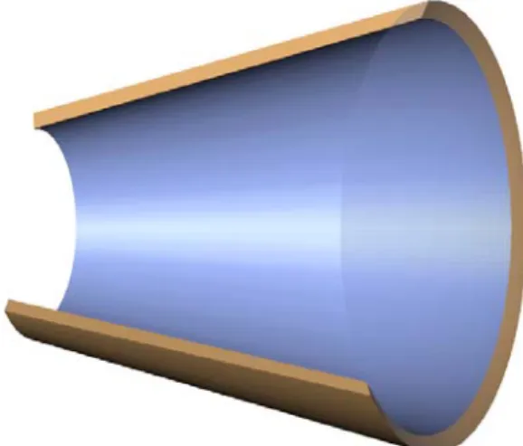
Figure 1-3: Conic nozzle

1.3 Boundary Conditions

In order to deal with open configurations, we consider the boundary to be divided into two regions: the inlet and outlet surfaces, where the fluid crosses the boundary; the nozzle’s walls and the symmetry axis, assumed as flux surfaces.

A simple representation of the problem geometry is the conical nozzle illustrated in fig (1-3). This consists in a conical wall surface delimited by two spherical surfaces in the inlet and outlet region. The example is also a test case for the procedure. In particular, this geometry is easily described by using spherical coordinates (σ, θ, φ), as illustrated in figure (1-4), where the domain can be defined as σ ∈ [σinlet, σoutlet] and θ ∈ [0, θwall].

In the variational formulation we consider the case of fixed boundary conditions where the values of the unknown function ψ is assigned on ∂Ω. In another classic type of boundary con-dition, relevant to the problem of plasma propagation, we seek an extremum of the Lagrangian when the values assumed by ψ on a portion ∂1Ω of the whole boundary ∂Ω are not specified. It

can be shown that, due to the Lagrangian extremum condition, a specific boundary condition must be satisfied on ∂1Ω. In fact, taking the first variation of our functional, we obtain with

(26)

Figure 1-4: Spherical coordinate system used for the description of conic nozzle geometry some manipulations: δL = Z Ω[L]ψ δψdV + Z Ω[L]ρ δρdV + Z Ω[L]vϕ δvϕdV + Z ∂1Ω µ Lψ_z dr ds − Lψr dz ds ¶ δψdS,

where [L]ψ, [L]ρ, [L]vϕ represent the Euler-Lagrange equations associated with the three

vari-ables of our problem. As before, this variation should be zero. It is easy to prove that, since the extremum solution for these boundary conditions is an extremum also for the classic boundary condition, the three volume integrals are zero. Thus, for the arbitrariness of the variations δψ the equation for the boundary ∂1Ω results

∂L (x, vϕ, ρ, ψ, ∇ψ) ∂ (∂ψ/∂r) dz ds − ∂L (x, vϕ, ρ, ψ, ∇ψ) ∂ (∂ψ/∂z) dr ds = 0, (1.47)

where s is the boundary arc-length. This boundary condition is called the natural boundary condition of the problem.

As a consequence of the definition of the flux function ψ, we can now assume the Dirichlet condition on the nozzle’s wall and on the symmetry axis:

ψ|axis= ψ0 ψ|wall= ψ1 (1.48)

whereas in the open parts of the boundary we shall prescribe the natural conditions. The choice of natural boundary conditions fully determines the problem from a mathematical point

(27)

of view and, since these conditions are naturally satisfy by the variational formulation, it permits a simple implementation of the open boundary geometry. However the solution still depends on the shape of the inlet and outlet surfaces and a study of this dependence is recommended in order to characterize the different solutions. In general we should consider the shape related to the plasma properties outside the domain of the nozzle and the analysis of different geometries can contribute to describe these relations. It is easy to see that the difference ψ₁_−ψ₀represents the overall flow rate of the corresponding vector field passing through the domain. Since the flux function ψ is defined except for a constant additional value, it is a common choice to assume ψ₀ = 0. Thus, hereafter ψ represents the net flux enclosed in the axisymmetric surface that it labels.

1.3.1

Substituting the Lagrangian density L in (1.47) and carrying out the calculation, the natural boundary condition can be rewritten in the form:

1 r2

∇ψ

ρ · n = 0. (1.49)

Considering the relation between the mass flow and ψ (1.12), in the part of ∂Ω where we impose no condition on ψ, we are asking for a solution with a poloidal velocity field flowing perpendicularly to the boundary. This assumption is the same as prescribing the tangent component of the crossing fluid velocity in each point of the open-boundaries and from equation (1.49) we obtain: ∇ψ · n|i,o= 0 → ∂ψ ∂n ¯ ¯ ¯ ¯ i,o = ∂ψ ∂σ ¯ ¯ ¯ ¯ i,o = 0, (1.50)

where the indices i and o distinguish respectively the inlet and outlet boundary properties. Integrating the normal flux

ρ_iV_iσ = 1 σ2_{sin (θ)} ∂ψ ∂θ ¯ ¯ ¯ ¯_i along the inlet surface yields

σ2_i Z θ

0

(28)

and for θ = θwall we obtain the diﬀerence between the two boundary values.

From equation (1.51), giving an estimate of ρ_i, pi, Vi and Vφin the inlet region, we obtain

the explicit expressions of A, B and C in terms of stream function ψ. Recalling the definition, we have A (θ)|i = Vφ(θ) · σisin (θ) , (1.52) B (θ)|i = V_i2(θ) 2 + V2 φ(θ) 2 + γ γ − 1 pi(θ) ρ_i(θ), (1.53) C (θ)|i = pi ργ_i , (1.54) while θ|i= θ (ψ) (1.55)

is obtained by inverting equation (1.51).

Given these conditions (1.48-1.50 and 1.52-1.55) the problem is fully formulated and is possibly solvable, provided that a solution exists.

1.3.2

By substituting the Lagrangian density (1.45) into equation (1.47), we obtain the equivalent expression of the natural condition for the MHD problem:

1 r2 µ F2 4πρ− 1 ¶ ∇ψ · n = 0.

In the open parts of the boundary, where we assume the natural condition to hold, this equation yields ∇ψ · n|i,o= 0 → ∂ψ ∂n ¯ ¯ ¯ ¯ i,o = ∂ψ ∂σ ¯ ¯ ¯ ¯ i,o = 0, (1.56)

where the indices i and o distinguish respectively the inlet and outlet boundary. It is easy to see that the diﬀerence ψ₁_{− ψ}₀ represents the overall magnetic induction passing through the domain. In fact, by integrating the normal flux

B_iσ = 1 σ2_{sin (θ)} ∂ψ ∂θ ¯ ¯ ¯ ¯ i

(29)

in the inlet surface, we derive

σ2_i Z θ

0

sin (θ) B_iσdθ = ψ_i_{(θ) − ψ}₀ (1.57)

and for θ = θwall we obtain exactly the diﬀerence between the two boundary values.

From equation (1.57), giving an estimate of ρ_i, pi, Vi, Vφ, Bi, Bφ, in the inlet region, we

deduce the explicit expressions of F , G, H, I and J in terms of stream function ψ. Recalling the definition, we have

F (θ)|i = 4πρi(θ) Vi(θ) Bi(θ) (1.58) G (θ)|i = 1 σisin (θ) ∙ Vφ(θ) − Vi(θ) Bi(θ) Bφ(θ) ¸ , (1.59) H (θ)|i = σisin (θ) ∙ Bφ(θ) − 4πρi(θ) Vφ(θ) Vi(θ) Bi(θ) ¸ (1.60) I (θ)|i = pi(θ) ργ_i (θ) (1.61) J (θ)|i = V_i2(θ) 2 + V2 φ (θ) 2 + γ γ − 1 pi(θ) ρ_i(θ)− Vφ(θ) ∙ Vφ(θ) − Vi(θ) Bi(θ) Bφ(θ) ¸ , (1.62) while θ|i= θ (ψ) (1.63)

is obtained by inverting equation (1.57). The substitution of equation (1.63) into equation. (1.58-1.62) yields the explicit expressions of the five functions of ψ.

1.4 Discontinuous Solutions

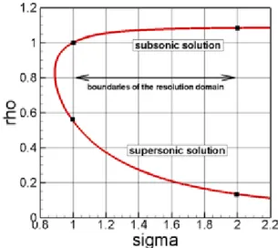
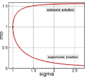
The variational formulation allows us to find the solution in a more general class of functions. This yields a simple method to include the shocks in our analysis. It is well known that hydrodynamic equations are locally elliptic or hyperbolic depending on the ratio between the velocity and the speed of sound (Mach number). We can see that in some cases, for the same mass flow rate, two diﬀerent solutions can be found, one with a subsonic flux and the other with a supersonic one. If we relax the hypothesis of isentropic flow considering that somewhere in the domain the entropy function passes from S to S + ∆S, it is possible to determine a

(30)

new solution with both subsonic and supersonic regimes. This solution and the position of the entropy’s transition surface depend on the chosen value of the entropy jump ∆S. For the physically meaningful cases (∆S > 0) the transition is from a supersonic flow to a subsonic one and is called a "shock " because the fluid properties change discontinuously through it.

An important feature of the variational principle (1.36) is that the solution of the general problem of hydrodynamic and magnetohydrodynamic flow with shocks can be implicitly car-ried out assuming that the derivatives of the flux function ψ and the density ρ are piecewise continuous.

Let us assume that a discontinuity surface λ (a curve in the poloidal plane) exists which divides the domain into two parts: Ω1and Ω2. Thus, given a general function χ (x, y), we define

as

kχk = χλ2− χ_λ1 (1.64)

the diﬀerence between the two limits

χ_λ2 = lim

x→λχ x ∈ Ω2,

χ_λ1 = lim

x→λχ x ∈ Ω1

at a generic point of λ.

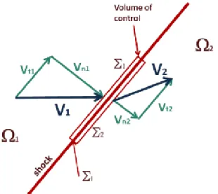
Consider a frame of reference locally aligned with the discontinuity surface. In this frame the velocity and the magnetic induction vectors can be written as

V= vnn+ vtt+ vφφ,

B= Bnn+ Btt+ Bφφ,

where n and t represent respectively the normal and the tangential unit vector to λ in the symmetry plane.

A first way to determine the jump conditions across the discontinuity is to use the integral form of the model’s equations (1.1)-(1.7). Consider an infinitesimal cylindrical volume element, illustrated in figure (1-5), where the bases of the cylinder are parallel to the shock surface and the bases’ typical dimension is bigger than the distance between them. The mass conservation

(31)

Figure 1-5: Schematic description of a shock transition

equation (1.1), which is the same for the two models we are investigating, in its integral form can be written as Z Σ1 ρ₁V1·n1dS1+ Z Σl (ρV · n)|ΣldSl+ Z Σ2 ρ₂V2·n2dS2 = 0,

where the flux term through the surface Σl can be neglected, for h ¿ r, thus obtaining

Z Σ1 ρ₁V1·n1dS1+ Z Σ2 ρ₂V2·n2dS2= 0.

This expression can be rewritten, by using the definition (1.64), as

kρvnk = 0. (1.65)

These same considerations hold for the remaining model’s equations (1.2)-(1.7) but specific care must be taken for energy conservation. Our attempt is to model entropy discontinuity in an

(32)

adiabatic flow. Thus, instead of equation (1.3), we shall use the energy equation Z (ρV · n) µ e + V 2 2 ¶ dS + Z pn · VdS + Z _c 4πE× B · ndS = 0. (1.66)

In this way we obtain a number of jump constraints equal to the number of conservation equations.

The same constraints can be found through the extremization of the Lagrangian functional (1.43) on the set of functions

U ≡©¯ρ piecewise continuous, ¯_{ψ ∈ C}0 _{: ∇¯}ψ piecewise continuousª (1.67) Hence equation (1.43) can be written as:

L(ρ, ψ) = Z Ω1 L1(x, ρ, ψ, ∇ψ) dV + Z Ω2 L2(x, ρ, ψ, ∇ψ) dV (1.68)

where the only diﬀerence between L1 and L2 is in the entropy term. Let us suppose that two functions {ρ, ψ} ∈ U give an extremum of the functional (1.68). By assuming that the discontinuity surface λ is fixed according to the solution’s one, if we search for an extremum in the subset U it obviously follows that the solution will be the same as in the general case (no fixed λ). However, since this problem is equivalent to the traditional one, we can conclude that in the two sub-domains the solution satisfies the classical Euler-Lagrange equations associated with the Lagrangian principle.

Considering a double integral of a general function u = u (x, y)

J = ZZ

Ω

F (x, y, u, ux, uy) dxdy, (1.69)

the first variation became:

δJ = Z ∂Ω µ Fux dy ds − Fuy dx ds ¶ δu · ds + ZZ Ω [F ] dxdy.

(33)

domain, we can write the first term on the right side in the form Z ∂Ω ¡ Fuxnx+ Fuyny ¢ δu · ds. (1.70)

Now, using the expression (1.64) for the integral (1.70), it follows that

δJ = Z λ ¡ kFuxk nx+ ° °Fuy ° ° ny ¢ δu · ds = 0,

where n is the normal vector on λ, pointing outside the domain Ω1. For the arbitrariness of δu,

we conclude that kFuxk nx+ ° °Fuy ° ° ny = 0, (1.71)

for each point on λ.

In the derivation of this condition we have assumed that λ is fixed. If we take the variation induced by the arbitrariness of the shock surface we obtain one more condition in the form

kF k = Fux|1kuxk + Fuy

¯ ¯

1kuyk , (1.72)

where the index 1 means that the expression is evaluated on the Ω1 side (details on this

deriva-tion can be found in Smirnov [34]).

So, the problem can be equivalently solved using the diﬀerential approach, with the bound-ary conditions and the shock conditions like (1.65), or finding an extremum of the Lagrangian principle with the condition (1.67). From a numerical point of view it is thus possible to model the hydrodynamic and magnetohydrodynamic flows with shock surfaces within the variational theory by including the position of the shock among the unknowns.

1.4.1

In the hydrodynamic case the equations necessary to obtain the jump condition across a dis-continuity of the flux entropy are the mass conservation equation, previously described, the momentum and the energy conservation equations. The integral formulation of the momentum

(34)

balance can be written as

I

(ρV · n) VdS + I

pndS = 0, while the energy conservation yields

I (ρV · n) µ e + V 2 2 ¶ dS + I pn · VdS = 0,

where e (x) represents the specific internal energy of the fluid. By exploiting the notation introduced before, due to the arbitrariness of the integration surfaces we obtain, from the first equation,

kρvnV+ pnk = 0, (1.73)

and, from the second equation, ° ° ° °ρvn µ e +V 2 2 ¶ + pvn ° ° ° ° = 0. (1.74)

The condition (1.65) can now be used to simplify the term ρvn in the above equations.

Even-tually we have the following system of equations that describes univocally the discontinuous changes of the flow properties

kρvnk = 0, (1.75a) ° °ρv2 n+ p ° ° = 0, (1.75b) kvtk = 0, (1.75c) kvφk = 0, (1.75d) ° ° ° ° V2 2 + h ° ° ° ° = 0, (1.75e)

where h = p_ρ + e represents the specific fluid’s enthalpy. The arrangement of the conditions (1.75), called the Rankine-Hugoniot’s conditions, yields the well-known shock equation

ρ₂ ρ₁ = (γ + 1) M₁2 2 + (γ − 1) M12 , (1.76) where M1 = q ρ1v12

(35)

From the foregoing, a diﬀerent way to determine the Rankine-Hugoniot conditions is by exploiting the variational principle of the model. The continuity of the stream functions still holds and yields to equations (1.75d) and (1.75e)

kvφk = ° ° ° ° A (ψ) r ° ° ° ° = 0, ° ° ° ° V2 2 + h ° ° ° ° = kB (ψ)k = 0. By using the definition of ψ, equation (1.12), we obtain

kρvnk =

1

r k∇ψ · tk = 0,

where the last equality can be deduced from the continuity properties of the stream function in the direction tangential to the shock. This directly implies the condition (1.75a).

Two conditions remain that can be derived from the equations (1.71) and (1.72), in the hypothesis of a discontinuous adiabatic flow. In fact, substituting the expression (1.42), equation

(1.71) yields _° ° ° ° 1 r2 ∇ψ ρ ° ° ° ° · n = 0 (1.77)

that represent the tangential velocity conservation across the shock surface, equation (1.75c). Due to expression (1.42), the equation (1.72) reduces to

|L| = _r12_ρ ∂ψ ∂z ¯ ¯ ¯ ¯ 1 ° ° ° °∂ψ_∂z ° ° ° ° + _r12_ρ ∂ψ ∂r ¯ ¯ ¯ ¯ 1 ° ° ° °∂ψ_∂r ° ° ° ° (1.78)

Combining this jump condition with equation (1.77) and with the continuity of the flux function ψ through the shock yields the requested equation (1.76) (the details are worked out in Appendix A).

1.4.2

Following the arguments of the hydrodynamic model, we now describe the changes in the jump condition for MHD flows with shock transitions. In the momentum and energy equations are

(36)

added terms related to the magnetic field, I (ρV · n) VdS + I pndS + I _B2 8πndS − I µ _B 4π · n ¶ BdS = 0, (1.79) I (ρV · n) µ e + V 2 2 ¶ dS + I pn · VdS + I _c 4πE× B · ndS = 0. (1.80)

Moreover new conditions arise from Maxwell equations (1.5) - (1.7). The equation (1.79) yields

° ° ° °ρvnV+ pn+ B2 8πn− Bn 4πB ° ° ° ° = 0, (1.81)

which expresses shows the conservation of momentum in the three components, normal to the

discontinuity surface _° ° ° °p + ρvn2+ B2 8π − B_n2 4π ° ° ° ° = 0, (1.82)

and in the tangent plane ° ° ° °ρvnvt− BnBt 4π ° ° ° ° = 0, ° ° ° °ρvnvφ− BnBφ 4π ° ° ° ° = 0. (1.83)

The analogy between the Lagrangian density and the equation (1.82) shows a possible meaning of the variational principle: the solution is an extremum of the total momentum in the flow direction.

From the energy equation it follows that ° ° ° °ρvn µ e + V 2 2 ¶ + pvn+ B2 4πvn− (v · B) Bn 4π ° ° ° ° = 0,

that can be further manipulated using the definition of specific enthalpy and the mass flow

condition (1.65) as _° ° ° °h + V2 2 + B2 4πρ− (v · B) Bn 4πρvn ° ° ° ° = 0. (1.84)

The Maxwell equations for the magnetic induction yield three more condition. From the divergence equation we obtain

(37)

and from Faraday’s equation n_{× kEk = n×} ° ° ° ° v_{× B} c ° ° ° ° = 0, (1.86)

where the second equality derived from the perfect conductivity equation. This last vectorial condition can be expressed in terms of each single component, in the reference system defined by the discontinuity position. It is easily shown that the component parallel to the normal unit vector is nothing. In the azimuthal direction the equation (1.86) becomes

k−vnBφ+ vφBnk = 0,

and the other component tangent to the shock results

kvnBt− vtBnk = 0.

The system of conditions formed by the equations (1.65), (1.81), (1.85), (1.86) defines the jump conditions for a plasma flow through an entropy discontinuity. Like the hydrodynamic case, this system can be derived from the variational formulation of the problem. The continuity of the stream function ψ yields

kBnk =

1

rk∇ψ · tk = 0 (1.87)

and the four functions that depend on ψ give four more of the jump condition,

kF (ψ)k = ° ° ° °4π ρvn Bn ° ° ° ° = kρvnk = 0, kG (ψ)k = ° ° ° ° 1 r µ vφ− vnBφ Bn ¶°°_° ° = k−vnBφ+ vφBnk = 0, kH (ψ)k = ° ° ° °4πrρv_B_nnvφ− rBφ ° ° ° ° = ° ° ° °ρvnvφ− BnBφ 4π ° ° ° ° = 0, kJ (ψ)k = ° ° ° °h + V2 2 + B2 4πρ− (v · B) Bn 4πρvn ° ° ° ° = 0, where equation (1.87) has been used to simplify the term Bn.

(38)

By assuming the discontinuity of the plasma density ρ and of the gradient of ψ in the direction normal to the shocks, two more conditions follow. In fact, substituting the expression (1.45) in (1.71) we obtain _° ° ° ° 1 r2 µ F2 4πρ− 1 ¶ ∇ψ ° ° ° ° · n = 0, (1.88)

that represent the tangential momentum conservation across the shock surface, equation (1.83). Due to expression (1.45), the equation (1.72) reduces to

|L| = µ F2 4πρ− 1 ¶ 1 ∙ 1 4πr2 ∂ψ ∂z ¯ ¯ ¯ ¯₁ ° ° ° ° ∂ψ ∂z ° ° ° ° + 1 4πr2 ∂ψ ∂r ¯ ¯ ¯ ¯₁ ° ° ° ° ∂ψ ∂r ° ° ° ° ¸ . (1.89)

Combining this jump condition with equations (1.88)-(1.89) yields the required remaining equa-tion.

(39)

Chapter 2 Numerical Procedure

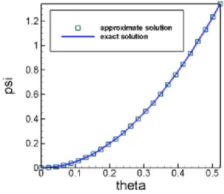
After the discussion of the theoretical model, we apply a numerical procedure that permits a complete description of fluid and plasma flow and the achievement of a reasonable under-standing of the acceleration processes. The variational approach has a fundamental role in our attempts. This permits the use of a simple approximation method, the Ritz method. By scal-ing the Lagrangian functional it is first possible to render all the equations dimensionless. The extremum is confined in a finite-dimensional functions subspace and the solution is obtained through a system of non-linear equations. This system is solved by using the Newton-Raphson algorithm. A simple semi-analytic solution is finally presented to be utilized as a validation test of the procedure.

2.1 Non-Dimensionalization

In order to obtain a dimensionless model we start scaling the Lagrangian density variables with typical values, values of the size we expect to see or dictated by the geometry. Instead of a large number of physical parameters and variables, all with dimensional units, we are left with equations written in dimensionless variables. All the physical parameters and typical values are collected together into a smaller number of dimensionless parameters (or dimensionless groups) which, when suitably interpreted, should tell us the relative importance of the various mechanisms.

Another advantage of the scaling is the improvement in the numerical precision. This is because the numerical operations are carried out between numbers of the order of the unity.

(40)

All of this is much easier to see by working through an example, so we start directly with the hydrodynamic model where we can see the advantages of this technique.

2.1.1

Axisymmetric Hydrodynamics

In both the hydrodynamic and magnetohydrodynamic cases, the natural candidate for the length scale is the inlet spherical radius r0 = σin of the conical nozzle. Then, for a

non-conductive fluid we can scale the fluid density and velocity with the inlet typical values ρ₀ and V0 and the flux function with ψ0 = r20ρ0V0. Since the azimuthal behavior is governed by a

diﬀerent equation we shall use a diﬀerent value for the scaling of vφ. We introduce the value

V0φ, again related to the inlet condition, and consequently A0 results

A0= V0φr0. (2.1)

The remaining stream functions can be scaled in diﬀerent ways but here we adopt these typical values B0 = V2 0 2 , (2.2) C0= p0 ργ₀, (2.3)

where p0 is the reference value for the fluid pressure.

Rewriting the Lagrangian density (1.42) in dimensionless units, hereafter designated by the hat sign (e.g. ˆa), we obtain

L³ˆx, ˆρ, ˆψ, ˆ_∇ˆψ´= 1 2ρ0 µ ψ₀ ρ₀r2 0 ¶2 ˆ ρ Ã 1 ˆ r ˆ ∇ˆψ ˆ ρ !2 − 1 2ρ0 µ A0 r0 ¶2 ˆ ρ " ˆ A ˆ r #2 + ρ₀B0ˆρ ˆB − 1 γ − 1ρ γ 0C0ˆρ γ_C._ˆ

The dimensionless gradient can be expressed as:

∇ = _r1

0

ˆ ∇.

(41)

as expressed in spherical coordinates ∇ = eσ ∂ ∂σ+ eθ 1 σ ∂ ∂θ. Then we resize the coordinates to obtain a unit square domain:

ˆ ∇ = ex 1 hx ∂ ∂x+ ey 1 hy ∂ ∂y,

where the elements hx,y defines the new metric adopted. The following equations hold

∂ ∂σ = 1 ∆σ ∂ ∂y 1 σ ∂ ∂θ = 1 θwall µ 1 σin+ ∆σs ¶ ∂ ∂x. These last expressions can be simplified by putting

Xdim = θwall, Ydim=

∆σ σin , (2.4) which imply hx = Xdim(1 + Ydim· y) , hy = Ydim.

From equations (2.2-2.3) it follows that L 1 2ρ0V02 = ρ µ 1 r ∇ψ ρ ¶2 − R20ρ ∙ A r ¸2 + ρB − 2M −2 0 (γ − 1) γρ γ_C, _(2.5)

where the hats have been dropped and we have introduced the two dimensionless numbers

M0 = V0 a0 = _qV0 γp0 ρ₀ Mach number, (2.6) R0 = V0φ V0

Azimuthal velocity ratio. (2.7)

The problem resolution now depends only on the two geometrical factors (2.4) and the two dimensionless numbers (2.6-2.7) in order to characterize diﬀerent solutions.

(42)

2.1.2

As for the hydrodynamic case, a general simplification for the numerical solution and for the results analysis is obtained through the non-dimensionalization of the model equations. We can begin scaling all the variables with typical values and rewriting the Lagrangian density (1.45)

L = µ ψ₀ r2 0 ¶2Ã F₀2 4πρ₀ ˆ F2 ˆ ρ − 1 ! 1 8π Ã ˆ ∇ˆψ ˆ r !2 + 1 8πr2 0 Ã H0H + rˆ 0V0φF0rˆˆvφFˆ r !2 − 1 2ρ0 ³ V₀φ´2ˆρˆv_φ2+ ρ₀ˆρ³J0J + rˆ 0V0φG0ˆrˆvφGˆ ´ − 1 γ − 1ρ γ 0I0ˆργIˆ (2.8)

In this expression we have again denoted the dimensionless quantities by the hat sign ‘ˆa’ and the characteristic scale-lengths by the subscript zero ‘a0’. The length scale is the inlet spherical

radius r0 = σin of the conical nozzle, B0 is the typical value of the magnetic field and we can

scale the flux function with ψ₀ = r2

0B0. The dimensionless gradient can be expressed as

∇ = _r1

0

ˆ ∇

where the definition of ˆ_{∇ and the two geometrical parameters (X}dim, Ydim) are the same defined

in the previous subsection.

Then we take some more assumptions on the non-dimensional quantities and we scale F...J respectively with F0 = 4πρ_B0V₀0, G0 = _2rV0₀, H0= r0B0, I0= _ρp0γ 0, J0 = V 2 0 2 .

By using these definitions it follows that L 1 8π ³_ψ 0 r2 0 ´2 = µ M₁2F 2 ρ − 1 ¶ µ ∇ψ r ¶2 + µ H + M1M2rvφF r ¶2 − ... (2.9) −M22ρv2φ+ M12ρJ + M1M2rρvφG − M2 1 M2 0 2 (γ − 1) γρ γ_I,

(43)

where the hats have been dropped and we have introduced the three dimensionless numbers M0 = V0 a0 = qV0 γp0 ρ0 Mach number, (2.10) M1 = V0 VA0 = s F₀2 4πρ₀ Mach-Alfven number, (2.11) M2 = V0φ VA0 = s 4πρ₀V2 0φ

B₀2 Mach-Alfven azimuthal number. (2.12)

We are left with an equation written in dimensionless variables and all the physical parameters and typical values are collected together into a smaller number of dimensionless parameters. Again the solution depends on the two geometrical factors (2.4) and on the three dimensionless numbers (2.10-2.12).

2.2 The Ritz Method

In giving an existence proof for a solution to a variational problem one requires the existence of minimizing sequences, with suitable convergence and functional properties. In practical applications there still remains the problem of actually constructing a minimizing sequence, and, furthermore, one which converges with a fair degree of rapidity. The method described below was first introduced by W. Ritz [27][28], who applied it to problems concerning elastic plates.

We consider a variational integral I (Φ) defined over a compact set R of admissible functions. A numerable sequence of functions w1, . . . , wn contained in the class R is said to be complete

if every function Φ in R can be approximated by a finite linear combination Wn= a1w1+ a2w2+ . . . + anwn

(44)

can be understood in several senses. Given any Φ in R and any ε, we want a Wn such that (a) _{|I (Φ) − I (W}n)| < ε, (b) Z Ω(Φ − W n)2dx < ε, (c) _{|Φ − W}n| < ε.

In the following we shall take the approximation in the sense (a).

For example, we know from the theory of Fourier series that the sequence of functions

sin (nπx) (n = 1, 2, . . .)

forms a complete system for all functions Φ (x) which are continuous, have a piecewise contin-uous derivative, and vanish at 0 and 1.

Except for the trigonometric functions, the most important and most useful complete system is given by the integer powers of x, or, in two dimensions, xnym. The linear combination of such functions are polynomials. Weierstrass proved the following important theorem:

If f (x) is an arbitrary continuous function in a closed interval, then it may be approximated in this interval to any desired degree of accuracy by a polynomial Pn(x), provided that n is

taken suﬃciently large. This theorem is valid for higher dimensions as well.

Returning to the given variational integral I (Φ), we suppose, in order that the problem make sense, that the integral has a greatest lower bound d. It immediately follows the existence of minimizing sequences Φn such that I (Φn) → d. The Ritz method consists in replacing the

minimizing sequence by means of a sequence of auxiliary minimum problems. We consider, for a fixed n, the integral

I (Wn) = I (a1w1+ a2w2+ . . . + anwn) ,

where w1, . . . , wnare the first n numbers of a complete system {wn} of the admissible functions

of the set R. Then, the integral becomes a function of the n coeﬃcients a1, . . . , an varying

independently. We next consider the problem of finding the set of coeﬃcients a1, . . . , an which

(45)

parameters a1, . . . , an, it must attain a minimum; according to the ordinary theory of maxima

and minima, the system of n equations ∂ ∂ai

I (Wn) = 0

permits to determine the particular values ai = ci which give the minimum. We denote the

minimizing function by un = c1w1 + . . . + cnwn. The essence of the Ritz method is then

contained in the following theorem:

The sequence of functions u1, . . . , un, which are the solutions to the successive minimum

problems I (Wn) formed for each n, are a minimizing sequence to the original variational

prob-lem.

First, it is seen that I (un) is a monotonically decreasing function of n, since we may regard

every function W_n−1 _{admissible in the (n − 1)}th minimum problem as an admissible function for the nth minimum problem with the additional side condition an= 0. Therefore

I (un) → δ ≥ d.

Next, the existence of a minimizing sequence {Φn} to the variational problem implies that,

for some suﬃciently large k,

I (Φk) < d +

ε 2.

Since the system w1, . . . , wnis complete, there exists a suitable function Wn= a1w1+. . .+anwn

such that I (Wn) < I (Φk) + ε 2. But, by definition of un, I (un) ≤ I (Wn) , hence I (un) < d + ε,

which establishes the convergence of I (un) to d.

(46)

of n equations:

∂ ∂ai

I (Wn) = 0.

The process is considerably simplified if the given functional is quadratic, since in that case we have a system of linear equations in the a’s.

As an example of the Ritz method, let us consider the case where on the boundary Φ = g is a polynomial, the boundary being given by B (x, y) = 0. If we take for functions Φ the functions

Φ = g + B (x, y) (a + bx + cy + . . .) ,

this sequence of functions Φ is a minimizing sequence, and I (Φ) is a function I (a, b, c, . . .) of the coeﬃcients a, b, c, . . ., and the problem is reduced to finding the minimum of I with respect to a, b, c, . . ..

2.2.1

Axisymmetric Hydrodynamics

By exploiting the Rayleigh-Ritz Method, we search for a simple approximation of ψ and ρ through the extremization of the functional (1.42). We start assuming that the approximation functions belong to a finite dimensional subspace of the solution space, thus considering ψ and ρ sums of base-function. These can be written in the form

ψ (x, y) = nT X n=0 ψ_nFn(x, y) = ni X i=0 nj X j=0 ψ_ijF_ix(x) F_jy(y) , (2.13) ρ (x, y) = mT X m=0 ρ_mGm(x, y) = mi X i=0 mj X j=0 ρ_ijGx_i (x) Gy_j(y) , (2.14)

where Fx,y and Gx,y are two families of base-functions. The two series are truncated and nT

and mT are the numbers of functions used. Some common choices are:

F_ix,y(t) , Gx,y_i (t) ⎧ ⎪ ⎪ ⎪ ⎨ ⎪ ⎪ ⎪ ⎩ ti cos (it) . . . .

(47)

It is usually preferred to approximate the solution with smooth functions, choosing the base that best represents the solution as we suppose it will be. It is also important to avoid singularities in the integrals of these functions. Substitution of this expression into (1.36) implies

L¡ψ₁, ...ψ_n_T, ρ₁, ..., ρ_m_T¢= Z

ΩL (x, ρ (ρm

) , ψ (ψ_n_{) , ∇ψ (ψ}_n)) dV, (2.15)

and the extremization process can be developed diﬀerentiating (2.15) with respect to ψ_n and ρ_m ∂L ∂ψ_n = Z Ω ∂L ∂ψ_ndV ∂L ∂ρ_m = Z Ω ∂L ∂ρ_mdV. From (2.5) we have ∂L ∂ψ_n = Pn ¡ ψ₁, ...ψ_n_T, ρ₁, ..., ρ_m_T¢, (2.16) where Pn ¡

ψ₁, ...ψ_n_T, ρ₁, ..., ρ_m_T¢has the expression

Pn= 2 r2 ∇ψ ρ · ∇fn+ ρ " −2R20 A ˙A r2 + ˙B − 2M₀−2 (γ − 1) γρ γ−1_C˙ # · fn, and ∂L ∂ρ_m = Rm ¡ ψ₁, ...ψ_n_T, ρ₁, ..., ρ_m_T¢, (2.17) with Rm¡ψ1, ...ψnT, ρ1, ..., ρmT ¢ given by Rm= " − µ 1 r ∇ψ ρ ¶2 − R02 µ A r ¶2 + B − 2M −2 0 (γ − 1)ρ γ−1_C # · gm.

Hence the approximation coeﬃcients are a solution of the non-linear system of equations h

P1 · · · PnT R1 · · · RmT

i

= 0. (2.18)

Observe that in the incompressible case the problem can be linear if the condition A ∝ ψ and B ∝ ψ2 hold.

(48)

2.2.2

Again we start assuming that the approximation functions belong to a finite dimensional sub-space of the solution sub-space. Considering the expansion of ψ, ρ and vφas sums of base-functions,

the three unknown functions can be written in the form:

ψ (x, y) = nT X n=0 ψ_nFn(x, y) = ni X i=0 nj X j=0 ψ_ijF_ix(x) F_jy(y) , (2.19) ρ (x, y) = mT X m=0 ρ_mGm(x, y) = mi X i=0 mj X j=0 ρ_ijGx_i (x) Gy_j(y) , (2.20) vφ(x, y) = lT X l=0 vφlHl(x, y) = li X i=0 lj X j=0 vφijHix(x) H y j (y) , (2.21)

where Fx,y, Gx,y and Hx,y are three families of base-functions and nT, mT and lT are the

number of functions used.

Following the same arguments as before, we obtain

L = Z

ΩL (x, v

φ(vφl) , ρ (ρm) , ψ (ψn) , ∇ψ (ψn)) dV, (2.22)

and the extremization process can be developed diﬀerentiating (2.15) with respect to three sets of coeﬃcients {ψn, ρm, vφl} ∂L ∂ψ_n = Z Ω ∂L ∂ψ_ndV ∂L ∂ρ_m = Z Ω ∂L ∂ρ_mdV ∂L ∂vφl = Z Ω ∂L ∂vφl dV.

The arguments of the integrals, deduced from the dimensionless expression (2.9) of the La-grangian density, result:

∂L ∂ψ_n = Pn ¡ ψ₁, . . . , ψ_n_T, ρ₁, . . . , ρ_m_T, vφ1, . . . , vφlT ¢ , (2.23)

A variational treatment of hydrodynamic and magnetohydrodynamic flows