1
Supporting Information
Failure Processes in Embedded Monolayer Graphene under Axial Compression
Charalampos Androulidakis, Emmanuel N. Koukaras, Otakar Frank, Georgia Tsoukleri, Dimitris Sfyris, John Parthenios, Nicola Pugno, Konstantinos Papagelis, Kostya S. Novoselov, and Costas Galiotis*
1. Mathematical Analysis
According to the Euler stability criterion, the critical state for compression failure is reached
when the work of the external forces equals the change in strain energy of the body1,2:
(S1)
Furthermore, the work of the compressive forces acting on the middle plane of the plate is
given by2:
(S2)
where u is the out-of-plane displacement, A is the area of the plate (graphene) and Nx is the
compressive force along the x-direction. The bending energy is given by2:
2 2 2 2 2 2 2 2 2 2 1 2 2 , 2 b A D u u u u u U v dA x y x y x y
(S3)where D is the bending stiffness and v the Poisson ratio of graphene. The surrounding
polymer matrix is assumed to contribute to the system through the deformation energy:
, b f. T U U U U 2 1 , 2A x u T N dA x
2 (S4)
where Kw is the Winkler’s modulus. From the physical point of view the last term describes
the interaction between the plate and the elastic foundation which is loaded as the plate bends
at the critical point.
By equating the work of the external forces with the change in the strain energy we
obtain:
2 2 2 2 2 2 2 2 2 2 2 2 2 1 2 2 1 . 2 2 b W x A w A A T U U u N dA x K D u u u u u v dA u dA x y x y x y
(S5)For the out-of-plane displacement it is common to assume that it has a sinusoidal form2-6
which models adequately the form of buckling that appears at the critical strain. For our
purposes we make the following assumption for u:
1 1 , mnsin sin , m n m x n y u x y a l w
(S6)where l, w is the length and the width of the flake, respectively. Under the above assumption
we obtain: 2 , 2 w f A K U u dA
3 (S7)
(S8)
(S9)
Using the expression on eq 5 we obtain the critical force Nx:
(S10)
Following the reasoning similar to reference 2, the critical force Nx, being a sum of positive
quantities, is minimized when only one term αmn is different than zero. In such a case we
have:
(S11)
If we further make the physically plausible assumption2 that there are several half waves in
the direction of compression but only one half wave in the perpendicular direction (n=1) and
use the formula Nx=εC, where C is the tension rigidity, we finally arrive at the following
expression for the critical strain for buckling: 2 4 2 2 2 2 2 1 1 , 8 b mn m n lw m n U D a l w
2 2 2 1 1 , 8 xxm mn w T N m a l
2 1 1 . 8 w f mn m n K lw U a
2 4 2 2 2 2 2 2 1 1 1 1 2 2 2 1 1 8 8 . 8 w mn mn m n m n x xx mn m K lw lw m n D a a l w N w N m a l
2 2 2 2 2 2 2 2 2 2 2. w x l K l D m n N m l w m 4 (S12)
where
(S13)
The determination of the half waves, m, stem from equating the force expression 11, for m
and m+1:
(S14)
This way we obtain the following equation for m:
(S15)
The evaluation of the half wavelength and the amplitude relies on the inextensibility
assumption. We assume that for small values of applied strain, the length of the specimen
remains the same after buckling initiates. The wavelength that corresponds to the half-wave
number is evaluated according to the formula:
(S16)
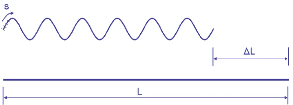
The projection of the buckled length divided by the number of half waves, m, corresponds to
the wave length. The length of the projection can be calculated by: , figure S1 where
. 2 2 2 2 2 , w cr k D k l C w C m 2 . mw l k l mw 1 m m N N 4 4 2 2 4 4 ( 1) l l Kw m m w D
1 cr
l m (l l) cr l l 5
The incompressibility constraint is a plausible assumption since we are at the regime of low
strains (approximately ~-0.5 %). The line integral:
(S17)
corresponds to the length of the flake. In the above relation u is the out-of-plane displacement
that now takes the form:
(S18)
A its amplitude, while the term (1-εcr) describes the contractions due to buckling as the figures shows.
Figure S1. The initial length of the specimen and the length after buckling occurs.
2. Stress transfer from the PMMA to the graphene flake
We apply a compressive loading to the system graphene–PMMA. This kind of loading results
to a shear stress at the interface between the graphene flake and the surrounding medium
which is responsible for transferring the stress to the inclusion (graphene)8. The shear stresses
require a specific length to reach the maximum value of the stress that is possible to be
transferred from the polymer to the graphene. This is the transfer length Lt. So, if the length of
the graphene is smaller than the critical transfer length, Lc (Lc=2Lt) then graphene is not
stressed to the maximum value which is the externally applied stress through the flexure of
PMMA beams. Indeed, only a fraction of the load is transferred to graphene. 2 1 0.5 2 2 1 0 du π π x 1 d 1 cos d d (1 ) (1 ) cr x l x cr cr Am m s x x x l l
max 1 , sin sin , m m m x y u x y A l w
6 Figure S2. Building of stress transfer in graphene.
In the case of flakes with lengths not large enough compared to the required critical length
(Lc), the strain/ stress that is transferred to the flake will never reach the maximum value
(applied strain). Thus, the actual strain developed in the graphene must be corrected as it is
not the same with the external strain. Our experimental results indicate that the flakes with length of up to about ~4 μm are not able to obtain the maximum values of the stresses applied to the system. This is observed by the slope of the curve Pos2D vs Strain (here the strain is
that applied to the beam). In all these cases the slope is much smaller than the critical slope,
~60 cm-1/% (estimate based on the present work as well as values from the literature, see Refs
[9–11]). Thus, a simple correction can be implemented by shifting the Pos2D vs Strain slope
near the origin (zero strain) and recalibrating the actual strain through the formula:
(S20)
3. Fitting
In figure 2 the fourth order polynomial Pos2D=2596 – 56.41ε– 29.54ε2 + 13.16ε3 + 4.01ε4 is
fitted to the data, is in closed form and captures the observed trend of the experimental data
within the full range of strain levels under study. This was the lowest polynomial order that , 0 max , 0 (%) or (%) 60 applied measured
graphene applied graphene
measured imum T
7
yielded acceptable fitting of the data points at both the region near the origin and the region
near failure point. An alternative approach would be to use two separate 2nd degree
polynomials, one for each region of interest. Such polynomials, for example, would have the
form y=2595.8 – 56.1x – 33.2x2 and y=2595.4 – 61.2x – 42.8x2 for the regions near the origin
and at the failure point, respectively. These functions reproduce almost exactly our values for
the slope at the origin and critical strain of failure.
4. Graphene–PMMA Interaction Potentials
Optimized structures
The optimized structures are shown in figure 7 of the manuscript. The structures have a helical pitch of 19.4 Å and 6.75 Å, an outer diameter of 10.1 Å and 23.2 Å, and a helical tilt angle (with respect to the axis of the main chain) of 28.6° and 78.7°, for the i-PMMA and s-PMMA chains respectively. The inner diameter of the s-s-PMMA helix is 13.8 Å which is
substantially larger than the outer diameter of the i-PMMA helix and thus permits the
formation of the 2:1 (s:i) PMMA stereocomplex. These values are in good agreement with the
high-resolution atomic force microscopy measurements on the 2:1 (s:i) PMMA stereocomplex
of Kumaki et al. who reported an outer s-PMMA helix tilt angle of 74°, a chain–chain lateral spacing of 24 Å and a helical pitch of 9.2 Å. Any difference from our theoretical values can be attributed to the influence of the internal i-PMMA double helix of the experimental
stereocomplex structure.
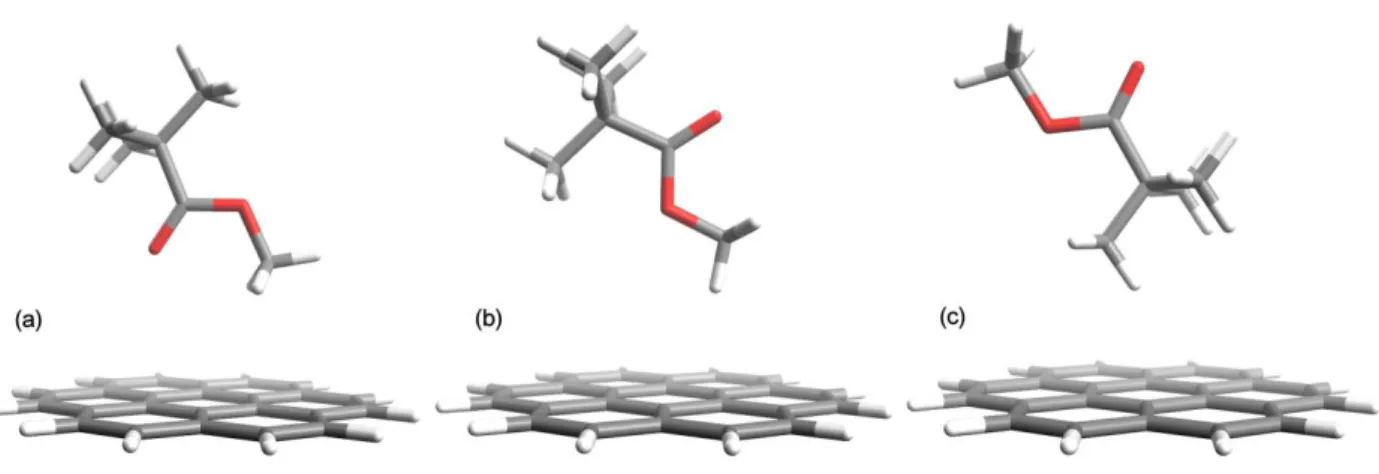
The orientations of the monomers in the optimized polymer chains have been employed as a
guide in selecting the most probable MMA monomer–coronene relative configurations for the
PES scan, which are shown in figure S3. We denote these relative configurations of a MMA
monomer and coronene as h-PC, in which the O–C (single) bond of a MMA monomer is
8
bond of the MMA monomer is vertical, i.e. perpendicular to the coronene plane. The third
configuration corresponds to an approximate reversed h-PC. A fourth configuration, not
shown, corresponds to an h-PC with the monomer’s backbone tilted by 30° with respect to the
normal axis of the coronene plane.
Figure S3. PMMA–coronene relative configurations used for the PES scans. The
configurations correspond to the potentials (a) u1, (b) u2, and (c) u3. A fourth configuration
used is the same as (a) tilted by 30 degrees.
Primitive potentials
Compared to both the results from using the B2PLYPD functional as well as the
SCS(MI)-MP2 method, the B97-D functional slightly overestimates the interaction energy (see figure
S4a). A scaling factor of 1.11 is applied to the values obtained from the B97-D functional in
order to match the results of the more accurate (but impractical for computational reasons)
B2PLYPD functional and SCS(MI)-MP2 method. The primitive potentials are fitted to the
scaled B97-D datasets. The values for the fitting parameters, σ, ε and C, for the primitive
potentials, u1–4, are, ε1 = 18.98 kJmol-1, σ1 = 2.80778 Å, C1 = 0.74371, ε2 = 16.68 kJmol-1, σ2 =
2.99278 Å, C2 = 0.68142, ε3 = 21.59 kJmol-1, σ3 = 2.7788 Å, C3 = 0.68782, and ε4 = 19.09
9 (a) (b) 12 0.74 6 0.74 1 2.81 2.81 ( ) 4 18.98 : 1 u z PES z z 12 0.68 6 0.68 2 2.99 2.99 ( ) 4 16.68 : 2 u z PES z z 12 0.69 6 0.69 3 2.78 2.78 ( ) 4 21.59 : 3 u z PES z z 12 0.79 6 0.79 4 2.91 2.91 ( ) 4 19.09 : 4 u z PES z z
10 (c)
(d)
Figure S4. Potential energy surface scans for the configurations PMMA–Coronene shown in
figure S3. R is the transverse distance of the PMMA carbon atom nearest to the coronene
plane.
Two-parameter PES scan
We have additionally performed a two-parameter PES scan on a coronene with two MMA
molecules, one on each of the coronene surfaces. The configuration corresponds to that used
in PES1, and the scanning parameters are the distances R1, R2 between each monomer and the
11
molecule reduces the interaction very slightly, and the overall interaction energy is 1.2 % less
compared to twice the interaction energy of the corresponding single monomer case.
Figure S5. Two parameter potential energy surface scan corresponding to PMMA-coronene
configurations as in PES1 with two MMA monomers, one on each side of coronene. The
distances of each monomer from the coronene plane are denoted as R1 and R2.
Composite potentials
The final potentials have been constructed as a linear combination of the primitive potentials
from the PES scans. The coefficients of the expansion, aij, are integers denoting
approximately the number of each monomer types encountered in each PMMA–coronene
configuration. Additional parameters, hij, define the height of the specific monomer relative to
12
s-PMMA, horizontal (experimental length):
where a31 = 6, h31 = 0.0 Å, a41 = 4, h41 = 2.6 Å, a42 = 4, and h42 = 4.7 Å. When the theoretical
s-PMMA helical pitch is used the corresponding potential is multiplied by a factor of 1.363.
s-PMMA, face-down: where a11 = 7, h11 = 0.0 Å, a12 = 1, h12 = 1.45 Å, a31 = 7, h31 = 2.3 Å, a32 = 1, and h32 = 5.2 Å. i-PMMA, horizontal: where a11 = 6, h11 = 0.0 Å, a12 = 2, h12 = 1.3 Å, a31 = 2, h31 = 2.4 Å, a32 = 2, and h32 = 3.7 Å.
The fitting parameters for the modified Lennard–Jones composite potentials take the
following values:
For Ush: ε = 0.25209(2) kJmol-1Å-2, σ = 2.96414(2) Å, and C = 0.67282(5)
For Usf: ε = 0.3014(1) kJmol-1Å-2, σ = 2.7495(1) Å, and C = 0.7093(3)
For Uih: ε = 0.3401(1) kJmol-1Å-2, σ = 2.75851(9) Å, and C = 0.7236(2)
These primitive and composite potentials can be used to create mesoscopic models for the
interaction of graphene and PMMA with regions of arbitrary tacticity.
5. Effective Stiffness of Polymer Matrix
21 2 21 41 4 41 42 4 42 ( ) ( ) ( ) ( ) sh U z a u z h a u z h a u z h 11 1 11 12 1 12 31 3 31 32 3 32 ( ) ( ) ( ) ( ) ( ) sf U z a u z h a u z h a u z h a u z h 11 1 11 12 1 12 21 2 21 31 3 31 ( ) ( ) ( ) ( ) ( ) ih U z a u z h a u z h a u z h a u z h
13
A second spring is included in the analysis through which the elasticity of the polymer matrix
is accounted for. This spring is in series with the corresponding VdW (first) spring. The
equivalent stiffness of the two springs is given by
where the constants , and are defined per unit area.
From the graph given in figure S6, to obtain the effective (second) spring length, we use
the specific Young’s modulus, and the Van der Waals spring constant, . In addition, the experimental Winkler modulus, , as obtained via the mathematical model
(see section SI-1), is also used.
Figure S6. Family of curves corresponding to the range of Young’s moduli for PMMA and
the range of calculated VdW spring stiffnesses.
References
[1] R. J. Knops, E.W. Wilkes, Theory of Elastic Stability, Handbuch der Physik. pp. 125-301.
Vol. VIa/3, Springer, Berlin (1973).
W VdW PMMA 1 1 1 k k k , W VdW k k kPMMA 0, L PMMA E kVdW W k
14
[2] S. P. Timoshenko, J.M. Gere, Theory of elastic stability, McGraw-Hill (1961).
[3] R. Huang, Kinetic wrinkling of an elastic film on a viscoelastic substrate, J. Mech. phys.
Sol. 53 (2005) 63-89.
[4] Z. Y. Huang, W. Hong, Z. Suo, Nonlinear analyses of wrinkles in a film bonded to a
compliant substrate. J. Mech. Phys. Sol. 53 (2005) 2101-2118.
[5] H. Jiang, D.-Y Khang, J. Song, Y. Sun, Y. Juang. J.A. Rogers, Finite deformation
mechanics in buckled thin films on compliant supports. PNAS 104 (2007) 15607-15612.
[6] E. Puntel, L. Deseri, E. Fried, Wrinkling of a stretched thin sheet. J. Elasticity 105 (2011)
137-170.
[7] E. Cerda, L. Mahadevan, Geometry and physics of wrinkling. Phys. Rev. Lett. 90 (2003)
074302.3.
[8]L. Gong, I.A. Kinloch, R.J. Young, I. Riaz, R. Jalil, K.S. Novoselov, Advanced Materials
22 (2010) 2694-2697.
[9] T. M. G. Mohiuddin, A. Lombardo, R. R. Nair, A. Bonetti, G. Savini, R. Jalil, N. Bonini,
D. M. Basko, C. Galiotis, N. Marzari, K. S. Novoselov, A. K. Geim, and A. C. Ferrari, Uniaxial strain in graphene by Raman spectroscopy: G peak splitting, Grüneisen parameters, and sample orientation, Phys. Rev. B 79 (2009) 205433.
[10] Tsoukleri, G.; Parthenios, J.; Papagelis, K.; Jalil, R.; Ferrari, A. C.; Geim, A. K.;
Novoselov, K. S.; Galiotis, C., Subjecting a Graphene Monolayer to Tension and
Compression. Small 2009, 5 (21), 2397-2402.
[11] Mohr, M.; Papagelis, K.; Maultzsch, J.; Thomsen, C., Two-Dimensional Electronic and
Vibrational Band Structure of Uniaxially Strained Graphene from ab initio Calculations,