A dynamical model describing stock market
price distributions
Jaume Masoliver
a, Miquel Montero
aand Josep M. Porr`a
a,b.
aDepartament de F´ısica Fonamental, Universitat de Barcelona, Diagonal, 647,
08028-Barcelona, Spain
bGaesco Bolsa, SVB, S.A., Diagonal, 429, 08036-Barcelona, Spain
Abstract
High frequency data in finance have led to a deeper understanding on probability distributions of market prices. Several facts seem to be well stablished by empirical evidence. Specifically, probability distributions have the following properties: (i) They are not Gaussian and their center is well adjusted by L´evy distributions. (ii) They are long-tailed but have finite moments of any order. (iii) They are self-similar on many time scales. Finally, (iv) at small time scales, price volatility follows a non-diffusive behavior. We extend Merton’s ideas on speculative price formation and present a dynamical model resulting in a characteristic function that explains in a natural way all of the above features. The knowledge of such distribution opens a new and useful way of quantifying financial risk. The results of the model agree —with high degree of accuracy— with empirical data taken from historical records of the Standard & Poor’s 500 cash index.
1 Introduction
One of the most important problems in mathematical finance is to know the probability distribution of speculative prices. In spite of its importance for both theoretical and practical applications the problem is yet unsolved. The first approach to the problem was given by Bachelier in 1900 when he mod-elled price dynamics as an ordinary random walk where prices can go up and down due to a variety of many independent random causes. Consequently the distribution of prices was Gaussian [1]. The normal distribution is ubiq-uitous in all branches of natural and social sciences and this is basically due to the Central Limit Theorem: the sum of independent, or weakly dependent, random disturbances, all of them with finite variance, results in a Gaussian random variable. Gaussian models are thus widely used in finance although, as Kendall first noticed [2], the normal distribution does not fit financial data
specially at the wings of the distribution. Thus, for instance, the probability of events corresponding to 5 or more standard deviations is around 104 times
larger than the one predicted by the Gaussian distribution, in other words, the empirical distributions of prices are highly leptokurtic. Is the existence of too many of such events, the so called outliers, the reason for the existence of “fat tails” and the uselessness of the normal density specially at the wings of the distribution. Needless to say that the tails of the price distributions are crucial in the analysis of financial risk. Therefore, obtaining a reliable distribution has deep consequences from a practical point of view [3,4].
One of the first attempts to explain the appearance of long tails in financial data was taken by Mandelbrot in 1963 [5] who, based on Pareto-L´evy stable laws [6], obtained a leptokurtic distribution. Nevertheless, the price to pay is high: the resulting probability density function has no finite moments, except the first one. This is indeed a severe limitation and it is not surprising since Mandelbrot’s approach can still be considered within the framework of the Central Limit Theorem, that is, the sum of independent random disturbances of infinite variance results in the L´evy distribution which has infinite vari-ance [6]. On the other hand, the L´evy distribution has been tested against data in a great variety of situations, always with the same result: the tails of the distribution are far too long compared with actual data. In any case, as Mantegna and Stanley have recently shown [7], the L´evy distribution fits very well the center of empirical distributions —much better than the Gaussian density— and it also shares the scaling behavior shown in data [7–10].
Therefore, if we want to explain speculative price dynamics as a sum of weakly interdependent random disturbances, we are confronted with two different and in some way opposed situations. If we assume finite variance the tails are “too thin” and the resulting Gaussian distribution only accounts for a narrow neighborhood at the center of the distribution. On the other hand, the assumption of infinite variance leads to the L´evy distribution which explains quite well a wider neighborhood at the center of distributions but results in “too fat tails”. The necessity of having an intermediate model is thus clear and this is the main objective of the paper.
Obviously, since the works of Mandelbrot [5] and Fama [11] on L´evy dis-tributions, there have been several approaches to the problem, some of them applying cut-off procedures of the L´evy distribution [12,13] and, more recently, the use of ARCH and GARCH models to obtain leptokurtic distributions [14]. The approaches based on cut-off procedures are approximations to the dis-tributions trying to better fit the existing data, but they are not based on a dynamical model that can predict their precise features. On the other hand ARCH [15] and GARCH [16] models are indeed dynamical adaptive models but they do not provide an overall picture of the market dynamics resulting in a distinctive probability distribution. In fact, ARCH/GARCH models usually
assume that the market is Gaussian with an unknown time-varying variance so to be self-adjusted to obtain predictions.
The paper is organized as follows. In Sect. 2 we propose the stochastic model and set the mathematical framework that leads to a probability distribution of prices. In Sect. 3 we present the main results achieved by the model. Con-clusions are drawn in Sect. 4.
2 Analysis
Let S(t) be a random processes representing stock prices or some market index value. The usual hypothesis is to assume that S(t) obeys an stochastic differential equation of the form
˙
S/S = ρ + F (t), (1)
where ρ is the instantaneous expected rate of return and F (t) is a random process with specified statistics, usually F (t) is zero-mean Gaussian white noise, F (t) = ξ(t), in other words dW (t) = ξ(t)dt, where W (t) is the Wiener process or Brownian motion. In this case, the dynamics of the market is clear since the return R(t) ≡ log[S(t)/S(0)] obeys the equation ˙R = ρ + ξ(t) which means that returns evolve like an overdamped Brownian particle driven by the “inflation rate” ρ and, in consequence, the return distribution is Gaussian. Let us take a closer look at the price formation and dynamics. Following Mer-ton [17] we say that the change in the stock price (or index) is basically due to the random arrival of new information. This mechanism is assumed to produce a marginal change in the price and it is modelled by the standard geometric Brownian motion defined above. In addition to this “normal vibration” in price, there is an “abnormal vibration” basically due to the (random) arrival of important new information that has more than a marginal effect on price. Merton models this mechanism as a jump process with two sources of ran-domness: the arrival times when jumps occurs, and the jump amplitudes. The result on the overall picture is that the noise source F (t) in price equation is now formed by the sum of two independent random components
F (t) = ξ(t) + f (t), (2)
where ξ(t) is Gaussian white noise corresponding to the normal vibration, and f (t) is “shot noise” corresponding to the abnormal vibration in price.
This shot noise component can be explicitly written as f (t) = ∞ X k=1 Akδ(t − tk), (3)
where δ(t) is the Dirac delta function, Ak are jump amplitudes, and tk are
jump arrival times. It is also assumed that Ak and tk are independent
ran-dom variables with known probability distributions given by h(x) and ψ(t) respectively [18].
We now go beyond this description and specify the “inner components” of the normal vibration in price, by unifying this with Merton’s abnormal com-ponent. We thus assume that all changes in the stock price (or index) are modelled by different shot-noise sources corresponding to the detailed arrival of information, that is, we replace the total noise F (t) by the sum
F (t) =
m
X
n=n0
fn(t), (4)
where fn(t) are a set of independent shot-noise processes given by
fn(t) = ∞
X
kn=1
Akn,nδ(t − tkn,n). (5)
The amplitudes Akn,n are independent random variables with zero mean and probability density function (pdf), hn(x), depending only on a single
“di-mensional” parameter which, without loss of generality, we assume to be the standard deviation of jumps σn, i.e.,
hn(x) = σn−1h(xσ−1n ). (6)
We also assume that the occurrence of jumps is a Poisson process, in this case shot noises are Markovian, and the pdf for the time interval between jumps is exponential:
ψ(tkn,n− tkn−1,n) = λnexp[−λn(tkn,n− tkn−1,n)], (7)
where λn are mean jump frequencies, i.e., 1/λnis the mean time between two
consecutive jumps [18]. Finally, we order the mean frequencies in a decreasing way: λn< λn−1.
Let X(t) be the zero-mean return, i.e., X(t) ≡ R(t) − ρt. For our model X(t) reads X(t) = m X n=n0 ∞ X kn=1 Akn,nθ(t − tkn,n), (8)
where θ(t) is the Heaviside step function. Our main objective is to obtain an expression for the pdf of X(t), p(x, t), or equivalently, the characteristic function (cf) of X(t), ˜p(ω, t), which is the Fourier transform of the pdf p(x, t). Note that X(t) is a sum of independent jump processes, this allows us to generalize Rice’s method for a single Markov shot noise to the present case of many shot noises [19]. The final result is
˜ p(ω, t) = exp ( −t m X n=n0 λn[1 − ˜h(ωσn)] ) . (9)
As it is, X(t) represents a shot noise process with mean frequency of jumps given by λ =P
λn and jump distribution given by h(x) =Pλnhn(x)/λ.
Nev-ertheless, we make a further approximation by assuming (i) n0 = −∞, i.e.,
there is an infinite number of shot-noise sources, and (ii) there is no charac-teristic time scale limiting the maximum feasible value of jump frequencies, thus λn → ∞ as n → −∞. Both assumptions are based on the fact that
the “normal vibration” in price is formed by the addition of (approximately) infinitely many random causes, which we have modelled as shot noises. Ac-cording to this, we introduce a “coarse-grained” description and replace the sum in Eq. (9) by an integral
˜ p(ω, t) = exp −t um Z −∞ λ(u)[1 − ˜h(ωσ(u))]du . (10)
In order to proceed further we should specify a functional form for λ(u) and σ(u). We note by empirical evidence that the bigger a sudden market change is, the longer is the time we have to wait until we observe it. Therefore, since λ(u) decreases with u (recall that frequencies are decreasingly ordered) then σ(u) must increase with u. We thus see that σ(u) has to be a positive definite, regular and monotone increasing function for all u. The simplest choice is: σ(u) = σ0eu. On the other hand, there is empirical evidence of scaling
prop-erties in financial data [7–10]. We summarize the above requirements (i.e., inverse relation between λ and σ, and scaling) by imposing the “dispersion relation”:
where α is the scaling parameter. Under these assumptions the cf of the return X(t) reads: ˜ p(ω, t) = exp −λ0tσα0 σm Z 0 z−1−α[1 − ˜h(ωz)]dz , (12)
where σm = σ0eumis the maximum value of the standard deviation. We observe
that if σm = ∞, which means that some shot-noise source has infinite variance,
then Eq. (12) yields the L´evy distribution ˜ Lα(ω, t) = exp(−ktωα), (13) where k = λ0σα0 ∞ Z 0 z−1−α[1 − ˜h(z)]dz. (14)
Hence, if we want a distribution with finite moments, we have to assume a finite value for σm.
Let λmbe the mean frequency corresponding to the maximum (finite) variance.
Recall that, in the discrete case (c.f. Eq. (9)), shot-noise sources are ordered, thus λm and σm correspond to the mean frequency and the variance of the last
jump source considered. Our last assumption is that the total number of noise sources in Eq. (8) increases with the observation time t and, since n0 = −∞,
this implies that m = m(t) is an increasing function of time. Consequently, the mean period of the last jump source, λ−1
m , also grows with t. The simplest
choice is the linear relation: λmt = a, where a > 0 is constant. Therefore, from
the dispersion relation, Eq. (11), we see that the maximum jump variance depends on time as a power law:
σm2 = (bt)2/α, (15)
where b ≡ σα
0λ0/a. We finally have
˜ p(ω, t) = exp −abt (bt)1/α Z 0 z−1−α[1 − ˜h(ωz)]dz , (16)
3 Results
Let us now present the main results and consequences of the above analysis. First, the volatility of the return is given by
hX2(t)i = aσ 2 m 2 − α = a 2 − α (bt) 2/α, (17)
which proves that α < 2 and the volatility shows super-diffusion. The anoma-lous diffusion behavior of the empirical data (at least at small time scales) was first shown by Mantegna and Stanley without mention it [20,21]. Second, kurtosis is constant and given by
γ2 =
(2 − α)2˜h(iv)(0)
(4 − α)a . (18) Thus γ2 > 0 for all t, in other words, we have a leptokurtic distribution in all
time scales. Third, the return probability distribution scales as
p(x, t) = (bt)−1/αp(x/(bt)1/α) (19)
and the model becomes self-similar [7–10].
In Fig. 1 we plot the super-diffusion behavior. Circles correspond to empirical data from S&P 500 cash index during the period January 1988 to Decem-ber 1996. Solid line shows the super-diffusive character predicted by Eq. (17) setting α = 1.30 and ab2/α = 2.44 × 10⁻⁸ (if time is measured in minutes).
Dashed line represents normal-diffusion hX2(t)i ∝ t. Observe that data obeys
super-diffusion for t ≤ 10 min, and when t > 10 min there seems to be a “crossover” to normal diffusion.
We finally study the asymptotic behavior of our distribution. It can be shown from Eq. (12) that the center of the distribution, defined by |x| < (bt)1/α,
is again approximated by the L´evy distribution defined above. On the other hand the tails of the distribution are solely determined by the jump pdf h(u) by means of the expression
p(x, t) ∼ abt |x|1+α ∞ Z |x|/σm uαh(u)du, (|x| ≫ (bt)1/α). (20)
Therefore, return distributions present fat tails and have finite moments if jump distributions behave in the same way. This, in turn, allows us to make
1 10 100 t (min.) 10−8 10−7 10−6 10−5 10−4 <X 2 (t)>
Fig. 1. Second moment of the zero-mean return. Circles correspond to empirical data from S&P 500 cash index (January 1988 to December 1996). Solid line shows the super-diffusive character predicted by Eq. (17).
statistical hypothesis on the form of h(u) based on the empirical form and moments of the pdf.
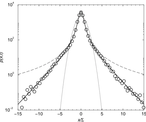
In Fig. 2 we plot the probability density p(x, t) of the S&P 500 cash index returns X(t) observed at time t = 1 min (circles). Σ = 1.87 × 10⁻⁴ is the
standard deviation of the empirical data. Dotted line corresponds to a Gaus-sian density with standard deviation given by Σ. Solid line shows the Fourier inversion of Eq. (12) with α = 1.30, σm = 9.07 × 10⁻⁴, and a = 2.97 × 10⁻³.
We use the gamma distribution of the absolute value of jump amplitudes, h(u) = µβ|u|β−1e−µ|u|/2Γ(β), (21)
with β = 2.39, and µ = qβ(β + 1) = 2.85. Dashed line represents a sym-metrical L´evy stable distribution of index α = 1.30 and the scale factor k = 4.31 × 10⁻⁶ obtained from Eq. (14). We note that the values of σ
m and Σ
predict that the Pareto-L´evy distribution fails to be an accurate description of the empirical pdf for x ≫ 5Σ (see Eq. (20)).
We chose a gamma distribution of jumps because (i) as suggested by the em-pirical data analized, the tails of p(x, t) decay exponentially, and (ii) one does not favor too small size jumps, i.e., those jumps with almost zero amplitudes.
−15 −10 −5 0 5 10 15 x/Σ 10−2 100 102 104 p(x,t)
Fig. 2. Probability density function p(x, t) for t = 1 min. Circles represent empirical data from S&P 500 cash index (January 1988 to December 1996). Σ is the standard deviation of empirical data. Dotted line corresponds to the Guassian density. Dashed line is the L´evy distribution and the solid line is the Fourier inversion of Eq. (22) with a gamma distribution of jumps (see main text for details).
In any case, it would be very useful to get some more microscopic approach (based, for instance, in a “many agents” model [3,22]) giving some inside on the particular form of h(u).
4 Conclusions
Summarizing, by means of a continous description of random pulses, we have obtained a dynamical model leading to a probability distribution for the spec-ulative price changes. This distribution which is given by the following char-acteristic function: ˜ p(ω, t) = exp −a 1 Z 0 z−1−α[1 − ˜h(ωzσm(t))]dz , (22)
where σm(t) = (bt)1/α, it depends on three positive constants: a, b, and α < 2.
the unit-variance characteristic function of jumps, also to be conjectured and fitted from the tails of the empirical distribution. Therefore, starting from simple and reasonable assumptions we have developed a new stochastic process that possesses many of the features, i. e. fat tails, self-similarity, superdiffusion, and finite moments, of financial time series, thus providing us with a different point of view on the dynamics of the market. We finally point out that the model does not explain any correlation observed in empirical data (as some markets seem to have [4,23]). This insufficiency is due to the fact that we have modelled the behavior of returns through a mixture of independent sources of white noise. The extension of the model to include non-white noise sources and, hence, correlations will be presented soon.
Acknowledgements
This work has been supported in part by Direcci´on General de Investigaci´on Cient´ıfica y T´ecnica under contract No. PB96-0188 and Project No. HB119-0104, and by Generalitat de Catalunya under contract No. 1998 SGR-00015.
References
[1] The Random Character of Stock Market Prices, P.H. Cootner ed. (MIT Press, Cambridge MA, 1964).
[2] M.G. Kendall, J. Royal Stat. Soc. 96, 11-25 (1953).
[3] J.Y. Campbell, A.W. Lo, and A.C. MacKinlay, The Econometrics of Financial Markets (Princeton University Press, Princeton, 1997).
[4] J.P. Bouchaud, and M. Potters, Th´eorie des Riskes Financiers (Al´ea-Saclay, Paris, 1997).
[5] B. Mandelbrot, J. Business 35, 394-419 (1963).
[6] W. Feller, An Introduction to Probability Theory and its Applications (J. Wiley, New York, 1971).
[7] R. N. Mantegna, and E.H. Stanley, Nature 376, 46-49 (1995). [8] E. Scalas, Physica A 253, 394-402 (1998).
[9] S. Gashghaie, W. Breymann, J. Peinke, P. Talkner, and Y. Dodge, Nature 381, 767-770 (1996).
[10] S. Gallucio, G. Caldarelli, M. Marsili, and Y.-C. Zhang, Physica A 245, 423-436 (1997).
[11] E. Fama, J. Business 35, 420-429 (1963).
[12] R.N. Mantegna, and E.H. Stanley, Phys. Rev. Lett. 73, 2946-2949 (1994). [13] I. Koponen, Phys. Rev. E 52, 1197-1199 (1995).
[14] T. Bollerslev, R.Y. Chou, and K.F. Kroner, J. Econometrics 52, 5-59 (1992). [15] R.F. Engle, Econometrica 50, 987-1007 (1982).
[16] T. Bollerslev, J. Econometrics 31, 307-327 (1986). [17] R.C. Merton, J. Financial Economics 3, 125-144 (1976). [18] J. Masoliver, Phys. Rev. A 35, 3918-3928 (1987).
[19] S.O. Rice, in Noise and Stochastic Processes, N. Wax ed. (Dover, New York, 1954).
[20] R.N. Mantegna, and E.H. Stanley, Nature 383, 587-588 (1996). [21] R. N. Mantegna, and E.H. Stanley, Physica A 239, 255-266 (1997). [22] T. Lux, and M. Marchesi, Nature 397, 498-500 (1999).
[23] A. W. Lo, and A. C. MacKinlay, Rev. Financial Studies 1, 41-66 (1988); 3, 175-205 (1990).