Int. J. of Thermodynamics ISSN 1301-9724 Vol. 11 (No. 2), pp. 49-60, June 2008
Nonlinear Generalization of Schrödinger's Equation
Uniting Quantum Mechanics and Thermodynamics
Gian Paolo Beretta
Università di Brescia, via Branze 38, 25123 Brescia, Italy
E-mail: [email protected]
Abstract
The nonlinear equation of motion that accomplishes a self-consistent unification of
quantum mechanics (QM) and thermodynamics conceptually different from the (von
Neumann) foundations of quantum statistical mechanics (QSM) and (Jaynes) quantum
information theory (QIT), but which reduces to the same mathematics for the
thermodynamic equilibrium (TE) states, and contains standard QM in that it reduces to the
time-dependent Schrödinger equation for zero entropy states is discussed in full
mathematical detail. By restricting the discussion to a strictly isolated system
(non-interacting, disentangled and uncorrelated), we show how the theory departs from the
conventional QSM/QIT rationalization of the second law of thermodynamics, which
instead emerges in QT (quantum thermodynamics) as a theorem of existence and
uniqueness of a stable equilibrium state for each set of mean values of the energy and the
number of constituent particles. To achieve this, the theory assumes
−kBTrρlnρfor the
physical entropy and is designed to implement two fundamental ansatzs: (1) that in
addition to the standard QM states described by idempotent density operators (zero
entropy), a strictly isolated and uncorrelated system admits also states that must be
described by non-idempotent density operators (nonzero entropy); (2) that for such
additional states the law of causal evolution is determined by the simultaneous action of a
Schrödinger-von Neumann-type Hamiltonian generator and a nonlinear dissipative
generator which conserves the mean values of the energy and the number of constituent
particles, and in forward time drives the density operator in the 'direction' of steepest
entropy ascent (maximal entropy generation). The resulting dynamics is well defined for all
non-equilibrium states, no matter how far from TE. Existence and uniqueness of solutions
of the Cauchy initial value problem for all density operators implies that the equation of
motion can be solved not only in forward time, to describe relaxation towards TE, but also
in backward time, to reconstruct the 'ancestral' or primordial lowest entropy state or limit
cycle from which the system originates. Zero entropy states as well as a well defined
family of non-dissipative states evolve unitarily according to pure Hamiltonian dynamics
and can be viewed as unstable limit cycles of the general nonlinear dynamics.
Keywords: second law of thermodynamics, irreversibility, nonunitary quantum dynamics,
maximal entropy generation, steepest entropy ascent, nonequilibrium relaxation, quantum
thermodynamics.
1. Thermodynamics after Prigogine
The non-orthodox unified quantum theory of mechanics and thermodynamics we discuss in this paper accomplishes from a different perspective the program that Prigogine and co-authors of the Brussels school set out during the same
decade,1976-1986, to seek a formulation of physical foundations whereby entropy and
irreversibility emerge from microscopic
kinematics and dynamics. For this reason, even though our approach is very different from that of the Prigogine school, I suggest that in a broad sense it does accomplish what Prigogine always felt it ought to be possible to do: to formulate a theory in which entropy emerges as an intrinsic objective physical property of matter and irreversibility as an objective dynamical aspect of microscopic physical reality.
We called our theory quantum thermodynamics (QT). It is noteworthy however
Int. J. of Thermodynamics, Vol. 11 (No. 2) 50
that the same term has been later used by many authors with different meanings. The two fundamental ansatzs of our QT were formulated in a series of papers published since 1976 by various members of the Keenan School of Thermodynamics at MIT (Keenan, Hatsopoulos, Gyftopoulos, Park, Beretta, Zanchini, Çubukçu, von Spakovsky). The theory has been defined “an adventurous scheme which seeks to incorporate thermodynamics into the quantum laws of motion, and may end arguments about the arrow of time – but only if it works” by J. Maddox, Nature, Vol.316, 11 (1985), and it has been recently rediscovered and re-evaluated by S. Gheorghiu-Svirschevski, Phys. Rev. A, Vol. 63, 054102 (2001).
Several authors have attempted to construct a microscopic theory that includes a formulation of the second law of thermodynamics [1, 2, 3, 4, 5, 6, 7, 8]. Some approaches strive to derive irreversibility from a change of representation of reversible unitary evolution, others from a change from the von Neumann entropy functional to other functionals, or from the loss of information in the transition from a deterministic system to a probabilistic process, or from the effect of coupling with one or more heat baths.
We discuss the key elements and features of a different non-standard theory which introduces de facto an ansatz of “intrinsic entropy and instrinsic irreversibility” at the fundamental level [9, 10], and an additional ansatz of ”steepest entropy ascent” which entails an explicit well behaved dynamical principle and the second law of thermodynamics. To present it, we first discuss an essential fundamental concept.
2. States of a strictly isolated individual system Let us consider a systemAand denote byR
the rest of the universe, so that the Hilbert space of the universe is HAR=HA⊗HR. We restrict our attention to a “strictly isolated” system Aby which we mean that at all times, −∞< t<∞, A
is uncorrelated (and hence disentangled) from R, i.e., ρAR=ρA⊗ρR, and non-interacting, i.e.,
R A R A AR H I I H H = ⊗ + ⊗ .
Many would object at this point that with this premise the following discussion should be dismissed as useless and unnecessary, because no “real” system is ever strictly isolated. We reject this argument as counterproductive, misleading and irrelevant, for we recall that physics is a conceptual edifice by which we attempt to model and unify our perceptions of the empirical world (physical reality [11]). Abstract concepts such as that of a strictly isolated system and that of a state of an individual system not only are well defined
and conceivable, but have been keystones of scientific thinking, indispensable for example to structure the principle of causality. In what other framework could we introduce, say, the time-dependent Schrödinger equation?
Because the dominant theme of quantum theory is the necessity to accept that the notion of state involves probabilistic concepts in an essential way [12], established practices of experimental science impose that the construct “probability” be linked to the relative frequency in an “ensemble”. Thus, the purpose of a quantum theory is to regularize purely probabilistic information about the measurement results from a “real ensemble” of identically prepared identical systems. An important scheme for the classification of ensembles, especially emphasized by von Neumann [13], hinges upon the concept of ensemble “homogeneity”. Given an ensemble it is always possible to conceive of it as subdivided into many sub-ensembles. An ensemble is homogeneous if every conceivable subdivision results in sub-ensembles all identical to the original (two sub-ensembles are identical if upon measurement of both of the same physically observable at the same time instant, the outcomes yield the same arithmetic mean, and this holds for all conceivable physical observables). It follows that each individual member system of a homogeneous ensemble has exactly the same intrinsic characteristics as any other member, which therefore define the “state” of the individual system. In other words, the empirical correspondent of the abstract concept of “state of an individual system” is the homogeneous ensemble (sometimes called “pure” [14, 15, 16] or “proper” [17, 18]).
We restrict our attention to the states of a strictly isolated individual system. By this we rule out from our present discussion all heterogeneous preparations, such as those considered in QSM and QIT, which are obtained by statistical composition of different homogeneous component preparations. Therefore, we concentrate on the intrinsic characteristics of each individual system and their irreducible, non-statistical probabilistic nature.
3. Broader quantum kinematics ansatz
According to standard QM the states of a strictly isolated individual system are in one-to-one correspondence with the one-to-one-dimensional orthogonal projection operators on the Hilbert space of the system. We denote such projectors by the symbolP. If |ψ〉 is an eigenvector ofP such that P|ψ =|〉 ψ〉 and 〈ψ |ψ〉=1 then P=|ψ 〉〈ψ |. It is well known that different from classical states, quantum states are characterized by irreducible intrinsic probabilities. We need not elaborate
further on this point. We only recall that 0 = ln TrP P − .
Instead, we adhere to the ansatz [19] that the set of states in which a strictly isolated individual system may be found is broader than conceived in QM, specifically that it is in one-to-one correspondence with the set of linear operators ρ on H , with ρ =† ρ, ρ>0, Trρ=1, without the restriction ρ =2 ρ. We call these the “state operators” to emphasize that they play the same role that in QM is played by the projectorsP , and that they are associated with the homogeneous preparation schemes. This fundamental ansatz was first proposed by Hatsopoulos and Gyftopoulos [19]. It allows an implementation of the second law of thermodynamics at the fundamental level in which the physical entropy, given by
ρ ρ ρ)= Tr ln
( kB
s − , emerges as an intrinsic microscopic and non-statistical property of matter, in the same sense as the (mean) energy
H
e(ρ)=Trρ is an intrinsic property.
We first assume that our isolated system is an indivisible constituent of matter, i.e., one of the following:
• A single strictly isolated d -level particle, in which case
k e d k d H H H= =⊕ =0 where k
e is the k -th eigenvalue of the (one-particle) Hamiltonian H and 1
k e
H the corresponding eigenspace). Even if the system is isolated, we do not rule out fluctuations in energy measurement results and hence we do not assume a “microcanonical” Hamiltonian (i.e.,
k e kP e H ~ ~
= H for somek~) but we assume a full
“canonical” Hamiltonian k e k ke P H H= 1=
∑
H .• A strictly isolated ideal Boltzmann gas of non-interacting identical indistinguishable d-level particles, in which case H is a Fock space,
n d n d
F ⊕∞ H⊗
H= = =0 . Again, we do not rule out
fluctuations in energy nor in the number of particles, and hence we do not assume a canonical number operator (i.e., z
d P z N=~ ⊗~
H for some z~)
but we assume a full grand canonical number
operator n
d n nP
N =
∑
∞=0 H⊗ and a full Hamiltonian n d n n H P H =∑
∞=0 H⊗ where J J n J n H I H =∑
=1( 1) ⊗is the n -particle Hamiltonian on Hd⊗n, (H )1 J
denotes the one-particle Hamiltonian on the J-th particle space (Hd)J and I the identity operator J
on the direct product space ⊗nK=1,K≠J(Hd)K of all
other particles. Note that [H,N]=0.
• A strictly isolated ideal Fermi-Dirac or Bose-Einstein gas of non-interacting identical indistinguishable
d
-level particles, in which caseH is the antisymmetric or symmetric subspace, respectively, of the Boltzmann Fock space just defined.
We further fix ideas by considering the simplest quantum system, a 2-level particle, a qubit. It is well known [20] that using the 3-vector
) , , (
= σ1 σ2 σ3
σ of Pauli spin operators,
l lσ ε σ σj, k]= jk
[ , we can represent the
Hamiltonian operator as = ( ) 2
1 σ
ω I+ h⋅
H h
where h is a unit-norm 3-vector of real scalars
) , ,
(h1 h2 h3 , and the density operators as
σ ρ I+ r⋅
2 1
= where r is a 3-vector of real scalars (r1,r2,r3) with norm r=|r|≤1, and
1 =
r ifρ is idempotent, ρ =2 ρ.
If the 2-level particle is strictly isolated, its states in standard QM are one-to-one with the unit-norm vectors ψ in H or, equivalently, the unit-trace one-dimensional projection operators on H,
| |
=|ψ ψ ψ 1ψ
ψ 〉〈 〉− 〈
P , i.e., the idempotent density operators ρ =2 ρ. Hence, in the 3-dimensional euclidean space (r1,r2,r3), states map one-to-one with points on the unit radius 2-dimensional spherical surface, r=1, the “Bloch sphere“. The mean value of the energy is
) (1 = Tr = ) ( 2 1 r h⋅ + H
eρ ρ and is clearly bounded by 0≤e(ρ)≤hω. The set of states that share a given mean value of the energy is represented by the one-dimensional circular intersection between the Bloch sphere and the constant mean energy plane orthogonal to h defined by the h⋅r= const condition. The time evolution according to the Schrödinger equation ψ&=−iHψ/h or, equivalently, P&ψ =−i[H,Pψ]/h or [20] r&=ωh×r yields a periodic precession of r around h along such one-dimensional circular path on the surface of the Bloch sphere. At the end of every (Poincaré) cycle the strictly isolated system passes again through its initial state: a clear pictorial
manifestation of the reversibility of Hamiltonian dynamics.
At the level of a strictly isolated qubit, the Hatsopoulos-Gyftopoulos ansatz amounts to accepting that the two-level system admits also states that must be described by points inside the
Int. J. of Thermodynamics, Vol. 11 (No. 2) 52
Bloch sphere, not just on its surface, even if the qubit is noninteracting and uncorrelated. The eigenvalues of ρ are (1±r)/2, therefore the isoentropic surfaces are concentric spheres,
+ + + − − − 2 1 ln 2 1 2 1 ln 2 1 = ) ( = ) ( sr k r r r r s ρ B (1)
The highest entropy state with given mean energy is at the center of the disk obtained by intersecting the Bloch sphere with the corresponding constant energy plane. Such states all lie on the diameter along the direction of the Hamiltonian vector h and are thermodynamic equilibrium (maximum entropy principle [21]).
Next, we construct our extension of the Schrödinger equation of motion valid inside the Bloch sphere. By assuming such a law of causal evolution, the second law will emerge as a theorem of the dynamics.
4. Steepest-entropy-ascent ansatz
Let us return to the general formalism for a strictly isolated system. We go back to the qubit example at the end of the section.
As a first step to force positivity and hermiticity of the state operator ρ we assume an equation of motion of the form
ρ ρ ρ ρ ρ ρ ρ ρ ρ ρ ρ = ( ) †( ) = ( ( )) ( ( ))† d d E E E E t + + (2) where E(ρ) is a (non-hermitian) operator-valued (nonlinear) function of ρ that we call the “evolution” operator. Without loss of generality, we write E=E++iE− where E+=(E+E†)/2
and E−=(E−E†)/2i are hermitian operators, so that Equation (2) takes the form
} ), ( { ] ), ( [ = d d ρ ρ ρ ρ ρ + − + −i E E t (3)
with [ ⋅⋅ and ,] { ⋅⋅,} the usual commutator and anti-commutator, respectively.
We consider the real space of linear (not necessarily hermitian) operators on H equipped with the real scalar product
)/2 ( Tr = ) | (F G F†G+G†F (4) so that for any time-independent hermitian observable X on H, the rate of change of the mean value x(ρ)=Tr(ρX)=( ρ | ρX) can be written as X E X
)
t t r ρ ρ ρ ρ | ( 2 = ) d d ( Tr = d ) ( d (5)from which it follows that a set of xi(ρ)'s is time invariant if ρEis orthogonal to the (real) linear span of the set of operators ρXi, that we denote by L{ ρXi}.
For an isolated system, we therefore require that, for every ρ, operator ρEbe orthogonal [in the sense of scalar product (4)] to the linear manifold L( ρI,{ ρRi}) where the set
} { , Ri I ρ
ρ always includes ρI , to preserve 1
=
Trρ , and ρH , to conserve the mean energy H
e(ρ)=Trρ . For a field of indistinguishable particles we also include ρN to conserve the mean number of particles n(ρ)=TrρN. For a free particle we would include ρPx, ρPy, ρPz
to conserve the mean momentum vector P
p(ρ)=Trρ , but here we omit this case for simplicity [30].
Similarly, the rate of change of the entropy functional can be written as
[
]
(
ρ ρ ρ ρ)
ρ ln 2 = d ) ( d − + B k E t s (6)where the operator−2kB
[
ρ + ρlnρ]
may be interpreted as the gradient (in the sense of the functional derivative) of the entropy functionalρ ρ ρ)= Tr ln
( kB
s − with respect to operator ρ (for the reasons why in our theory the physical entropy is represented by the von Neumann functional, see Refs. [19, 22]).
It is noteworthy that the Hamiltonian evolution operator
h / = iH
EH (7)
is such that ρEH is orthogonal to ))
(, ,
( ρI ρH ρN
L as well as to the entropy gradient operator −2kB
[
ρ + ρlnρ]
. It yields a Schrödinger-Liouville-von Neumann unitary dynamics ] , [ = = d dρ ρ †ρ ρ H i E E t H+ H −h (8)which maintains time-invariant all the eigenvalues of ρ. Because of this feature, all time-invariant
(equilibrium) density operators according to Equation (8) (those that commute with H ) are globally stable [23] with respect to perturbations that do not alter the mean energy (and the mean number of particles). As a result, for given values of the mean energy e(ρ) and the mean number of particles n(ρ) such a dynamics would in general imply many stable equilibrium states, contrary to the second law requirement that there must be only one (this is the well known Hatsopoulos-Keenan statement of the second law [24], which entails [21] the other well known statements by Clausius, Kelvin and Carathéodory).
Therefore, we assume that in addition to the Hamiltonian term E , the evolution operator E H has an additional component E , D
D
H E
E
E= + (9)
that we will take so that ρED is at any ρ orthogonal both to ρEH and to the intersection of the linear manifold L( ρI,{ ρRi}) with the isoentropic hypersurface to which ρ belongs (for a two-level system, such intersection is a one-dimensional planar circle inside the Bloch sphere). In other words, we assume that ρED is
proportional to the component of the entropy gradient operator −2kB
[
ρ + ρlnρ]
orthogonal to L( ρI,{ ρRi}),[
ln]
( , (, )) ) ( 2 1 = I H N D E ρ ρ ρ ρ ρ ρ τ ρ − ⊥L (10)where we denote the ”constant” of proportionality by 1/2τ(ρ) and use the fact that ρ has no component orthogonal to L( ρI, ρH(, ρN)). It is important to note that the “intrinsic dissipation” or “intrinsic relaxation” characteristic time τ(ρ) is left unspecified in our construction and need not be a constant. All our results hold as well if τ(ρ) is some reasonably well behaved positive definite functional of ρ. The empirical and/or theoretical determination of τ(ρ) is a most challenging open problem in our research program. For example, it has been suggested [25] that the experiments by Franzen [26] (intended to evaluate the spin relaxation time constant of vapor under vanishing pressure conditions) and by Kukolich [27] (intended to provide a laboratory
validation of the time-dependent Schrödinger equation) both suggest some evidence of an intrinsic relaxation time.
Using standard geometrical notions, we can show [9, 10, 28, 29] that given any set of linearly independent operators ρI,{ ρRi} spanning
)) (, ,
( ρI ρH ρN
L , the dissipative evolution operator takes the explicit expression
) ( ) ( 2 1 = ρ ρ ρ τ ρ M k E B D ∆ (11)
where M(ρ) is a “Massieu-function” operator defined by the following ratio of determinants
}) { , ( ) | ) | ) | ) | ) | ) | = ) ( ( ( ( ( ( ( i i i i i i i R I R R R I R S I R I I I S R I S M ρ ρ ρ ρ ρ ρ ρ ρ ρ ρ ρ ρ ρ ρ ρ Γ O M O M M L L O M O M M L L L L (12) in which we use the following notation (F , G hermitian) ρ ρln = kBPRan S − (13) I F r F F= −T (ρ ) ∆ (14) }) , { ( T 2 1 = ) | ( = G F r G F G F ∆ ∆ ∆ ∆ 〉 ∆ ∆ 〈 ρ ρ ρ (15) ] [ det = }) ({ = }) { , ( 〉 ∆ ∆ 〈 ∆ Γ Γ j i i i R R R R I ρ ρ ρ (16)
where Γ({ ρXi}) denotes the Gram determinant
)] |
[(
det ρXi ρXj .
The Massieu-function operator defined by Equation (12) generalizes to any non-equilibrium state the well known equilibrium Massieu characteristic function )] ( [ ) ( ) ( TE e TE n TE s ρ −β ρ +βµ ρ .
As a result, our full equation of motion
} ), ( { ) ( 2 1 ] , [ = d d ρ ρ ρ τ ρ ρ M k H i t B ∆ + − h (17)
Int. J. of Thermodynamics, Vol. 11 (No. 2) 54 . ] [ det } , { } , { } , { ) ( 2 1 ] , [ = d d 1 1 1 1 1 1 〉 ∆ ∆ 〈 〉 〉 〉 〉 〉 〉 + + − ∆ ∆ 〈 ∆ ∆ 〈 ∆ ∆ 〈 ∆ ∆ 〈 ∆ ∆ 〈 ∆ ∆ 〈 ∆ ∆ ∆ j i i R i R i R R i R S R i R R R R S i R R S B R R k H i t O M O M M L L O M O M M L L L L h ρ ρ ρ ρ τ ρ ρ (18) Eqs. (28a) and (28b) below show the explicit
forms when the set { ρRi} is empty or contains only operator ρH, respectively.
Gheorghiu-Svirschevski [30] re-derived our nonlinear equation of motion from a variational principle that in our notation may be cast as follows [29], ) ( = ) | ( and 0 = d ) ( d to subject d ) ( d max 2 ρ ρ ρ ρ ρ ρ c E E t r t s D D i D E (19) where r0(ρ)=Trρ, r1(ρ)=TrHρ , [r2(ρ)=TrNρ], and c2(ρ) is some positive functional. The last constraint means that we are not really searching for “maximal entropy production” but only for the direction of steepest entropy ascent, leaving unspecified the rate at which such direction “attracts” the state of the system. The necessary condition in terms of Lagrange multipliers is , 0 = ) | ( d d d d 0 D D D i D i i D E E E t r E t s E ρ ρ ρ λ ρ λ ρ ∂ ∂ − ∂ ∂ − ∂ ∂
∑
(20)and, using Eqs. (5) and (6) becomes
, 0 = 2 2 ) ln ( 2 0 D i i B E R k ρ λ ρ λ ρ ρ ρ − − + −
∑
(21)which inserted in the constraints and solved for the multipliers yields Equation (11).
The resulting rate of entropy change (entropy generation by irreversibility, for the system is isolated) is given by the equivalent expressions
(
D D)
B B E E k t r k t s ρ ρ ρ τ ρ ρ ρ ) ( 4 = d ln dT = d ) ( d − (22) }) { , ( }) { , , ln ( ) ( = i i R I R I kB ρ ρ ρ ρ ρ ρ ρ τ Γ Γ (23) . 0 }) { , ( }) { , , ( ) ( 1 = ≥ Γ Γ i i R I R I S kB ρ ρ ρ ρ ρ ρ τ (24)Because a Gram determinant ] [ det = ) , , ( 1 〈∆ ∆ 〉 Γ ρX K ρXN Xi Xj is either strictly positive or zero if operators { ρXi} are linearly dependent, the rate of entropy generation is either a positive semi-definite nonlinear functional of ρ, or it is zero if operators
) (, ,
, I H N
S ρ ρ ρ
ρ are linearly dependent, i.e., if the state operator is of the form
)]) ( [ exp ( Tr )] ( [ exp = N H B B N H B ν β ν β ρ + − + − (25)
for some “binary” projection operator B(B =2 B, eigenvalues either 0 or 1) and some real scalar(s)
β (and ν). Non-dissipative states are therefore all and only the density operators that have the nonzero eigenvalues “canonically” (or “grand canonically”) distributed. For them, ρED=0
and our equation of motion (17) reduces to the Schrödinger-von Neumann form i &hρ =[H,ρ].
Such states are either equilibrium states, if 0
= ] ,
[B H , or belong to a limit cycle and undergo a unitary Hamiltonian dynamics, if [B,H]≠0, in which case )]] ( [ exp ) ( [ Tr ) ( )] ( [ exp ) ( = ) ( N H t B t B N H t B t ν β ν β ρ + − + − (26) ) / ( exp = ) ( , ) ( (0) ) ( = ) (t U t B U 1 t U t itHh B − − (27)
For TrB=1 the states (25) reduce to the (zero entropy) states of standard QM, and obey the standard unitary dynamics generated by the usual time-dependent Schrödinger equation. For B =I
we have the maximal-entropy (thermodynamic-equilibrium) states, which turn out to be the only globally stable equilibrium states of our dynamics, so that the Hatsopoulos-Keenan statement of the second law emerges as an exact and general dynamical theorem.
Indeed, in the framework of our extended theory, all equilibrium states and limit cycles that
have at least one null eigenvalue of ρ are unstable. This is because any neighboring state operator with one of the null eigenvalues perturbed (i.e., slightly “populated”) to a small value ε (while some other eigenvalues are slightly
changed so as to ensure that the perturbation preserves the mean energy and the mean number of constituents), would eventually proceed “far away” towards a new partially-maximal-entropy state or limit cycle with a canonical distribution which fully involves also the newly “populated” eigenvalue while the other null eigenvalues remain zero.
It is clear that the canonical (grand-canonical) density operators
)]) ( [ exp ( T )]/ ( [ exp = H N r H N TE β ν β ν ρ − + − + are
the only stable equilibrium states, i.e., the TE states of the strictly isolated system. They are mathematically identical to the density operators which also in QSM and QIT are associated with TE, on the basis of their maximizing the von Neumann indicator of statistical uncertainty
ρ ρ ln Tr
− subject to given values of TrHρ (and
ρ
rN
T ). Because maximal entropy mathematics in QSM and QIT successfully represent TE physical reality, our theory, by entailing the same mathematics for the stable equilibrium states, preserves all the successful results of equilibrium QSM and QIT. However, within QT such mathematics takes up an entirely different physical meaning. Indeed, each density operator here does not represent statistics of measurement results from a “heterogeneous” ensemble, as in QSM and QIT where, according to von Neumann's recipe [13, 31], the “intrinsic” uncertainties (irreducibly introduced by standard QM) are mixed with the “extrinsic” uncertainties (related to the heterogeneity of its preparation, i.e., to not knowing the exact state of each individual system in the ensemble). In QT, instead, each density operator, including the maximal-entropy stable TE ones, represents “intrinsic” uncertainties only, because it is associated with a homogeneous preparation and, therefore, represents the state of each and every individual system of the homogeneous ensemble.
We noted elsewhere [33] that the fact that our nonlinear equation of motion preserves the null eigenvalues of ρ, i.e., conserves the cardinality
) ( Ker
dim ρ of the set of zero eigenvalues, is an important physical feature consistent with recent experimental tests (see the discussion of this point in Ref. [30] and references therein) that rule out, for pure (zero entropy) states, deviations from linear and unitary dynamics and confirm that initially unoccupied eigenstates cannot spontaneously become occupied. This fact, however, adds nontrivial experimental and conceptual difficulties to the problem of designing fundamental tests capable, for example, of ascertaining whether decoherence originates from uncontrolled interactions with the environment due to the practical impossibility of obtaining strict
isolation, or else it is a more fundamental intrinsic feature of microscopic dynamics requiring an extension of QM like the one we propose.
For a confined, strictly isolated d-level system, our equation of motion for non-zero entropy states (ρ ≠2 ρ) takes the following forms [20, 34]. If the Hamiltonian is fully degenerate [H =eI, e(ρ)=e for every ρ ],
(
ρ ρ ρ ρ ρ)
τ ρ ρ ln T ln 1 ] , [ = d d r H i t −h − − (28a)while if the Hamiltonian is nondegenerate,
2 2 2 ) T ( T T T ln T T 1 ln T } , { 2 1 ln 1 ] , [ = d d H r H r H r H r H r H r r H H i t ρ ρ ρ ρ ρ ρ ρ ρ ρ ρ ρ ρ ρ τ ρ ρ − − − − h (28b)
In particular, for a non-degenerate two-level system, it may be expressed in terms of the Bloch sphere representation (for 0<r<1) as [20]
2 2 ) ( 1 1 1 ln 2 1 1 = r h h r h r h r ⋅ − × × + − − − × r r r r τ ω & (29)
from which it is clear that the dissipative term lies in the constant mean energy plane and is directed towards the axis of the Bloch sphere identified by the Hamiltonian vector h. The nonlinearity of the equation does not allow a general explicit solution, but on the central constant-energy plane, i.e., for initial states with r⋅h=0, the equation implies [20] r r r r t + − − + − 1 1 ln 1 = 1 1 ln d d τ (30)
which, if τ is constant, has the solution
. (0) 1 (0) 1 ln exp tanh = ) ( + − − − r r t t r τ (31)
This, superposed with the precession around the Hamiltonian vector, results in a spiraling approach to the maximal entropy state (with entropy kBln2). Notice that the spiraling
trajectory is well defined and within the Bloch sphere for all times −∞< t<+∞, and if we follow it backwards in time it approaches as t→−∞ the limit cycle which represents the standard QM (zero entropy) states evolving according to the Schrödinger equation.
Int. J. of Thermodynamics, Vol. 11 (No. 2) 56
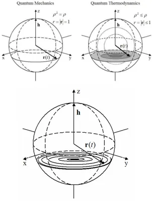
Figure 1. Pictorial representation of the augmented state space implied by the Hatsopoulos-Gyftopoulos ansatz with respect to
the state space of standard QM. For a strictly isolated and uncorrelated two-level system (qubit),
QM states are in one-to-one correspondence with the surface of the Bloch sphere, ρ2 = ρ, r = 1, so-called “pure states”; states in QT, instead, are in one-to-one correspondence with the entire sphere, surface and interior, ρ2 ≤ ρ, r ≤ 1; these are notthe “mixed states” of QSM/QIT. For a d-level strictly
isolated and uncorrelated system, the density operator ρ represents the state of the system, and the physical entropy S = – kBTr(ρlnρ) measures the
degree of sharing (internal distribution) of the energy among the available energy levels of the
system. The steepest-entropy-ascent (maximal-entropy-generation) dynamics given by the second
term in Equation (29) superposed with the precession around the hamiltonian vector due to
the first term in Equation (29), results in a spiraling approach to the maximal entropy state. The spiraling trajectory is well defined and within the Bloch sphere for all times −∞< t<+∞, and if we follow it backwards in time it approaches as
−∞ →
t the limit cycle which represents the standard QM (zero entropy) states evolving according to the Schrödinger equation of unitary
motion.
This example shows quite explicitly a general feature of our nonlinear equation of motion which follows from the existence and uniqueness of its solutions for any initial density operator both in forward and backward time. This feature is a
consequence of two facts: (1) that zero eigenvalues of ρ remain zero and therefore no eigenvalue can cross zero and become negative, and (2) that Tr ρ is preserved and therefore if initially one, it remains one. Thus, the eigenvalues of ρ remain positive and less than unity. On the conceptual side, it is also clear that our theory implements a strong causality principle by which all future as well as all past states are fully determined by the present state of the isolated system, and yet the dynamics is physically (thermodynamically) irreversible. Said differently, if we formally represent the general solution of the Cauchy problem by ρ(t)=Λtρ(0) the nonlinear map Λt is a group, i.e., Λt+u =ΛtΛu for all t and u , positive and negative. The map is therefore “invertible”, in the sense that Λ−t =Λ−t1, where the inverse map is defined by ρ(0)=Λ−t1ρ(t).
It is a nontrivial observation that the non-invertibility of the dynamical map is not at all necessary to represent a physically irreversible dynamics. Yet, innumerable attempts to build irreversible theories start from the assertion that in order to represent thermodynamic irreversibility the dynamical map should be non-invertible. The arrow of time in our view is not to be sought in the impossibility to retrace past history, but in the spontaneous tendency of any physical system to internally redistribute its energy (and, depending on the system, its other conserved properties such number of particles, momentum, angular momentum) along the path of steepest entropy ascent.
5. Onsager reciprocity
The intrinsically irreversible dynamics entailed by the dissipative (non-Hamiltonian) part of our nonlinear equation of motion also entails an Onsager reciprocity theorem. To see this, we first note that any density operator ρ can be written as [36] ) ( exp T ) ( exp = j j j j j j X f rB B X f B
∑
∑
− − ρ (32)where the possibly time-dependent Boolean B is such that B=PRanρ (=I−PKerρ) and the time-independent operators X together with the j identity I form a set such that their restrictions to
H
H'=B , {I′,X′j} span the real space of hermitian operators on H'=BH. Hence,
j j j X f f ρ ρ ρ ρln =− 0 −
∑
(33) ) ( T = ) ( j j r X x ρ ρ (34) ), ( = ) (ρ 0 j j ρ j x f k f k s B + B∑
(35) where ) ( ) ( ) ( = ρ ρ ρ j i x j j B x s f k ≠ ∂ ∂ (36)may be interpreted as a “generalized affinity” or force. Defining
)
. | ( 2 = D ) ( D i D i E X t x ρ ρ (37)as “the dissipative rate of change” of the mean value xj(ρ), we find , ) ( = D ) ( D ρ ρ ij j j i f L t x
∑
(38)where the coefficients Lij(ρ) (nonlinear in ρ) may be interpreted as “generalized conductivities” and are given explicitly (no matter how far ρ is from TE) by ) ] [ | ] [ ( = ) ( ) ( }) { , ( }) { , ( I Ri j I Ri i ij X X L ρ ρ ρ ρ ρ ρ ρ ρ τ L L ⊥ ⊥ (39) ) ( ) ( = ] [ det = 1 1 1 1 1 1 ρ ρ τ ji k k R k R k R R k R i X R k R R R R i X j X k R j X R j X i X L R R ∆ 〉 ∆ 〈 〉 〉 〉 〉 〉 〉 〉 〉 〉 ∆ ∆ 〈 ∆ ∆ 〈 ∆ ∆ 〈 ∆ ∆ 〈 ∆ ∆ 〈 ∆ ∆ 〈 ∆ ∆ 〈 ∆ ∆ 〈 ∆ ∆ 〈 l O M O M M L L O M O M M L L L L (40)
and therefore form a symmetric, non-negative definite Gram matrix [Lij(ρ)], which is strictly positive if all operators
}) { , ( ] [ i R I i X ρ ρ ρ ⊥L are linearly independent.
The rate of entropy generation may be rewritten as a quadratic form of the generalized affinities, . ) ( = d ) ( d ρ ρ ij j i j i L f f k t s B
∑
∑
(41) If all operators }) { , ( ] [ i R I i X ρ ρ ρ L ⊥ arelinearly independent, det[Lij(ρ)]≠0 and Equation (38) may be solved to yield
, D ) ( D ) ( = 1 t x L f ij i i j ρ ρ −
∑
(42)and the rate of entropy generation can be written also as a quadratic form of the dissipative rates
. D ) ( D D ) ( D ) ( = d ) ( d 1 t x t x L k t s i j ij j i B ρ ρ ρ ρ
∑
∑
− (43)6. Composite systems and reduced dynamics The composition of the system is embedded in the structure of the Hilbert space as a direct product of the subspaces associated with the individual elementary constituent subsystems, as well as in the form of the Hamiltonian operator. In this section, we consider a system composed of distinguishable and indivisible elementary constituent subsystems. For example:
• A strictly isolated composite of r distinguishable d -level particles, in which case
J d r J H H= ⊗ =1 and H H J IJ V r J ⊗ +
∑
( ) = =1 1where V is some interaction operator over H . • A strictly isolated ideal mixture of r types of Boltzmann, Fermi-Dirac or Bose-Einstein gases of non-interacting identical indistinguishable d -J level particles, J=1,K,r, in which case H is a composite of Fock spaces
r n r d n d r n n J d r J F ⊗ ⊗ ∞ ∞ ⊕ ⊗ ⊗ ⊕ ⊗ H H H L 1 L 1 0 = 0 = 1 1 = = =
where the factor Fock spaces belonging to Fermi-Dirac (Bose-Einstein) components are restricted to their antisymmetric (symmetric) subspaces. Again, we assume full grand-canonical number operators
J n J d J J n J n P N
∑
∞ ⊗ H 0 = = and Hamiltonian V P H I H J n J d J n J n J r J ⊗ ⊗ + ∞∑
∑
H 0 = 1 = = .For compactness of notation we denote the subsystem Hilbert spaces as
J J r H H H H H H= 1⊗ 2⊗L⊗ = ⊗ (44) where J denotes all subsystems except the J -th one. The overall system is strictly isolated in the sense already defined, and the Hamiltonian operator
Int. J. of Thermodynamics, Vol. 11 (No. 2) 58 V I H H J J r J + ⊗
∑
=1 = (45)where H is the Hamiltonian on J H associated J with the J -th subsystem when isolated and V (on
H) the interaction Hamiltonian among the r subsystems.
The subdivision into elementary constituents, considered as indivisible, and reflected by the structure of the Hilbert space H as a direct product of subspaces, is particularly important because it defines the level of description of the system and specifies its elementary structure. The system's internal structure we just defined determines the form of the nonlinear dynamical law proposed by this author [28, 29, 37] to implement the steepest entropy ascent ansatz in a way compatible with the obvious self-consistency “separability” and “locality” requirements [33]. It is important to note that because our dynamical principle is nonlinear in the density operator, we cannot expect the form of the equation of motion to be independent of the system's internal structure.
The equation of motion that we “designed” in [28, 37] so as to guarantee all the necessary features (that we list in Ref. [33]), is
J J J J J B r J M k H i t ρ ρ ρ ρ τ ρ ρ ⊗ ∆ + + −
∑
{( ( )) , } ) ( 2 1 ] , [ = d d 1 = h (46)where we use the notation [see Ref. [29] for interpretation of (S )J and (H )J]
[
( )]
( , ( ) (, ( ) )) = )) ( ( J kJ N J J J H J J I J J J J J J S M ρ ρ ρ ρ ρ ρ L ⊥ (47) )/2 ( T = ) | (FJ GJ J rJ FJ†GJ+G†JFJ (48) , ] ) [( T = ) (RiJ J rJ IJ⊗ρJ RiJ (49) , ] ) [( T = ) (S J rJ IJ⊗ρJ S (50) and the “internal redistribution characteristic times” τJ(ρ)'s are some positive constants or positive functionals of the overall system's density operator ρ .All the results found for the single constituent extend in a natural way to the composite system. For example, the rate of entropy change becomes
}) ) ( { , ( }) ) ( { , , ) ( ( ) ( 1 = d ) ( d =1 J J J iJ J J iJ J J J J J J B r J I R R I S k t s ρ ρ ρ ρ ρ ρ τ ρ Γ Γ
∑
(51) The dynamics reduces to the Schrödinger-von Neumann unitary Hamiltonian dynamics when, for each J, there are multipliers λiJ such that . ) ( = ) ( iJ iJ J i J J J S ρ λ R ρ∑
(52)The equivalent variational formulation is
, ) ( = ) | ( a 0 = d ) ( d d ) ( d max 2 } { ρ ρ ρ ρ ρ ρ J J DJ J DJ J i DJ E J c E E nd t r to subject t s (53) where r0(ρ)=Trρ , r1(ρ)=TrHρ [, ρ ρ rN
r2( )=T ], and c2J(ρ) are some positive functionals of ρ. The last constraints, one for each subsystem, mean that each subsystem contributes to the overall evolution (for the dissipative non-Hamiltonian part) by pointing towards its “local perception” of the direction of steepest (overall) entropy ascent, each with an unspecified intensity (which depends on the values of the functionals cJ(ρ), that are inversely related to the internal redistribution characteristic times
) (ρ τJ ).
If two subsystems A and B are non-interacting but in correlated states, the reduced state operators obey the equations
J A J J J J r J A J A A A M k H i t B ) ( } , )) ( {( ) ( 2 1 1 ] , [ = d d 1 = ρ ρ ρ ρ τ ρ ρ ⊗ ∆ + −
∑
∈ h (54) J B J J J J r J B J B B B M k H i t B ) ( } , )) ( {( ) ( 2 1 1 ] , [ = d d 1 = ρ ρ ρ ρ τ ρ ρ ⊗ ∆ + −∑
∈ h (55) where (ρA)J =TrJ(ρA), (ρB)J =TrJ(ρB), andoperators (∆MJ(ρ))J result independent of H B for every J ∈A and independent of H for every A
B
J ∈ . Therefore, all functionals of ρA (local observables) remain unaffected by whatever change in B , i.e., locality problems are excluded.
7. Concluding remarks
According to QSM and QIT, the uncertainties that are measured by the physical entropy are to be regarded as either extrinsic features of the heterogeneity of an ensemble or as witnesses of correlations with other systems. Instead, we discuss an alternative theory, QT, based on the Hatsopoulos-Gyftopoulos fundamental ansatz [19, 31] that also such uncertainties are irreducible (and hence, “physically real” and “objective” like standard QM uncertainties) in that they belong to the state of the individual system, even if uncorrelated and even if a member of a homogeneous ensemble.
According to QT, second law limitations emerge as manifestations of such additional physical and irreducible uncertainties. The Hatsopoulos-Gyftopoulos ansatz not only makes a unified theory of QM and thermodynamics possible, but gives also a framework for a resolution of the century-old “irreversibility paradox”, as well as of the conceptual paradox [31] about the QSM/QIT interpretation of density operators, which has preoccupied scientists and philosophers since Schrödinger surfaced it in Ref. [32]. This fundamental ansatz seems to respond to Schrödinger prescient conclusion in Ref. [32]: “in a domain which the present theory (quantum mechanics) does not cover, there is room for new assumptions without necessarily contradicting the theory in that region where it is backed by experiment.”
QT has been described as “an adventurous scheme” [38], and indeed it requires quite a few conceptual and interpretational jumps, but (1) it does not contradict any of the mathematics of either standard QM or TE QSM/QIT, which are both contained as extreme cases of the unified theory, and (2) for nonequilibrium states, no matter how “far” from TE, it offers the structured, nonlinear equation of motion proposed by this author which models, deterministically, irreversibility, relaxation and decoherence, and is based on the additional ansatz of steepest-entropy-ascent microscopic dynamics.
Many authors, in a variety of contexts [35], have observed in recent years that irreversible natural phenomena at all levels of description seem to obey a principle of general and unifying validity. It has been named [35] “maximum entropy production principle”, but we note in this paper that, at least at the quantum level, the weaker concept of “attraction towards the direction of steepest entropy ascent” [9, 10, 28] is sufficient to capture precisely the essence of the second law.
We finally emphasize that the steepest-entropy-ascent, nonlinear law of motion we
propose, and the dynamical group it generates (not just a semi-group), is a potentially powerful modeling tool that should find immediate application also outside of QT, namely, regardless of the dispute about the validity of the Hatsopoulos-Gyftopoulos ansatz on which QT hinges. Indeed, in view of its well defined and well behaved general mathematical features and solutions, our equation of motion may be used in phenomenological kinetic and dynamical theories where there is a need to guarantee full compatibility with the principle of entropy non-decrease and the second-law requirement of existence and uniqueness of stable equilibrium states (for each set of values of the mean energy, of boundary-condition parameters,and of the mean amount of constituents).
References
[1] V. Gorini and E.C.G. Sudarshan, in Foundations of Quantum Mechanics and Ordered Linear Spaces (Advanced Study Institute, Marburg, 1973), Editors A. Hartkämper and H. Neumann, Lecture Notes in Physics, Vol. 29, pp. 260-268.
[2] V. Gorini, A. Kossakowski and E.C.G. Sudarshan, J. Math. Phys. 17, 821 (1976). [3] G. Lindblad, Commun. Math. Phys. 48, 119
(1976).
[4] E.B. Davies, Rep. Math. Phys. 11, 169 (1977).
[5] H. Spohn and J. Lebowitz, Adv. Chem. Phys. 38, 109 (1978).
[6] R. Alicki, J. Phys. A 12, L103 (1979). [7] B. Misra, I. Prigogine, and M. Courbage ,
Proc. Natl. Acad. Sci. USA, 76, 3607, 4768 (1979).
[8] M. Courbage and I. Prigogine, Proc. Natl. Acad. Sci. USA, 80, 2412 (1983).
[9] G.P. Beretta, in Frontiers of Nonequilibrium Statistical Physics, proceedings of the NATO Advanced Study Institute, Santa Fe, June 1984, Editors G.T. Moore and M.O. Scully (NATO ASI Series B: Physics 135, Plenum Press, New York, 1986), p. 193 and p. 205. [10] G.P. Beretta, in The Physics of Phase Space,
edited by Y.S. Kim and W.W. Zachary (Lecture Notes in Physics 278, Springer-Verlag, New York, 1986), p. 441.
[11] H. Margenau, The Nature of Physical Reality, McGraw-Hill, 1950.
[12] J.L. Park, Am. J. Phys. 36, 211 (1968). [13] J. von Neumann, Mathematical Foundations
of Quantum Mechanics, Engl. transl. of the 1931 German edition by R.T. Beyer,
Int. J. of Thermodynamics, Vol. 11 (No. 2) 60
Princeton University Press, 1955, pp. 295-346.
[14] D. Bohm and J. Bub, Rev. Mod. Phys. 38, 453 (1966).
[15] J.L. Park, Philosophy of Science 35, 205, 389 (1968).
[16] W. Band and J.L. Park, Found. Phys. 1, 133 (1970).
[17] B. d'Espagnat, Conceptual Foundations of Quantum Mechanics, Addison-Wesley, second edition, 1976.
[18] C.G. Timpson and H.R. Brown, Int. J. Quantum Inf. 3, 679 (2005).
[19] G.N. Hatsopoulos and E.P. Gyftopoulos, Found. Phys. 6, 15, 127, 439, 561 (1976). [20] G.P. Beretta, Int. J. Theor. Phys. 24, 119
(1985).
[21] E.P. Gyftopoulos and G.P. Beretta, Thermodynamics: Foundations and Applications, Dover Publications, Mineola, NY, 2005.
[22] E.P. Gyftopoulos and E. Çubukçu, Phys. Rev. E 55, 3851 (1997).
[23] G.P. Beretta, J. Math. Phys. 27, 305 (1986). [24] The stable-equilibrium formulation of the
second law of thermodynamics is well known and must be traced to G. N. Hatsopoulos and J. H. Keenan, Principles of General Thermodynamics, Wiley, New York, 1965. It has been further clarified in J. H. Keenan, G. N. Hatsopoulos, and E. P. Gyftopoulos, Principles of Thermodynamics, in Encyclopaedia Britannica, Chicago, 1972, and fully developed in Ref. [21].
[25] E. Çubukçu, Sc.D. thesis, M.I.T., 1993, unpublished.
[26] W. Franzen, Phys. Rev. 115, 850 (1959). [27] S.G. Kukolich, Am. J. Phys. 36, 420 (1967). [28] G.P. Beretta, Sc.D. thesis, M.I.T., 1981,
unpublished, ArXiv:quant-ph/0509116. [29] G.P. Beretta, ArXiv:quant-ph/0112046. [30] S. Gheorghiu-Svirschevski, Phys. Rev. A 63,
022105, 054102 (2001).
[31] G.P. Beretta, Mod. Phys. Lett. A 21, 2799 (2006).
[32] E. Schroedinger, Proc. Cambridge Phil. Soc. 32, 446 (1936).
[33] G.P. Beretta, Mod. Phys. Lett. A 20, 977 (2005).
[34] G.P. Beretta, Phys. Rev. E 73, 026113 (2006).
[35] See, e.g., R.C. Dewar, J. Phys. A 38, L371 (2005); P. Županović, D. Juretić, and S. Botrić, Phys. Rev. E 70 056108 (2004); H. Ozawa, A. Ohmura, R.D. Lorentz, amd T. Pujol, Rev. Geophys. 41, 1018 (2003); H. Struchtrup and W. Weiss, Phys. Rev. Lett. 80, 5048 (1998); and Ref. [30].
[36] G.P. Beretta, Found. Phys. 17, 365 (1987). [37] G.P. Beretta, E.P. Gyftopoulos, J.L. Park, and
G.N. Hatsopoulos, Nuovo Cimento B 82, 169 (1984); G.P. Beretta, E.P. Gyftopoulos, and J.L. Park, Nuovo Cimento B 87, 77 (1985). [38] J. Maddox, Nature 316, 11 (1985).
[39] References [9, 10, 12, 20, 23, 25, 28, 36, 37, 38] are available online at