A Novel Look at Long-run Convergence Dynamics in the United States

(1)

A novel look at long-run convergence dynamics in the US

Margherita Gerolimetto and Stefano Magrini

Abstract

When regional disparities follow a cyclical short-run pattern, convergence analysis results can be sizeably distorted. To tackle this issue, we propose a method based on the extraction of the trend from regional income time series that eschews misleading results when the nature of the cyclical pattern changes over time. Using real per capita personal income data for 48 conterminous US states and the distribution dynamics approach, we identify three distinct consecutive phases: strong convergence (1930-1970), substantial persistence (1971-1980) and divergence (1981-2010).

Keywords

Convergence, Business-cycle, Regional disparities, Distribution dynamics, Time series trend extraction

Acknowledgements

We thank two anonymous referees whose insightful comments have greatly contributed to the quality of the analysis. Needless to say, all errors and remaining infelicities of style are our own responsibility.

This is the accepted version of the article published in the International

Regional Science Review on September 11, 2014

(2)

1

1 Introduction

Virtually all methods for the analysis of convergence share the same weakness: the object of interest to convergence analysts is, essentially, the evolution of (relative) potential output; since measured output is a noisy indicator of potential output, contaminated by business cycle dynamics, results can be biased.

The mechanism through which this weakness manifests its consequences differs according to the specific method chosen by the researcher. Within a time series perspective, business cycle fluctuations contaminate the way the growth process is modeled since the definition of stochastic convergence abstracts from cyclical components (Durlauf et al., 2005). Within a cross-sectional perspective, due to business cycle fluctuations characterizing the economies under study, income disparities might also tend to exhibit a cyclical pattern in the short-run. This, in turn, might introduce a bias in the results whenever the analyzed period includes an unequal number of expansions and downturns.

In the latter framework, the practical solution suggested in Magrini et al. (2013) is to confine the analysis to a time period that includes exactly one (or more) entire business cycles of the aggregate economy. To achieve its aim, this method requires that the nature of the cyclical pattern of the disparities does not change substantially over time and regional cycles are sufficiently synchronized. This way of tackling the issue is, however, somewhat rigid. Whenever a researcher cannot be sure that the cyclical pattern of the disparities has not modified its nature over the considered time span, the degree of cycle synchronization is low or, simply, when there is a specific interest in analyzing a time period that does not coincide with complete business cycles, the approach proposed in Magrini et al. (2013) cannot fruitfully be employed. In fact, Duran (2014) finds that income disparities across US states switch from counter- to pro-cyclical between the end of the 1980’s and the beginning of the

(3)

2

1990s and ascribes this to a combination of a process of structural transformation towards a knowledge based “new economy” and a change in the direction of factor flows. In addition, he shows that differences in timing of the states’ cycles gain in importance after the end of the 1980’s while the role of amplitude differences correspondingly declines. With these concerns in mind, in this paper we propose a different method that allows for short-run fluctuations of whatever nature (and even if it varies over time) and, at the same time, frees the researcher from the need to confine the analysis to periods stretching between corresponding turning-points of the cycle of the aggregate economy.

Here, we employ this new method to study the evolution of regional disparities in the US where a general pattern is not instantly recognizable as conflicting results are reported for the same spatial units and broadly similar time periods even when the same methodological approach is adopted. Within the regression approach, usually associated to the notion of β-convergence (Barro and Sala-i-Martin, 1991, 1992 and 1995),1

1_{The theoretical foundations of this notion of convergence lie in the traditional neoclassical growth model}

originally set out by Solow (1956) and Swan (1956). Within this approach, the parameter β represents the rate at which the representative economy approaches its steady-state growth path.

cross-section data analyses overwhelmingly report evidence of unconditional convergence (recent examples are: Rey and Montouri, 1999; Garofalo and Yamarik, 2002; Miller and Genc, 2005; Higgins et al., 2006; Papyrakis and Gerlagh, 2007; Checherita, 2009); in contrast, recent results based on panel data (Lall and Yilmaz, 2001; Shioji, 2001, Checherita, 2009; Yu and Lee, 2012) and time series (Kane, 2001; Tomljanovic and Vogelsang, 2001; Mello; 2011; Holmes et al., 2013) methods often describe a tendency for a variety of spatial units to converge towards multiple steady-states, i.e., conditional convergence. Ambiguous results are also found when the US context is analyzed using the distribution dynamics approach (Quah, 1993 a and b, 1996 a and b, 1997) where evidence of strong convergence (Quah, 1996a and 1997; Hammond and Thompson, 2002; Johnson, 2000; Yamamoto, 2008) coexists with polarization (Wang, 2004;

(4)

3 DiCecio and Gascon, 2010; Yu, 2012).

Among the possible reasons for these ambiguities, a few authors (Magrini, 1999; Pekkala, 2000; Petrakos et al., 2005) have suggested a role for short-run convergence dynamics related to the business cycle: whenever regional income disparities follow a distinct cyclical pattern in the short-run and the period of analysis features an unequal number of expansions and downturns, the over-represented dynamics might introduce a bias in the results. Indeed, this is clearly demonstrated by Magrini et al. (2013), who also find strong evidence of polarization in per capita personal income across US states when the analysis is restricted to a period that stretches exactly between two peaks of the US cycle (1989:Q1-2007:Q2) and in which the cyclical pattern of the disparities has not modified its nature.

From a policy perspective, we stress the importance to provide a clear distinction between a short-run component of the disparities, connected to business cycle fluctuations and possibly bound to vanish, and a long-run one, arguably with a more structural character. Indeed, findings of an increased role exerted by the long-run component of the disparities call for structural interventions aimed at nurturing an environment conducive to innovation and firm creation, at promoting the development of human capital and at encouraging infrastructure upgrading in strategic sectors. In contrast, in case of an increase in the short-run component of the disparities, the policy maker might consider the opportunity to resort to measures aimed at temporarily sustaining income in regions lagging behind.

The paper is structured as follows. Section 2 presents a new method for the analysis of convergence that allows for short-run fluctuations in the disparities. The validity of this method is then demonstrated in Section 3 through a comparison with the results for the

(5)

1989-4

2007 period documented in Magrini et al. (2013). In the same section, we also study convergence dynamics in the US using annual data on real personal per capita income for 48 conterminous states and identify three distinct phases: a phase of very strong convergence that runs from 1930 to 1970, a phase of substantial persistence across the oil crises and a phase of divergence between 1981 and 2010. Section 4 concludes.

2 Adopted Methodology

As argued at the outset, the object of interest to convergence analysts is, essentially, the evolution of (relative) potential output. Consider a set of N economies and, for each, a time series of length T representing the evolution over time of observed per capita income. To allow for short-run fluctuations in the analysis of convergence across the N economies, we propose a procedure in two steps. As a first step, in order to get an output measure that is not contaminated by the business cycle dynamics, we apply a band-pass filter to each of the N time series of observed per capita output. Then, once the N trends have been estimated, we fix two points, t and t+s, and study convergence dynamics over this specific time period applying the distribution dynamics approach to data on the extracted trends. The following sub-sections provide a brief description of the adopted method and discuss the way it is implemented in the present study.

2.1 Cycle and trend extraction

Probably the most common approach for studying the business cycle by separating trend and cyclical components from a time series is represented by band-pass filters. The logic underpinning this class of filters is to identify the cycle by removing components whose frequency is either too high (seasonality and noise) or too low (trend). Popular examples are the filters developed by Hodrick and Prescott (1997, HP filter hereafter), by Baxter and King

(6)

5

(1999, BK filter hereafter) and by Christiano and Fitzgerald (1999 and 2003, CF filter hereafter). Here, we opt for the HP filter because of its simplicity and, despite criticisms (see, among others, Canova, 1998; Gomez, 2001), its widespread use; at the same time, in order to evaluate the sensitivity of the results, we will also report results obtained from the use of BK and CF filters.

Assuming that a given time series yt involves a trend, ygt, and a cycle, yct, as in c t g t t y y y = + for t = 1, ..., T (1)

the estimation of the trend component via the HP filter requires the solution of the following minimization problem:

(

) (

)

[

]

∑

= − + − − + − T t g t g t g t g t t ytg 1 y y y y y 2 2 1 2 2 λ min (2)

for a given value of λ, the parameter that controls the degree of smoothness of the estimated trend and, consequently, the shape of the cyclical swings. Indeed, as λ increases, the estimated trend component approaches a linear function.

In general, λ = 1600 is considered as a default value in case of quarterly data. This comes from the seminal paper of Hodrick and Prescott (1997) who indicate it as a suitable choice for quarterly data on GDP for the US economy between 1959 and 1979. There is however a rich debate on its appropriateness (among others, Paige and Trinidade, 2010; Harvey and Trimbur, 2008; Marcet and Ravn, 2004; Ravn and Uhlig, 2002; Pedersen, 2001). In extreme synthesis, the interpretation of this parameter, and hence the criteria upon which its value is determined, varies according to the way the filter is conceived. In the original setup by Hodrick and Prescott, λ can be seen as the ratio between the variance of yc (the cyclical component) and the variance of the second difference of yg (the trend component). The authors do not estimate these variances; rather, on the prior that a 5 percent cyclical component is moderately large in

(7)

6

relation to one-eight of 1 percent change in the growth rate in a quarter, they obtain a value for λ equal to 1600:

( )

18 1600 5

λ= 2 ₂ =

Alternatively, the HP filter can be expressed as Butterworth type filter (Gomez, 2001). Within this framework, the filter assigns to the cycle all swings with frequency higher than ωc-o, the

so-called cut-out frequency; this cut-out frequency, in turn, is equal to 1/pc-o where pc-o

indicates the period of a complete business cycle. For any given value of ωc-o, it is then

possible to derive the corresponding λ as:

4 o c 2 ω sin 2 λ − −             = where 0 < ωc-o < π (3)

Following this interpretation, Gomez (2001) shows that the value of 1600 indicated by Hodrick and Prescott implies a cut-out period of 9.93 years or 39.7 quarters. In fact, the average cycle duration according to National Bureau of Economic Research (NBER) official dating is approximately 20 quarters during the time period considered by Hodrick and Prescott, i.e., about one-half of the cut-out implied by λ = 1600.

Kaiser and Maravall (1999) stress that the choice of λ must not only consider the period under analysis but also the interest of the researcher. Subscribing to this view, in the present context this implies that the value of λ must guarantee that all cyclical swings are effectively removed from the estimated trend component. When choosing the smoothing parameter we therefore take into account the following context-specific aspects: i. the actual average duration of the US business cycle over the period under analysis; ii. the fact that the US cycle is actually a weighted average of the states’ cycles and, as a consequence, the average cycle duration of some states might well exceed that of the nation; iii. the need that, for each state, also the cycles with the maximum duration are effectively removed. Naturally, the value of λ

(8)

7

determined in accordance with these aspects could be (substantially) larger than the traditional value of 1600.2 It should be stressed, however, that the squared second difference of the trend component in equation (2) is a very small term; hence, even very large changes in λ influence the cyclical component yc only modestly (Zarnowitz and Ozyldirim, 2006).

Finally, it must be noted that an important drawback of the HP filter, as well as of any signal extraction procedure (e.g., Baxter and King, 1999; Kaiser and Maravall, 1999), refers to the inaccuracy of its estimates at the endpoints of the available sample. In particular, end-of-sample estimates tend to be close to the observed data thus introducing cycle fluctuations into the estimated trend. To address this problem, usual solutions are: i. to expand the information set supplied to the filter by the use of forecasts (e.g., Garratt et al., 2008; Mise et al., 2005; Kaiser and Maravall, 1999, 2001); ii. to ignore estimates at sample endpoints. In the empirical analysis, we shall follow the latter strategy.

2.2 The Distribution Dynamics Approach

As mentioned in the introductory section, there are two broad approaches to the analysis of convergence: the regression and the distribution dynamics approach (for an account of this literature and relative merits see, among others Durlauf and Quah, 1999; Temple, 1999; Islam, 2003; Magrini, 2004 and 2009; Abreu et al. 2005; Durlauf et al., 2005). In our view, the most important drawback of the regression approach relates to its informative content: concentrating on the behavior of a representative economy, the best this approach can do is to describe how this economy converges to its own steady-state; in contrast, it does not provide information about what happens to the entire cross-sectional distribution of economies, both in terms of external shape and intra-distributional dynamics. For this reason, in the analysis

2_{This is not uncommon in the literature. For instance, starting from a different perspective, Harvey and}

Trimbur (2008) state that for the quarterly time series of the US investment, λ = 32000 is a much more appropriate value.

(9)

8

that follows we opt for the distribution dynamics approach (Quah, 1993 a and b, 1996 a and b, 1997), in which the evolution of the cross-sectional distribution of per capita income is examined directly, using stochastic kernels to describe both the change in the distribution’s external shape and the intra-distribution dynamics.

Let the random variables X and Y represent per capita income (relative to group average) of a group of N economies at time t and t+s respectively. Now, let F(X) and F(Y) represent the corresponding distributions and assume that each of them admits a density denoted respectively with f(X) and f(Y). Assuming that the dynamics of f(•) can be modeled as a first order process, the density at time t+s is given by:

( ) ( | ) ( )

f Y f Y X f X d X

∞ −∞

=

∫

(4)

in which f(Y|X) is the stochastic kernel, effectively a conditional density function, mapping the density at time t into the density at time t+s. The stochastic kernel is the element that allows performing the analysis of convergence within this approach: it provides information both on the evolution of the external shape of the income distribution and on intra-distributional dynamics, i.e. on the movement of the economies from one part of the distribution to another between time t and time t+s. Convergence can hence be analyzed directly from the shape of a plot of the stochastic kernel estimate or, assuming that the process behind (4) follows a time homogenous markov process, by comparing the shape of the initial distribution to the stationary (or ergodic) distribution which is the limit of f(Y) as s→∞.

Before proceeding with the discussion concerning the way in which the stochastic kernel can be estimated, a few comments on the hypothesis of time homogeneity appear worthwhile. A first relevant aspect is related to the assumption of time homogeneity within the period under analysis. From this viewpoint, Hierro and Maza (2009) note that in some instances

(10)

intra-9

distribution mobility may change over the considered time span and thus imposing stationarity might affect the result. To address the issue the authors then opt for the discretization of the income space thus simplifying the stochastic kernel in (4) into a transition probability matrix and then estimate the latter by applying the Chapman-Kolmogorov equation to include information on intermediate times. However, as commonly recognised in the literature, discretizing a continuous first-order Markov process is likely to remove the Markov property and, because of this, we prefer to eschew discretization and maintain a continuous income space. This choice, on the other hand, prevents us from adopting the approach suggested by Hierro and Maza (2009). That said, we also think that the concerns expressed by Hierro and Maza might be of lesser importance in the present study as, in our view, a likely source of distribution dynamics instability is represented by short-term, business cycle related dynamics, which we will actually filter away from the data.

A second relevant aspect regards the extension of the time homogeneity assumption after the period of analysis. From this viewpoint, although clearly unrealistic, time homogeneity is a somewhat “mechanical” assumption, unavoidable in order to calculate the ergodic distribution whose purpose, it must be emphasised, is to magnify the dynamics at play during the period under analysis, not to derive a forecast of what will happen in the future (Quah, 1993, footnote 4).

Moving now to the estimation issues, a common way to obtain an estimate of the stochastic kernel in equation (4) is through the kernel density estimator. However, Hyndman et al. (1996) argue that this estimator might have poor bias properties and, to overcome the problem, suggest to adjust the estimate of the mean function implicit in the kernel density estimator with one obtained from a smoother with better bias properties. In the present

(11)

10

analysis, therefore, we apply this mean-bias adjustment and, in particular, employ the local linear estimator (Loader, 1999) to obtain a superior estimate of the mean function.

Operatively, the estimation of a stochastic kernel with the mean bias adjustment requires the choice of three important parameters: the first two are the bandwidths needed in the estimate of the conditional density, the third is the bandwidth needed to estimate the mean function. To obtain all stochastic kernels we resort to a Gaussian kernel with a nearest-neighbor bandwidth in the initial year dimension (with a span of 30% of the data) and a fixed Normal Scale (Silverman, 1986) bandwidth in the final year dimension. Estimates of the mean functions are obtained via a local linear estimator with a nearest-neighbor bandwidth (with span chosen to minimize AIC). The output in the core empirical analysis is a set of figures: a three-dimensional plot of the estimated stochastic kernel, the corresponding contour plot (with contours at the 90%, 50% and 10% of the overall volume), the Highest Density Region (HDR) plot (proposed by Hyndman, 1996, and in which the vertical strips represent conditional densities for a specific value in the initial year dimension and, for each strip, darker to lighter areas display the 10%, 50% and 90% highest density regions), and a plot comparing the ergodic distribution with those in the initial and final years.

3 Empirical Results

We employ two datasets on real per capita personal income net of current transfer receipts for 48 conterminous states: the first contains quarterly data from the 1st quarter of 1969 to the 3rd quarter of 2012, the second contains annual data from 1929 to 2011.3

As explained in the previous section, we begin the analysis by extracting the trend from each

3_{Data on personal per capita income come from the Bureau of Economic Analysis, while the consumer price}

index comes from the Bureau of Labor Statistics. Data and Matlab codes employed in the analysis are freely available from Stefano Magrini’s personal website: https://sites.google.com/a/unive.it/smagrini/home.

(12)

11

of the 48 series using the HP filter and this, in turn, requires the choice of λ following the logic spelt out in section 2.1. To start off, we recall that the cut-out period implied by the choice of λ made by Hodrick and Prescott was approximately 40 quarters, i.e., about twice the duration of the average cycle according to the NBER official dating during the period under stud y. In our datasets, based on NBER dating, the average cycle duration over the period covered by annual data (1929-2011) is 25 quarters, when the cycle goes from one peak to the next, or 26 quarters, when the cycle goes from trough to trough. Instead, for the period covered by quarterly data (1969:Q1-2012:Q3), the average cycle duration is 24 quarters in both cases. Therefore, if we maintain the same proportion implicit in Hodrick and Prescott’s choice between average and cut-out cycles, the parameter should be fixed at a value corresponding to about 50 quarters yielding, through the formula in equation (3), a value of λ of 4021. As previously pointed out, however, the US cycle is in fact a weighted average of the states’ cycles and, for a given average duration at the national level, the average duration at the state level can be somewhat longer. Thus, since the value of λ must be able to remove all cycles from all state series, we suggest increasing the proportion between the average and the cut-out cycles to 2.5, leading to a value of λ of 9807. The analysis that follows is hence carried out imposing of 10000 for the HP parameter for quarterly data; for annual data, we follow the rule suggested by Ravn and Uhlig (2002), according to which the HP parameter is calculated from the value for quarterly data by multiplying it by 4-4, and obtain a value of 40.

3.1 Quarterly data

In this section, we employ the dataset consisting of the quarterly time series of real per capita personal income across US states to ascertain the ability of the proposed method to obtain results unaffected by the bias brought on by short-run dynamics related to the business cycle. To achieve this aim, we consider different sub-periods and, for each of them, estimate

(13)

12

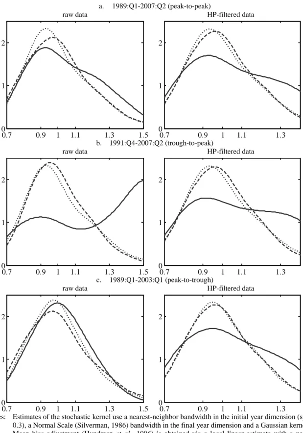
convergence dynamics using both raw and HP-filtered data. Drawing on Magrini et al. (2013), the expectation is that, if the filtering procedure does not spuriously modify convergence dynamics, substantially the same result should be found using both raw and HP-filtered data over sub-periods stretching between two corresponding points along the cycle (e.g., a peak-to-peak sub-period). In addition, given that disparities follow a pro-cyclical behavior in these years (Duran, 2014), we expect the dynamics estimated from raw data to be biased against convergence when a slowdown phase is removed (e.g., a trough-to-peak period), and towards convergence when an expansion is removed (e.g., a peak-to-trough sub-period). In contrast, we expect the results from HP filtered data to be substantially the same over the different sub-periods.

In particular, we focus on the following three sub-periods defined using the US cycle as a reference:

a. a peak-to-peak sub-period – from the peak of 1989:Q1 to the peak of 2007:Q2 b. a trough-to-peak sub-period – from the trough of 1991:Q4 to the peak of 2007:Q2 c. a peak-to-trough sub-period – from the peak of 1989:Q1 to the trough of 2003:Q1

Estimated dynamics are reported in Figure 1. Specifically, panel a refers to the peak-to-peak sub-period, panel b to the trough-to-peak sub-period and panel c to the peak-to-trough one. Each panel then reports the estimate of the cross-sectional distribution at the beginning of the period (the dashed line), at the end of the period (the dotted line) and the estimate of the ergodic distribution (the solid line), for both raw and HP-filtered data.

(14)

13

Concentrating first on the top panel, the comparison between initial, final and ergodic distributions estimated from raw data indicates a tendency towards divergence due to the emergence of a second mode in correspondence to a value of 20-30 percent in excess of the sample mean. In line with expectations, the same type of conclusions can be drawn from the distributions estimated using HP-filtered data thus showing that the filtering procedure has not modified the estimated distribution dynamics with respect to the peak-to-peak sub-period.

Moving then to the other two sub-periods, estimates obtained from raw data clearly confirm that short-run dynamics might strongly affect the results: the removal of a slowdown indeed induces a sizeable bias towards divergence (left hand side of Figure 1, panel b), while the removal of an expansion produces a bias in the opposite direction (left hand side of Figure 1, panel c). Finally, distributions estimated from HP-filtered data over incomplete business cycles (right hand side of Figure 1, panels b and c) point to the same result obtained using the peak-to-peak period (right hand side of Figure 1, panel a).

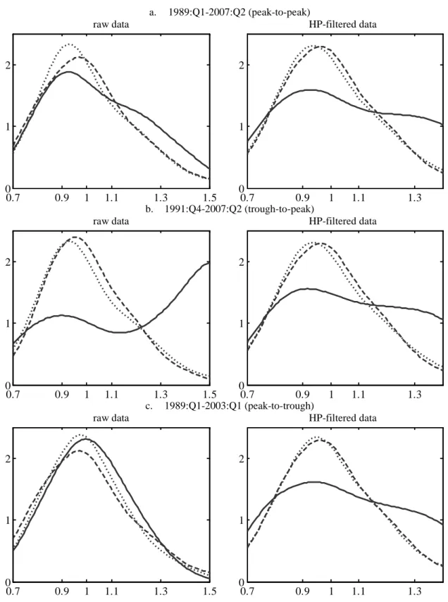
All in all, we believe that these estimates clearly demonstrate the ability of the proposed methodology to provide unbiased results, even when the analyzed period does not coincide with (at least) one complete cycle. However, in order to check the robustness of this result to the choice of the HP parameter, we have also employed the values of 4000, corresponding to the original proportion implicit in Hodrick and Prescott’s choice, and of 20000, implied by a proportion of 3 between average and cut-out cycles. Results obtained using these values are reported in Appendix 1 (Figures A1.1 and A1.2) and clearly confirm the just reached conclusion. However, despite the fact that the estimated distributions tell the same story, the bias appears not to have been completely removed in case λ is set to the value of 4000. This reinforces the principle expressed in Section 2 that the HP parameter must be chosen with

(15)

14

great care in order to ensure that all cyclical swings are actually removed.

3.2 Annual data

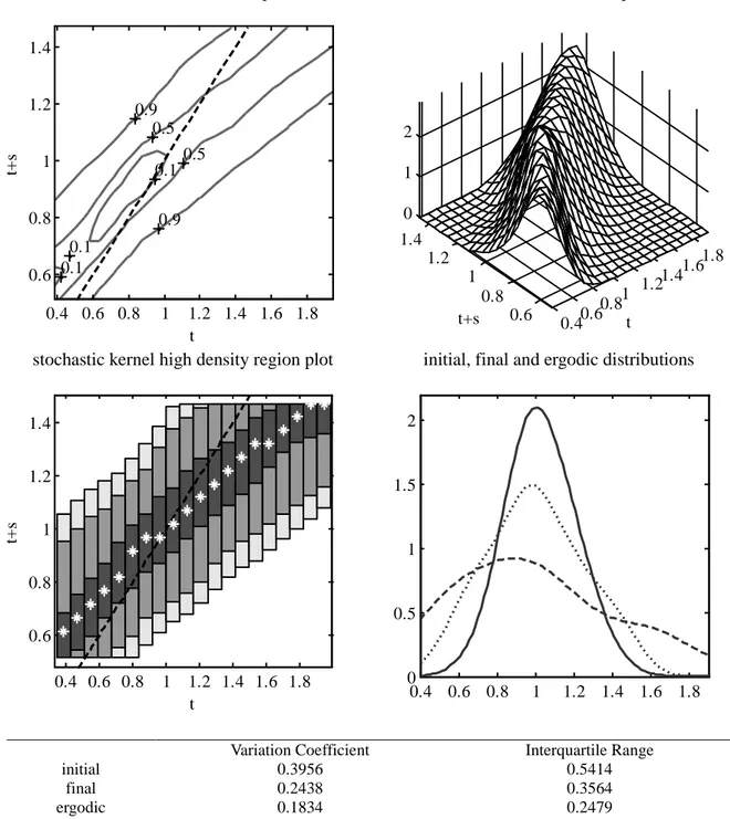
It is now possible to move to the main purpose of this section and, exploiting the larger time span of the annual dataset,4 study convergence dynamics over the entire period running between 1930 and 20105 and in selected sub-periods. In each of the considered cases, attention is primarily focused on the visual inspection of the stochastic kernel estimates and on the differences in the shapes of estimated initial, final and ergodic distributions. In addition, the evidence provided by the graph is supported by a comparison between dispersion indexes such as the variation coefficient and the interquartile range.

The estimate of the probability mass reported in Figure 2 clearly displays an ample clockwise rotation with respect to the main diagonal, thus indicating the existence of a strong tendency towards convergence for the 48 conterminous states over the entire period. This is clearly confirmed by the fact that the estimated ergodic distribution is considerably more sharply peaked than the distribution estimated for the initial year as well as by the substantial reduction in the two indexes of dispersion.

(Figure 2 around here)

Behind these dynamics it is however possible to identify three distinct phases. The first is a

4 _{Preliminarily, we confirm that the methodology is actually characterised by the same degree of efficacy also}

when annual data are employed. In Figure A1.3 we compare the estimated distribution dynamics using both datasets over the same time period. To allow for the endpoints problem described in Section 2, the analysis is carried out over the period 1971:Q1-2010:Q4 using quarterly data, and between 1971 and 2010 using annual data. The shape of the estimated distributions is essentially identical, confirming that the answer provided by the proposed methodology over the same period is unaltered, independently of the frequency of the data. Incidentally, the considered period appears to be characterized by a weak tendency towards divergence.

5_{In this case, the sample endpoint estimated values excluded from the analysis are 2, one at each side of the}

(16)

15

phase of very strong convergence that runs from 1930 to 1970. As is often customary, we have divided this period into two sub-periods, separated by the end of WWII. Thus, Figure 3 depicts the strong tendency towards convergence experienced between 1930 and 1945 and the same dynamic is then found in the period 1946-1970 displayed in Figure 4. In both cases there is indeed a noticeable clockwise rotation of the estimated probability mass and a sharply concentrated unimodal ergodic distribution.

(Figures 3 and 4 around here)

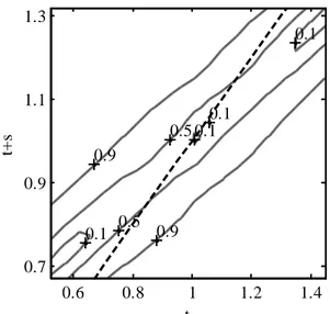
A phase of substantial persistence instead characterizes the period around the oil shocks (1971-1980). This is illustrated in Figure 5. Here, the probability lays over the main diagonal thus indicating a tendency for the states not to exchange their positions within the distribution. By the same token, the shape of the ergodic distribution is very similar to those corresponding to the initial and final years and the dispersion indexes remain substantially unaltered.

(Figure 5 around here)

The period that starts with the 1980’s witnesses a radical change in the dynamics with a switch towards divergence. Figure 6, that refers to the 1981-2010 period, exhibits a twist of the conditional probability mass, with an evident anti-clockwise rotation for values of per capita personal income in excess of 110 percent of the sample average at the beginning of the period. Consistently, the estimated ergodic distribution manifests a sharp increase in dispersion and a strong tendency towards bimodality.

(17)

16

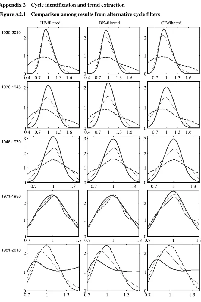
As anticipated, we also perform a robustness check by replicating the analysis based on the annual dataset using BK and CF filters. For each of them, the cut-out frequency has been selected in accordance with the choice of λ described in detail in Section 2.1. The estimates obtained with the alternative filters are summarized in Appendix 2 (Figure A2.1) and clearly confirm the previously reported findings.

3.3 Spatial dependence

A possibly critical issue within the distribution dynamics approach concerns the effects of spatial dependence on the kernel density estimates. While in the literature on convergence within the regression approach there is a full awareness that neglecting spatial dependence may lead to biased and inefficient estimates, this issue has so far received much less attention within the nonparametric literature.

Typically, in the distribution dynamics framework, the issue is tackled by adopting a spatial filtering technique before proceeding with the estimate of the stochastic kernel. For example, Basile (2010) fits a spatial autoregressive model and employs residuals for subsequent analysis while Fischer and Stumpner (2008) and Maza et al. (2010) employ a filtering approach based on the local spatial autocorrelation statistic Gi developed by Getis and Ord (1992). Underlying this way of approaching the issue there is a strict assumption: spatial dependence is seen as a nuisance element that should be excluded in order to avoid the risk of losing the statistical properties of the estimates (Anselin 2002, 2009). It must be recognized, however, that spatial dependence might alternatively be a substantive element of the process under study. Rey (2001), for instance, notes that the intra-distribution mobility of the US states is significantly affected by the relative position of neighbors within the cross-sectional

(18)

17

distribution of income. In such instances, spatial dependence embodies valuable information on convergence dynamics and adopting a spatial filtering technique appears a controversial strategy (Magrini, 2004) as it may yield misleading results. Nevertheless, as a further check of the robustness the results, we replicate the analysis using data which have been previously spatially filtered by fitting a spatial autoregressive model. The outcomes are in Appendix 3. The evolution of the Morans’s I index values (all statistically significant at the 1 percent level) is reported in Figure A3.1, manifesting a behavior in line with Rey and Montouri (1999). The distributions estimated using spatially filtered data are depicted in Figure A3.2. and clearly confirm the results obtained from un-filtered data.

4 Conclusions

When regional disparities follow a distinct cyclical pattern in the short-run, convergence analysis should be carried out with great care to avoid distortions in the results. Indeed, Magrini et al. (2013) have shown that these distortions could be quite sizeable when convergence is analyzed over a period that includes incomplete cycles. Here, we tackle this issue by proposing an approach that identifies long-term dynamics of the cross-section distribution of per capita income by filtering away short-term, business cycle-related fluctuations from regional time series.

Our approach has two main advantages: firstly, it allows to unbiasedly analyze convergence over any possible period rather than over periods rigidly determined by turning points (as in Magrini et al., 2013); secondly, it avoids distorted results even when the nature of the cyclical pattern changes over time. Coupling this approach with a continuous state-space distribution dynamics method, we analyze convergence across 48 conterminous US states between 1930 and 2010 and report a strong tendency towards convergence up to the beginning of the 1970s

(19)

18

followed, from the beginning of the 1980s, by a phase of sizeable divergence.

Incidentally, we note that this shift from a convergence to a divergence pattern appears to parallel the shift from the “Great Compression” to the “Great Divergence” envisaged by Krugman (2007) with respect to the distribution of income across individuals within the US. This may suggest that similar causes that have led to an increase in income disparities across individuals might have also contributed to sustaining the gap between richer and poorer areas of the nation. In fact, this would not be really surprising: disparities in per capita income levels within the society, from the best paid higher managers and professionals to the worst remunerated unskilled worker, have a spatial manifestation due to location decisions and the tendency for people to live close to people like themselves. Therefore, changes in the societal dimension of income distribution naturally lead to changes in the distribution of income across areas.

There is an heated debate with respect to the interpretation of the societal dimension of the disparities, to the identification of its causes and to the prescription of policy interventions. Independently of the position in this debate, a further aspect should be considered explicitly: building on this societal dimension of disparities, there is a danger that a truly spatial dimension may develop. Such a spatial dimension can be seen as the combined result of adjustment costs through space, rigidities and endogenous dynamics of local development factors and agglomeration. These dynamics can indeed determine a spatially non-homogenous equilibrium distribution of per capita income since they shape disparities across regions in the sectoral structure of the economies, in the transmission of signals among firms (related to localization and urbanization externalities), in the education system, local entrepreneurial capacity, risk capital, local labor markets’ matching efficiency and in the structure of this

(20)

19

mismatch. The end result is the increase in the risk that that life opportunities of otherwise similar people, born in poor or rich regions, will be substantially different and this may naturally contribute to the decline in social mobility described in Levine (2012).

(21)

20

References

Abreu, M., de Groot, H.L.F. and R.J.G.M. Florax. 2005. “Space and Growth: a Survey of Empirical Evidence and Methods.” Région and Développement 21(1): 13–44.

Anselin, L. 2002. “Under the hood: Issues in the Specification and Interpretation of Spatial Regression Models.” Agricultural Economics 27(3): 247–267.

Anselin, L. 2009. “Spatial Regression.” In The SAGE Handbook of Spatial Analysis, edited by Fotheringham, A.S. and P.A. Rogerson, 255–276. London: SAGE.

Barro, R.J. and X. Sala-i-Martin. 1991. “Convergence across States and Regions.” Brooking Papers on Economic Activity 1: 107–182.

Barro, R.J. and X. Sala-i-Martin. 1992. “Convergence.” Journal of Political Economy 100(2): 223–251.

Barro, R.J. and X. Sala-i-Martin. 1995. Economic Growth. New York: McGraw-Hill.

Basile, R. 2010. “Intra-Distribution Dynamics of Regional per-capita Income in Europe: Evidence from Alternative Conditional Density Estimators.” Statistica, Department of Statistics, University of Bologna, vol. 70(1): 3–22.

Baxter, M. and R.G. King. 1999. “Measuring Business Cycles: Approximate Bandpass Filters.” The Review of Economics and Statistics 81(4): 575–593.

Canova, F. 1998. “Detrending and Business Cycle Facts.” Journal of Monetary Economics 41(3): 475–512.

Checherita, C.D. 2009. “Variations on Economic Convergence: the Case of the United States.” Papers in Regional Science 88(2): 259–278.

Christiano, L.J. and T.J. Fitzgerald, 1999. “The Band Pass Filter.” NBER Working Paper 7257, Cambridge, MA: National Bureau of Economic Research.

Christiano, L.J. and T.J. Fitzgerald, 2003. “The Band Pass Filter.” International Economic Review 44(2): 435–465.

(22)

21

DiCecio, R. and C. Gascon. 2010. “Income Convergence in the United States: A Tale of Migration and Urbanization.” The Annals of Regional Science 45(2): 365–377.

Duran, E.H. 2014. “Short Run Dynamics of Income Disparities and Regional Cycle Synchronization in the U.S.” Growth and Change (forthcoming).

Durlauf, S.N. and D.T. Quah. 1999. “The New Empirics of Economic Growth.” In Handbook of Macroeconomics, edited by Taylor, J. and M. Woodford, 235–308. Amsterdam: Elsevier. Durlauf, S.N., Johnson, P.A. and J.R.W. Temple. 2005. “Growth Econometrics.” In Handbook of Economic Growth, edited by Aghion, P. and S.N. Durlauf, 555–677. Amsterdam: Elsevier. Fischer, M.M. and P. Stumpner. 2008. “Income Distribution Dynamics and Cross-Region Convergence in Europe. Spatial Filtering and Novel Stochastic Kernel Representations.” Journal of Geographical Systems 10(2): 109-140.

Garofalo, G.A. and S. Yamarik. 2002. “Regional Convergence: Evidence from a New State-by-State Capital Stock Series.” Review of Economics and Statistics 84(2): 316–323.

Garratt, A., Lee, K., Mise, E and K. Shields. 2008. “Real-Time Representations of the Output Gap.” The Review of Economics and Statistics 90(4): 792–804.

Getis, A. and J.K. Ord. 1992. “The Analysis of Spatial Association by Use of Distance Statistics.” Geographical Analysis 24(3):189–206.

Gomez, V. 2001. “The Use of Butterworth Filters for Trend and Cycle Estimation in Economic Time Series.” Journal of Business and Economic Statistics 19(3): 365–373.

Hammond, G.W. and E. Thompson. 2002. “Mobility and Modality Trends in US State Personal Income.” Regional Studies 36(4): 375–387.

Harvey, A. and T. Trimbur. 2008. “Trend Estimation and the Hodrick-Prescott Filter.” Journal of the Japan Statistical Society 38(1): 41–49.

Hierro, M. and A. Maza. 2009. “Non-stationary Transition Matrices: An Overlooked Issue in Intra-distribution Dynamics.” Economic Letters 103(2): 107–109.

(23)

22

Higgins, M.J., Levy, D. and A.T. Young. 2006. “Growth and Convergence across the United States: Evidence from County-Level Data.” The Review of Economics and Statistics 88(4): 671–681.

Hodrick, R. and E.C. Prescott. 1997. “Postwar U.S. Business Cycles: An Empirical Investigation.” Journal of Money, Credit and Banking 29(1): 1–16.

Holmes, M.J., Otero, J. and T. Panagiotidis. 2013. “A Note on the Extent of U.S. Regional Income Convergence.” Macroeconomic Dynamics (forthcoming).

Hyndman, R.J. 1996. “Computing and Graphing Highest Density Regions.” The American Statistician 50(4) 120-126.

Hyndman, R.J., Bashtannyk, D.M. and G.K. Grunwald. 1996. “Estimating and Visualizing Conditional Densities.” Journal of Computational and Graphical Statistics 5(4): 315–336. Islam, N. 2003. “What Have We Learnt from the Convergence Debate?” Journal of Economic Surveys 17(3): 309–362.

Johnson, P.A. 2000. “A Nonparametric Analysis of Income Convergence across the US States.” Economics Letters 69(2): 219–223.

Kaiser, R. and A. Maravall. 1999. “Estimation of the Business Cycle: A Modified Hodrick-Prescott Filter.” Spanish Economic Review 1(2): 175–206.

Kaiser, R. and A. Maravall. 2001. Measuring Business Cycles in Economic Time Series, Lecture Notes in Statistics 154. New York: Springer-Verlag.

Kane, R. 2001. “Investigating Convergence of the U.S. Regions: A Time-Series Analysis.” Journal of Regional Analysis and Policy 31(1): 1–22.

Krugman, P. 2007. The Conscience of a Liberal. New York: Norton.

Lall, S. and S. Yilmaz. 2001. “Regional Economic Convergence: Do Policy Instruments Make a Difference?” Annals of Regional Science 35(1): 153–166.

(24)

23

Levine, L. 2012. “The US Income Distribution and Mobility: Trends and International Comparisons.” Congressional Research Service Report R42400. Washington, DC: Congressional Research Service.

Loader, C. 1999. Local Regression and Likelihood. New York: Springer.

Magrini, S. 1999. “The Evolution of Income Disparities Among the Regions of the European Union.” Regional Science and Urban Economics 29(2): 257–281.

Magrini, S. 2004. “Regional (Di)Convergence.” In Handbook of Regional and Urban Economics, edited by Henderson, J.V. and J.-F. Thisse, 2741–2796. Amsterdam: Elsevier. Magrini, S. 2009. “Why Should We Analyse Convergence Using the Distribution Dynamics Approach?” Scienze Regionali – Italian Journal of Regional Science 8(1): 5–34.

Magrini, S., Gerolimetto, M. and H.E. Duran. 2013. “Regional Convergence and Aggregate Business Cycle in the United States.” Regional Studies (forthcoming).

Marcet, A. and M. Ravn. 2004. “The HP-Filter in Cross-Country Comparisons.” CEPR discussion paper 4244. London: Centre for Economic Policy Research.

Maza, A., Hierro, M. and J. Villaverde. 2010. “Measuring Intra-Distribution Dynamics: An Application of Different Approaches to the European Regions.” Annals of Regional Science 45(2): 313-329.

Mello, M. 2011. “Stochastic Convergence across US States.” Macroeconomic Dynamics 15(2): 160–183.

Miller, J.R. and I. Genc. 2005. “Alternative Regional Specification and Convergence of U.S. Regional Growth Rates.” The Annals of Regional Science 39(2): 241–252.

Mise, E., Tae-Hwan, K. and P. Newbold. 2005. “On Suboptimality of the Hodrick–Prescott Filter at Time Series Endpoints.” Journal of Macroeconomics 27(1): 53–67.

Paige, R.L. and A.A. Trindade. 2010. “The Hodrick-Prescott Filter: A Special Case of Penalized Spline Smoothing.” Electronic Journal of Statistics 4: 856–874.

(25)

24

Papyrakis, E. and R. Gerlagh. 2007. “Resource Abundance and Economic Growth in the United States.” European Economic Review 51(4): 1011–1039.

Pedersen, T.M. 2001. “The Hodrick-Prescott Filter, the Slutzky Effect, and the Distortionary Effect of Filters.” Journal of Economic Dynamics and Control 25(8): 1081–1101.

Pekkala, S. 2000. “Aggregate Economic Fluctuations and Regional Convergence: The Finnish Case, 1988–1995.” Applied Economics 32(2): 211–219.

Petrakos, G., Rodríguez-Pose, A. and A. Rovolis. 2005. “Growth, Integration, and Regional Disparities in the European Union.” Environment and Planning A 37(10), 1837–1857.

Quah, D.T. 1993a. “Empirical Cross-Section Dynamics in Economic Growth.” European Economic Review 37(2-3): 426–434.

Quah, D.T. 1993b. “Galton’s Fallacy and Tests of the Convergence Hypothesis.” Scandinavian Journal of Economics 95(4): 427–443.

Quah, D.T. 1996a. “Empirics for Economic Growth and Convergence.” European Economic Review 40(6): 1353–1375.

Quah, D.T. 1996b. “Convergence Empirics across Economies with (Some) Capital Mobility.” Journal of Economic Growth 1(1): 95–124.

Quah, D.T. 1997. “Empirics for Growth and Distribution: Stratification, Polarization, and Convergence Clubs.” Journal of Economic Growth 2(1): 27–59.

Ravn, M.O. and H. Uhlig. 2002. “On Adjusting the Hodrick-Prescott Filter for the Frequency of Observations.” The Review of Economics and Statistics 84(2): 371–380.

Rey, S.J. 2001. “Spatial Empirics for Economic Growth and Convergence.” Geographical Analysis 33(3), 195-214.

Rey, S.J. and B.D. Montouri. “US Regional Income Convergence: A Spatial Econometric Perspective.” Regional Studies 33(2): 143–156.

(26)

25

Shioji, E. 2001. “Public Capital and Economic Growth: A Convergence Approach.” Journal of Economic Growth 6(3): 205–227.

Silverman, B.W. 1986. Density Estimation for Statistics and Data Analysis. London: Chapman & Hall.

Solow, R.M. 1956. “A Contribution to the Theory of Economic Growth.” Quarterly Journal of Economics 70(1): 65–94.

Swan, T.W. 1956. “Economic Growth and Capital Accumulation.” Economic Review 32(2): 334–361.

Temple, J. 1999. “The New Growth Evidence.” Journal of Economic Literature 37(1): 112– 156.

Tomljanovich, M. and T.J. Vogelsang. 2001. “Are U.S. Regions Converging? Using New Econometric Methods to Examine Old Issues.” Empirical Economics 27(1): 49–62.

Wang, Y. 2004. “A Nonparametric Analysis of the Personal Income Distribution across the Provinces and States in the U.S. and Canada.” Regional and Sectoral Economic Studies 4(1): 5–24.

Yamamoto, D. 2008. “Scales of Regional Income Disparities in the USA, 1955-2003.” Journal of Economic Geography 8(1): 79–103.

Yu, C. 2012. “The Evolution of U.S. Regional Inequality: A Mixture Model Explanatory Approach.” REAL discussion paper 12-T-04. Urbana-Champaign, IL: Regional Economics Application Laboratory.

Yu, J. and L.-F. Lee. 2012. “Convergence: A Spatial Dynamic Panel Data Approach.” Global Journal of Economics 1(1): 1–36.

Zarnowitz, V. and A. Ozyildirim. 2006. “Time Series Decomposition and Measurement of Business Cycles, Trends and Growth Cycles.” Journal of Monetary Economics 53(7): 1717– 1739.

(27)

26

Figure 1 Comparison between raw and HP-filtered data

a. 1989:Q1-2007:Q2 (peak-to-peak)

raw data HP-filtered data

b. 1991:Q4-2007:Q2 (trough-to-peak)

c. 1989:Q1-2003:Q1 (peak-to-trough)

Notes: Estimates of the stochastic kernel use a nearest-neighbor bandwidth in the initial year dimension (span = 0.3), a Normal Scale (Silverman, 1986) bandwidth in the final year dimension and a Gaussian kernel. Mean bias adjustment (Hyndman et al., 1996) is obtained via a local linear estimate with a nearest-neighbor bandwidth (with span chosen to minimize AIC).

HP-filtered data are obtained setting λ = 10000.

The dashed line represents the initial year, the dotted line represents the final year, the continuous line represents the ergodic.

0.7 0.9 1 1.1 1.3 1.5 0 1 2 0.7 0.9 1 1.1 1.3 0 1 2 0.7 0.9 1 1.1 1.3 1.5 0 1 2 0.7 0.9 1 1.1 1.3 0 1 2 0.7 0.9 1 1.1 1.3 1.5 0 1 2 0.7 0.9 1 1.1 1.3 0 1 2

(28)

27

Figure 2 annual data: 1930-2010

stochastic kernel contour plot stochastic kernel 3D plot

stochastic kernel high density region plot initial, final and ergodic distributions

Variation Coefficient Interquartile Range

initial 0.3956 0.5414

final 0.1807 0.2519

ergodic 0.1642 0.2160

In contour and HDR plots, the dashed line represents the main diagonal, the asterisk the modes. In the comparison between distributions, the dashed line represents the initial year, the dotted line represents the final year, the continuous line represents the ergodic.

0.9 0.9 0.5 0.5 0.1 0.1 t t+ s 0.4 0.6 0.8 1 1.2 1.4 1.6 1.8 0.8 1 1.2 1.4 0.40.6 0.81 1.21.4 1.61.8 0.8 1 1.2 1.4 0 1 2 3 t t+s 0.4 0.6 0.8 1 1.2 1.4 1.6 1.8 0.8 1 1.2 1.4 t t+ s 0.4 0.6 0.8 1 1.2 1.4 1.6 1.8 0 0.5 1 1.5 2 2.5

(29)

28

initial 0.3956 0.5414

final 0.2438 0.3564

ergodic 0.1834 0.2479

0.9 0.9 0.5 0.5 0.1 0.1 0.1 t t+ s 0.4 0.6 0.8 1 1.2 1.4 1.6 1.8 0.6 0.8 1 1.2 1.4 0.40.6 0.81 1.21.4 1.61.8 0.6 0.8 1 1.2 1.4 0 1 2 t t+s 0.4 0.6 0.8 1 1.2 1.4 1.6 1.8 0.6 0.8 1 1.2 1.4 t t+ s 0.4 0.6 0.8 1 1.2 1.4 1.6 1.8 0 0.5 1 1.5 2

(30)

29

initial 0.2345 0.3396

final 0.1589 0.1947

ergodic 0.1266 0.1664

0.9 0.9 0.5 0.5 0.1 0.1 0.1 0.1 t t+ s 0.6 0.8 1 1.2 1.4 0.7 0.9 1.1 1.3 0.6 0.8 1 1.2 1.4 0.7 0.9 1.1 1.3 0 2 4 t t+s 0.6 0.8 1 1.2 1.4 0.7 0.9 1.1 1.3 t t+ s 0.6 0.8 1 1.2 1.4 0 0.5 1 1.5 2 2.5 3

(31)

30

initial 0.1537 0.1887

final 0.1416 0.1990

ergodic 0.1428 0.2054

0.9 0.9 0.5 0.5 0.1 0.10.1 0.1 t t+ s 0.7 0.9 1.1 1.3 0.8 1 1.2 0.7 0.9 1.1 1.3 0.8 1 1.2 0 2 4 t t+s 0.7 0.9 1.1 1.3 0.8 1 1.2 t t+ s 0.7 0.9 1.1 1.3 0 0.5 1 1.5 2 2.5

(32)

31

initial 0.1437 0.2214

final 0.1807 0.2519

ergodic 0.2188 0.4069

0.9 0.9 0.5 0.5 0.1 0.10.1 t t+ s 0.7 0.9 1.1 1.3 0.8 1 1.2 1.4 0.7 0.9 1.1 1.3 0.8 1 1.2 1.4 0 1 2 3 t t+s 0.7 0.9 1.1 1.3 0.8 1 1.2 1.4 t t+ s 0.7 0.9 1.1 1.3 1.5 0 0.5 1 1.5 2 2.5

(33)

32

Appendix 1 Check of the methodology

Figure A1.1 Comparison between raw and HP-filtered data (λ = 4000)

a. 1989:Q1-2007:Q2 (peak-to-peak)

0.7 0.9 1 1.1 1.3 1.5 0 1 2 0.7 0.9 1 1.1 1.3 0 1 2 0.7 0.9 1 1.1 1.3 1.5 0 1 2 0.7 0.9 1 1.1 1.3 0 1 2 0.7 0.9 1 1.1 1.3 1.5 0 1 2 0.7 0.9 1 1.1 1.3 0 1 2

(34)

33

Figure A1.2 Comparison between raw and HP-filtered data (λ = 20000)

a. 1989:Q1-2007:Q2 (peak-to-peak)

0.7 0.9 1 1.1 1.3 1.5 0 1 2 0.7 0.9 1 1.1 1.3 0 1 2 0.7 0.9 1 1.1 1.3 1.5 0 1 2 0.7 0.9 1 1.1 1.3 0 1 2 0.7 0.9 1 1.1 1.3 1.5 0 1 2 0.7 0.9 1 1.1 1.3 0 1 2

(35)

34

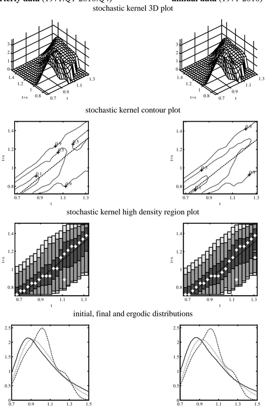
Figure A1.3 comparison between results from quarterly and annual data, 1971 -2010 quarterly data (1971:Q1-2010:Q4) annual data (1971-2010)

stochastic kernel 3D plot

stochastic kernel contour plot

stochastic kernel high density region plot

initial, final and ergodic distributions

HP-filtered data are obtained setting λ = 10000 for quarterly data and λ = 40 for annual data.

0.7 0.9 1.1 1.3 0.8 1 1.2 1.4 0 1 2 3 t t+s 0.7 0.9 1.1 1.3 0.8 1 1.2 1.4 0 1 2 3 t t+s 0.9 0.9 0.5 0.5 0.1 t t+ s 0.7 0.9 1.1 1.3 0.8 1 1.2 1.4 0.9 0.9 0.5 0.1 t t+ s 0.7 0.9 1.1 1.3 0.8 1 1.2 1.4 0.7 0.9 1.1 1.3 0.8 1 1.2 1.4 t t+ s 0.7 0.9 1.1 1.3 0.8 1 1.2 1.4 t t+ s 0.7 0.9 1.1 1.3 1.5 0 0.5 1 1.5 2 2.5 0.7 0.9 1.1 1.3 1.5 0 0.5 1 1.5 2 2.5

(36)

35

Appendix 2 Cycle identification and trend extraction

Figure A2.1 Comparison among results from alternative cycle filters

HP-filtered BK-filtered CF-filtered

1930-2010

1930-1945

1946-1970

1971-1980

1981-2010

Notes: HP-filtered data are obtained setting λ = 40. Correspondingly, BK-filter and CF-filter identify the trend by removing components whose frequency is lower than 16. The number of leads and lags in the BK-filter is equal to 3. 0.4 0.7 1 1.3 1.6 0 1 2 0.4 0.7 1 1.3 1.6 0 1 2 0.7 1 1.3 1.6 0 1 2 0.4 0.7 1 1.3 1.6 0 1 2 0.4 0.7 1 1.3 1.6 0 1 2 0.7 1 1.3 1.6 0 1 2 0.7 1 1.3 0 1 2 3 0.7 1 1.3 0 1 2 3 0.7 1 1.3 0 1 2 3 0.7 1 1.3 0 1 2 0.7 1 1.3 0 1 2 0.7 1 1.3 0 1 2 0.7 1 1.3 0 1 2 0.7 1 1.3 0 1 2 0.7 1 1.3 0 1 2

(37)

36

Appendix 3 Spatial dependence Figure A3.1 Moran’s I index

Notes: The index is calculated using a 6-nearest neighbors spatial weight matrix. In all years, the null hypothesis of independence is rejected at the 1% level.

1920

1940

1960

1980

2000

2020

0.2

0.3

0.4

0.5

0.6

0.7

(38)

37

Figure A3.2 Comparison between results from spatially filtered and unfiltered data

HP-filtered HP-filtered and spatially filtered

1930-2010

1930-1945

1946-1970

1971-1980

1981-2010

Notes: HP-filtered data are obtained setting λ = 40.

Spatially filtered data are the residuals from a spatial autoregressive model using a 6-nearest neighbors spatial weight matrix.

0.4 0.7 1 1.3 1.6 0 1 2 0.7 1 1.3 1.6 0 1 2 0.4 0.7 1 1.3 1.6 0 1 2 0.7 1 1.3 1.6 0 1 2 0.6 0.7 0.8 0.9 1 1.1 1.2 1.3 1.4 0 1 2 3 0.8 0.9 1 1.1 1.2 1.3 0 1 2 3 0.7 0.8 0.9 1 1.1 1.2 1.3 0 1 2 0.8 0.9 1 1.1 1.2 0 1 2 0.7 0.8 0.9 1 1.1 1.2 1.3 1.4 1.5 0 1 2 0.8 0.9 1 1.1 1.2 1.3 0 1 2