from Italy’s Unification
to the Single European Currency
Franco Spinelli* and Carmine Trecroci**
*University of Brescia
**University of Brescia and University of Glasgow
This article analyses the behaviour of several price indexes over the whole life of the Italian lira (1861-1998), and for various sub-periods defined by the exchange-rate regimes of the Italian monetary history. We focus on the persistence and stationarity properties of the inflation process and their dependence on the real cycle. An international comparison with the United States and the United Kingdom further supports the conclusion that Italian inflation was abnormal as far as its mean value, degree of persistence and relationship to the real cycle are concerned. In particular, we find that the output-inflation relationship had a textbook-like, positive slope only during periods of low inflation and low production volatility.
1. Introduction
With the worldwide decrease of inflation rates over the past 25 years and, in the case of Europe, following the changeover to the single currency and the establishment of the Eurosystem, the origins and the dynamics of the price variation processes have disappeared from the research agenda, which they had dominated in the previous three decades.
This is unsatisfactory for several reasons. First, there is still a great deal we do not know about inflationary processes. Second, in the past there have been several instances where inflation was particularly low and dependent on exogenous factors, and they can help us interpret the current state of affairs. Third, inflation has never fully disappeared, and the ultimate defence against a return to high inflation does not lie only in monetary constitutionalism or in the independence of central
1 The sources and the construction methods regarding the different indexes are
available in Micheletti and Spinelli (2001).
banks. It probably lies in the mental attitude of the public at large towards it and in the diffuse knowledge that economists disseminate outside the scientific community. It is therefore compelling to provide a rigorous analysis of this phenomenon, but one which possibly shuns strictly technical arguments and tools. These considerations motivate the present study.
Our analysis focuses on the long-run behaviour of the Italian lira’s purchasing power. It mainly employs charts and relatively simple quantitative tests. Several price indexes are examined for the entire period of life of the lira – 1861 to 1998 – as well as for the individual decades and the sub-periods of fixed and floating exchange rates. The final sections extend the analysis to an international comparison with the United States and the United Kingdom, in order to clarify the extent to which the Italian inflationary process is an outlier.
2. The Italian price level from 1861 to 1998
This section introduces to the behaviour of prices over the entire period of life of the lira (1861-1998). A graphical presentation of three price indexes is followed by a statistical analysis of their fluctuations. In particular, we look at mean values, volatility, normality, persistence and stationarity over the whole period, and also study the single decades and sub-periods defined by the different monetary and exchange regimes of the Italian monetary history.
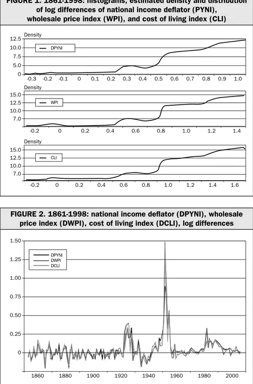
We consider three price indexes: the national income deflator (PYNI), the cost-of-living index (CLI) and the wholesale price index (WPI)1. Figure 1 plots their natural logarithms. Several features emerge. Up until WWII, we notice a limited variability around stable mean values. This period of relative stability is followed by the sizeable inflationary process of WWI and its aftermath. However, between the late 1920s and the end of the 1930s there is a reversal towards a lower price level. This is followed by a second, more marked bout of inflation
that ends in 1947-48. Over the 1950s and early 1970s, the indexes remain stable or rise only slightly. Then, we have a third inflationary process. It differs from the others in two respects: it does not coincide with a war, and it is more gradual, but also more persistent. Indeed, inflation does not return to “normal” values up to the eve of lira’s entry into the EMU, and therefore the end of our sample period.
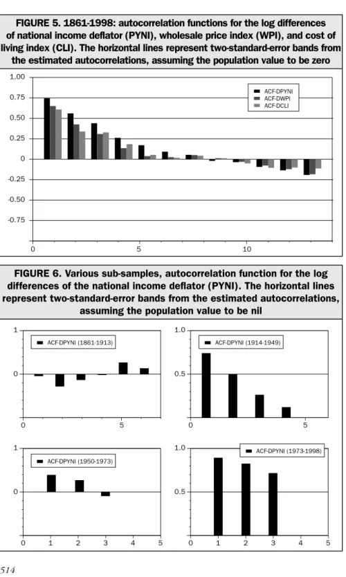
The annual changes depicted in Figure 2 make clearer the differences between the various historical regimes. In particular, a long initial period characterised by sequences of relatively low rates of inflation and deflation is followed by three high-inflation processes and by the interwar years, which present a marked, persistent fall in prices.
Therefore, the simple graphical evidence highlights three interesting and intriguing facts:
i) in the long run, Italian prices have a neat tendency to rise;
ii) in the short run, price levels move in every possible direction and even experience a marked and persistent fall;
iii) WWII acts as a watershed between two different price regimes. The former is characterised by price fluctuations which are at times large, but centred on a stable mean value. The latter witnesses systematic price increases, and therefore denotes strong inflation persistence. So, in statistical terms, the two sub-periods show very different degrees of stationarity and autocorrelation.
3. Statistical analysis
We now turn to the analysis of the mean, volatility, normality, persistence and stationarity of the annual variations of the price indexes. In order to detect possible time variations in the processes, we also consider each decade and the sub-periods defined by the different monetary and exchange regimes identified in Fratianni and Spinelli (2001)2. In particular, we will consider the following sub-samples: 1) 1861-1913: the classical gold standard, with prevalence of fixed
exchange rates;
3The high average inflation of the 1914-1949 years could be attributed solely to the two
wars. The average variation for the years 1920-36 never exceeds 1.5%; volatility, however, remains high.
2) 1914-1949: the World Wars and the inter-war period, when floating exchange rates prevailed;
2.1) 1920-1936: the inter-war period, with both fixed and floating exchange rates;
3) 1950-1973: the Bretton Woods system, hence fixed exchange rates; 4) 1974-1998: floating exchange rates prevailing again in a
fixed-but-adjustable peg context.
For each reference period and each price index, Table 1 displays the average rate of change (μ), the standard deviation (σ) and, for a better comparison of volatility between periods characterized by marked differences in average values, the variation coefficient (cv =
σ/μ).
Over the entire sample period, the indexes show average rates of change that are positive, of the order of 6-7%. The decade 1941-1950 is the one with the highest average change, 36%. The decades of the gold standard display lower mean variations, in some cases even negative. As for the post-WWII years, the ‘70s, the ‘80s and the ‘90s are the decades with the highest inflation, their mean values lying between 7.5% and 13.6%. Last, among the four sub-samples defined by the exchange-rate regimes, the years 1861-1913 and 1914-1949 show, respectively, the lowest (PYNI, 0.65%; CLI, 0.38%; WPI, 0,05%) and the highest mean inflation (PYNI, 15.5%; CLI, 14.90%; WPI, 15.34%).
The variation coefficient indicates that the variability of the inflation process has not stayed constant across the changes that its mean value has witnessed over time. This becomes clear if one were to compare the extreme low and high values of the decades 1921-30 and 1941-50. Such finding strengthens the case for time variation in the inflation process and calls for an examination of its stationarity.
Looking at sub-periods, average inflation turns out to be lower
4Recall that Jarque and Bera’s test are markedly weak in small samples. Doornik and
Hansen’s test is therefore justified in the light of the correction it brings to this bias.
5 We do not present results for the sub-sample 1920-1936 because of its too few
observations.
compare the two fixed-exchange-rate sub-periods, we find that the Bretton Woods years have much higher average inflation and lower volatility than the gold standard years. Therefore, one could argue that Bretton Woods in fact sowed the seeds of the subsequent high and persistent inflation.
As for normality, we subjected the time series to the Jarque and Bera test (1987) (e1) and the Doornik and Hansen test (1994) (e2) to check whether asymmetry and kurtosis are the same as in a normal distribution4. Table 2 lists the results of the tests carried out on the entire sample period: there is evidence against normality. For each definition of inflation, Figures 3 and 4 show the histogram, estimated density and distribution (Figure 3), and cumulated distribution crossed with the normal distribution. Again, there is strong evidence of deviations from the normal distribution, in terms of symmetry and kurtosis, which confirms earlier indications from the normality tests.
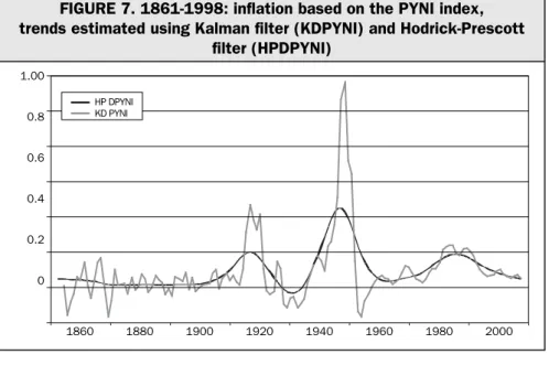
To evaluate persistence, we computed the autocorrelation functions (ACF) up to the tenth lag. The functions, plotted in Figure 5, start with high positive values and then decline fairly regularly; values do not turn negative until the eighth or ninth lag. These are statistically different from zero at least for the first three lags. Therefore, Italian inflation is remarkably persistent.
For the changes in the PYNI index, Figure 6 shows the correlograms centred on the four sub-periods.5Significantly, inflation is more persistent over the floating exchange rate years, and reaches a maximum in the post-Bretton Woods.
Lastly, we examine the processes’ stationarity properties. We employ the standard Augmented Dickey-Fuller (ADF) test, which amounts to evaluating the statistical significance of βin the regression:
Δπt= α+ μτ+ βπt-1+ ∑ n i=1
6The critical values depend on the inclusion of the constant, or of the constant and the
deterministic trend, and are those illustrated in MacKinnon (1991). Significant statistics of 5% are identified by *, and of 1% by **.
7Like most unit root tests, the ADF test has problems connected with a small-sample
bias, or with variables that contain MA components (see for example Maddala and Kim, 1998). However, our results are such to instil reasonable doubt about the constancy of mean and variance properties in the inflation processes.
where (τ) is a deterministic trend. A significant statistic would imply rejection of the the unit root null hypothesis (H0 : β = 0) and hence stationarity of the inflation rate.
Table 3 presents the results of the tests. For completeness, we include the t-values of coefficient βfor both models with constant only, and with constant and trend, each estimated with n = 36.
We summarize the evidence as follows:
a) we reject the null of a unit root in both models at a 1% significance level over the whole sample: inflation appears to be a stationary process;
b) the same applies to the gold standard;
c) on the contrary, the period 1914-1949 is unambiguously characterized by non-stationarity; and
d) for the Bretton Woods years and afterwards, overall results support non-stationarity.
Hence, fixed exchange rates tend to be associated with stationary price changes, whereas floating exchange rates lean towards non-stationarity7. However, the nature and frequency of possible structural changes in the data cannot be determined by means of unit root tests; an explicit treatment of time variation in the basic statistical properties of the variables is called for.
4. Long-term trends and regime changes
Considering the results so far, and the likely presence of structural changes in the data-generating process, it is appropriate to study the long-run properties of inflation in order to discriminate between its permanent and temporary components. We will allow these components
to vary over time in order to account for the apparent variability in the inflation trend over the long run.
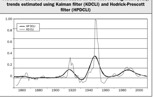
We employ a simple univariate model with unobservable components and stochastic volatility, based on a technique known as Structural Time Series Analysis (STSA), pioneered, among others, by Harvey (1989). The methodology is based on the Kalman filter. For each time series, Figures 7 to 9 plot the estimated trend, along with the one generated by using the more conventional Hodrick-Prescott filter. The main differences between the two estimates lie in the greater volatility of the results obtained with the Kalman filter, and in the general tendency of that trend to adjust to shifts in inflation with some inertia. These are desirable properties of the inflation expectations in that they combine both forward-looking and backward-looking mental processing.
Figure 10 shows the data and the estimated trends for the years from 1949 to 1998. The third great inflation process appears to begin in the early 1960s, to peak in 1978-79, and to return to more moderate levels towards the very end of the period.
5. Inflation and output
In this section, we study the relationship between inflation and output, an issue hotly debated in the past, but which now appears to be only a minor nuisance in research agendas. In our case, the availability of very long time series for output enables to reach sufficiently firm conclusions concerning the cyclical determinants of the inflation process. We analyse the inflation-output relationship according to a largely empirical specification that combines the expectations-augmented Phillips curve (Phelps, 1967; Friedman, 1968) with more recent considerations on persistence and rigidity8(cf. Woodford, 2003).
8 In the 1980s micro and macroeconomic evidence openly contradicted the central
tenets of the New Classical Macroeconomics (NCM). For example, many studies proved that monetary shocks had significant and persistent effects on real output. However, more recent theoretical models recognise the importance of some sort of staggered price-setting mechanism, which implies that fluctuations in output depend on variations in marginal production costs.
The relationship could start from:
πt= ω(yt- yt*) + Et-1πt [1]
where yt- yt*represents the output gap, i.e., the difference between current output level (GDP) and its NAIRU or natural level, and Et-1πtis the expectation of current inflation, formed in the previous period. The dependence of current inflation on information as of the previous period is the result not of the adaptive expectations hypothesis, but of the application of rational expectations to models with a partially rigid price level. All this implies that:
(i) unexpected variations in aggregate demand influence both production and inflation;
(ii) the lower price rigidity, the greater is ω, which represents the slope of the Phillips curve (aggregate supply).
In the literature, we also have the following specification:
πt ω (yt- yt*) + βΕt πt+1 [2]
This differs from the previous equation in that it relates shifts in the curve to variations in current expectations of future inflation. From a theoretical point of view, the two equations are very different; however, because inflation expectations have a high degree of serial correlation, the difference is often elusive on empirical grounds. This is why we adopt the following encompassing model:
πt= ϕΕtπt+1+ ωπt-1γ(yt- yt*) + εt [3] In order to measure the output gap, we extract a stochastic trend from the time series of real GDP; alternatively, we use a trend estimated by means of the Hodrick-Prescott filter, just as we did for expected inflation. Figure 11 shows that, while on the whole the two estimates of the output gap for the period 1861-1998 are similar, at times they present marked differences.
plot of inflation and the output gap, along with a regression line: the negative correlation between inflation and output deviations from its potential is evident. In other words, we uncover a Phillips curve with a positive, non-textbook slope. Since this result is based on a very large sample which includes three intervals of high inflation and consequent structural breaks, it is appropriate to extend the analysis to some sub-samples.
First, we estimate equation [3] with OLS over the entire sample 1861-1998, but with the exclusion of the years 1916-1920 and
1940-1947. The estimates, obtained with PYNI9 and alternatively using the
HP filter and the STSA technique to extract expected inflation and potential output, are as follows (t-value in brackets):
πt= 0.541 Εtπt+1+ 0.268 πt-1+ 0.255 (yt- yt*)HP+ εˆt
(6.13) (3.17) (-1.67)
πt= 0.509 Εtπt+1+ 0.275 πt-1+ 0.092 (yt- yt*)STSA+ εˆt
(5.98) (3.24) (-0.8)
Overall, the output gap turns out to be unimportant for the dynamics of inflation; with the HP filter, it is significant only with a 90% confidence interval. However, the forward-looking expectations regarding current and lagged inflation are significant, and remain so when considering the various sub-samples. As a further validation of the fact that the wide fluctuations in output and inflation essentially drive our results, Figure 13 shows the scatter plots of inflation (DPYNI) and the output gap measures when both the observations concerning the two world wars and the period 1973-1984 are removed from the sample. It is only when major episodes of real output shocks or higher and more persistent inflation are removed from our long sample that the relation between inflation and output gap turns positive.
9The results based on WPI and CLI do not diverge from those obtained with the PYNI,
6. A comparison with the United Kingdom and the United States
It is useful to compare the results concerning Italy with those for other countries over the same period and methodology. We therefore extend the analysis to the United Kingdom and the United States. Figure 14 enables us to make a direct comparison of the dynamics of the GDP deflator of the three countries.
With the exception of the high inflation of the US Civil War, the dynamics looks systematically synchronous. However, Italian inflation clearly has a higher mean value and is more volatile. These differences are quantified in Table 4, which reveals that, for the entire period and each sub-sample except the first, both the mean value and the variability of Italian inflation are higher, often much higher, than for the US and UK. Figure 15 presents the autocorrelation functions of the inflation processes in the three countries. Italy and the United Kingdom denote a similar degree of persistence, which is also much higher than that of the US. Figure 16 shows the autocorrelation functions computed over the four sub-samples: for all countries, but particularly for Italy, inflation shows greater persistence under floating exchange rates.
Moving on to the comparative analysis of the relation between inflation and output gaps, Table 5 presents the results for the US, the UK and Italy of the estimation of the New Keynesian Phillips Curve; the Hodrick-Prescott definition was chosen for the output gap, both for the entire sample and for the three sub-samples – the gold standard, the two world wars and the post-WWII period. The following differences and similarities emerge:
1. When the entire sample is considered, only the UK shows a significant, positive and sizeable output gap coefficient; Italy’s coefficient is negative.
2. As for the sub-samples, output is positively and significantly correlated with inflation in the USA over the periods 1914-1949 and 1950-1998, and in the UK in all the sub-periods except the post-WWII. 3. Inflation expectations prove always and everywhere to be important
4. For all three countries, the gold standard period generates the most ambiguous results.
In short, over periods of low inflation and low macroeconomic volatility, a significant negative trade-off emerges in the US and the UK.
7. Conclusions
The initial graphical analysis, focused on Italy, highlighted the following: a) In the long run, Italian prices tend to rise.
b) On the other hand, in the short run prices display any kind of variation, including a sustained persistent fall, which definitely undermines the idea that there is fundamental downward price rigidity.
c) WWII acts as a watershed between a sub-period of long-term price stationarity and one of persistent inflation.
Moving on to the simple statistical analysis, the mean annual change of Italian price indexes over the entire sample period 1861-1998 turns out to be 6-7%. The decade 1941-1950 has the highest average inflation: 36%. If we consider the sub-periods with fixed and floating exchange rates, the former display a much lower average inflation. Of the two episodes of fixed exchange rates, Bretton Woods suffers from more inflation. Since the Bretton Woods period shows lower volatility too, it might be considered the incubator of the third big inflation, the only one not associated with a war and the most persistent.
Persistence is greater with floating exchange rates, and reaches its maximum in the post-Bretton Woods sub-period.
Formal tests support the conclusion that Italian inflation tends to be stationary under fixed exchange rates and non-stationary under floating rates.
We also look at the relationship between output and inflation. When considering the whole sample, we find a significant negative relation, which implies that supply-side shocks and inflation expectations play a dominant role. The significant positive coefficient that shows up if the two world wars and the post-Bretton Woods years are removed from the sample confirms the above. In a nutshell, the Phillips curve appears only in instances of low inflation and stability of aggregate supply.
When we extend the analysis to the United Kingdom and United States, we find that Italian inflation:
a) is broadly synchronous with those of the other countries; b) presents a much wider volatility;
c) is higher.
The last point is confirmed by the statistical analysis; if we consider the entire sample period, the average annual inflation is 3% for the United Kingdom and only 2.25% for the United States.
Italy proves to be not only the country with the highest average inflation. Compared with inflation in the US and UK, Italian inflation is also the most volatile (13.9% as opposed to 6.30% for the US and 5.75% for UK) and the most persistent, as the study of the autocorrelation functions shows.
Lastly, regarding the relation between output and inflation, the United Kingdom is the only country to have a positive, significant relation for the entire period 1861-1998. For the same period, Italy has a negative significant relation, and the United States a positive insignificant one. This supports the idea that the purchasing power of the Italian lira was indeed the result of the interaction of powerful real shocks which spared the other countries.
REFERENCES
CECCHETTIS.G., HOOPERP., KASMANB.C., SCHOENHOLTZK.L., and WATSONM.W.,
Understanding the Evolving Inflation Process. U.S. Monetary Policy Forum 2007, University of Chicago Graduate School of Business, The
Initiative on Global Financial Markets, 2007.
DOORNIKJ.A. and HANSENH. A Practical Test for Univariate and Multivariate
Normality. Discussion Paper, Nuffield College, 1994.
FRATIANNIM. and SPINELLIF., “Sylos Labini on Fratianni and Spinelli on Inflation:
a Reply”, Banca Nazionale del Lavoro Quarterly Review, 139, 1981, pp. 466-469.
GAROFALOP., Exchange Rate Regimes and Economic Performance: The Italian Experience, Banca d’Italia, Quaderni dell’Ufficio Ricerche Storiche, n. 10,
2005.
JARQUE C.M. and BERA A.K., “A Test for Normalità of Observations and
Regression Residuals”, International Statistical Review, 55, 1987, pp.163-172.
HARVEY A.C., Forecasting, Structural Time Series Models and the Kalman
Filter, Cambridge, CUP, 1989.
KOOPMANS.J., HARVEY A.C., DOORNIKJ.A. and SHEPHARD N., Stamp: Structural
Time Series Analyser, Modeller and Predictor. London, Timberlake
Consultants Press, 2000.
MACKINNON J.G., “Critical Values for Cointegration Tests” in Engle R.F. and
Granger C.W.J. (eds.), Long-run Economic Relationships, Oxford, OUP, 1991, pp. 167-176.
MICHELETTIS. and SPINELLIF., Introduzione all’inflazione italiana: 1861-1998,
Brescia, Edizioni Ori Martin, 2001.
SPINELLI F., I costi dell’instabilità dei prezzi e del cambio. Le analisi delle
Relazioni Annuali della Banca d’Italia: 1894-1998, Milan, Angeli, 2000.
SPINELLIF., “The Determinants of Price and Wage Inflation: the Case of Italy” in
Parkin M. and Zis G. (eds.), Inflation in Open Economies, Manchester, Manchester University Press, 1976, pp. 201-236.
SPINELLI F., “Il dilemma inflazione-disoccupazione: una rilettura critica” in
Rivista Internazionale di Scienze Sociali, LXXXIV, IV-V, 1976, pp. 517-525.
SPINELLIF., “Ancora su inflazione e capacità produttiva: una risposta ad Onori”
in La Malfa G. and Spinelli F., L’economia italiana verso gli anni ’80. VI
Rapporto CEEP, Milan, Angeli, 1980, pp. 77-90.
STOCK J.H. and WATSON M.W., “Why has U.S. Inflation Become Harder to Forecast?”, Journal of Money, Credit and Banking, 2006.
Appendix
The Lira’s Purchasing Power from Italy’s Unification
to the Single European Currency
FIGURE 2. 1861-1998: national income deflator (DPYNI), wholesale price index (DWPI), cost of living index (DCLI), log differences
1.50 1.25 1.00 0.75 0.50 0.25 0 1860 1880 1900 1920 1940 1960 1980 2000 - - - -DPYNI DWPI DCLI
FIGURE 1. 1861-1998: histograms, estimated density and distribution of log differences of national income deflator (PYNI),
wholesale price index (WPI), and cost of living index (CLI)
12.5 10.0 7.5 5.0 0 Density Density DPYNI -0.3 -0.2 -0.1 0 0.1 0.2 0.3 0.4 0.5 0.6 0.7 0.8 0.9 1.0 - - - -15.0 12.5 10.0 7.0 -0.2 0 0.2 0.4 0.6 0.8 1.0 1.2 1.4 - - - -Density 15.0 12.5 10.0 7.0 -0.2 0 0.2 0.4 0.6 0.8 1.0 1.2 1.4 1.6 - - - -WPI CLI
FIGURE 3. 1861-1998: histograms, estimated density and distribution of log differences of national income deflator (PYNI),
wholesale price index (WPI), and cost of living index (CLI)
5.0 2.5 Density Density DPYNI N (s=0.139) -0.3 -0.2 -0.1 0 0.1 0.2 0.3 0.4 0.5 0.6 0.7 0.8 0.9 1.0 - - - -6 4 2 DPYNI N (s=0.17) -0.2 0 0.2 0.4 0.6 0.8 1.0 1.2 1.4 - - - -Density 7.5 5.0 2.5 DPYNI N (s=0.161) -0.2 0 0.2 0.4 0.6 0.8 1.0 1.2 1.4 1.6 - - -
-FIGURE 4. 1861-1998: cumulated distribution of log differences against the normal distribution, for the national income deflator (PYNI),
wholesale price index (WPI), cost of living index (CLI)
1.0 0.5 0 Distribution Distribution DPYNI Normal -0.3 -0.2 -0.1 0 0.1 0.2 0.3 0.4 0.5 0.6 0.7 0.8 0.9 1.0 - - - -2 1 0 -0.2 0 0.2 0.4 0.6 0.8 1.0 1.2 1.4 - - - -Distribution 2 1 0 -0.2 0 0.2 0.4 0.6 0.8 1.0 1.2 1.4 1.6 - - - -DPYNI Normal DPYNI Normal
FIGURE 6. Various sub-samples, autocorrelation function for the log differences of the national income deflator (PYNI). The horizontal lines represent two-standard-error bands from the estimated autocorrelations,
assuming the population value to be nil
1 0 -– - - - - – - -0 5 1.0 0.5 -– – 0 5 1 0 -_ _ _ _ _ _ 0 1 2 3 4 5 1.0 0.5 -_ _ _ _ _ _ 0 1 2 3 4 5 ACF-DPYNI (1861-1913) ACF-DPYNI (1950-1973) ACF-DPYNI (1973-1998) ACF-DPYNI (1914-1949)
FIGURE 5. 1861-1998: autocorrelation functions for the log differences of national income deflator (PYNI), wholesale price index (WPI), and cost of living index (CLI). The horizontal lines represent two-standard-error bands from
the estimated autocorrelations, assuming the population value to be zero
1.00 0.75 0.50 0.25 0 -0.25 -0.50 -0.75 – - - - - – - - - - – - - - -0 5 10 ACF-DPYNI ACF-DWPI ACF-DCLI
FIGURE 7. 1861-1998: inflation based on the PYNI index, trends estimated using Kalman filter (KDPYNI) and Hodrick-Prescott
filter (HPDPYNI) 1.00 0.8 0.6 0.4 0.2 0 1860 1880 1900 1920 1940 1960 1980 2000 - - - -HP DPYNI KD PYNI
FIGURE 8. 1861-1998: inflation based on the wholesale price index (WPI), trends estimated using Kalman filter (KDWPI)
and Hodrick-Prescott filter (HPDWPI)
1.00 0.8 0.6 0.4 0.2 0 1860 1880 1900 1920 1940 1960 1980 2000 - - - -HP DWPI KD WPI
FIGURE 9. 1861-1998: inflation based on the cost-of-living index (CLI), trends estimated using Kalman filter (KDCLI) and Hodrick-Prescott
filter (HPDCLI) 1.00 0.8 0.6 0.4 0.2 0 1860 1880 1900 1920 1940 1960 1980 2000 - - - -HP DCLI KD CLI
FIGURE 10. 1861-1998: inflation based on the PYNI index and trends estimated using Kalman filter and Hodrick-Prescott filter (HPDPYNI)
0.25 0.20 0.15 0.10 0.05 0 -0.05 -0.10 -0.15 1950 1955 1960 1965 1970 1975 1980 1985 1990 1995 2000 - - - -KD PYNI DPYNI HP DPYNI
FIGURE 11. 1949-1998: output gaps, estimated using Kalman filter (KYGAP) and Hodrick-Prescott filter (HPYGAP)
0.4 0.3 0.2 0.1 0 -0.1 -0.2 -0.3 -0.4 1860 1880 1900 1920 1940 1960 1980 2000 - - - -HP YGAP KY GAP
FIGURE 12. 1861-1998: scatter plots of rate of inflation (DPYNI) and output gap, estimated using Kalman
filter and Hodrick-Prescott filter (HPYGAP)
1.0 0.5 0.0 -0.50 -0.45 -0.40 -0.35 -0.30 -0.25 -0.20 -0.15 -0.10 -0.05 0 0.05 0.10 0.15 - - - -HPYGAP DPYNI 1.0 0.5 0.0 -0.30 -0.25 -0.20 -0.15 -0.10 -0.05 0 0.05 0.10 0.15 0.20 0.25 0.30 0.35 0.40 - - - -HPYGAP DPYNI
FIGURE 13. 1861-1915, 1921-1939, 1948-1972, 1985-1998: scatter plots of rate of inflation (DPYNI) and output gap estimated using Kalman filter (KYGAP) and Hodrick-Prescott filter (HPYGAP)
0.1 0 -0.1 -0.050 -0.025 0.0 0.025 0.050 0.075 0.100 0.150 - - - -HPYGAP DPYNI 0.1 0 -0.1 -0.08 -0.06 -0.04 -0.02 0.0 0.02 0.04 0.06 0.08 0.10 0.12 - - - -HPYGAP DPYNI
FIGURE 14. 1861-1998, Italy, USA, UK: rates of inflation
0.8 0.6 0.4 0.2 0 1860 1880 1900 1920 1940 1960 1980 2000 - - - -ITA USA UK
FIGURE 15. 1861-1998, Italy, USA, UK: autocorrelation functions of the inflation rate. Horizontal lines represent two standard deviations bands from estimated autocorrelations, assuming population value to be zero
1.00 0.75 0.50 0.25 0 -0.25 -0.50 -0.75 – - - - - – - - - - – - - - -0 5 10 ACF-ITALY ACF-USA ACF-UK
FIGURE 16. Various sub-samples, Italy, USA, UK. Autocorrelation functions regarding annual variations of deflator of national income. Horizontal lines represent two standard deviation bands from estimated
autocorrelations, assuming population value to be nil
1 0 -– - - - - – - - -0 5 1.0 0.5 -– - - - - – 0 5 1 0 -_ _ _ _ _ _ 0 1 2 3 4 5 1.0 0.5 -_ _ _ _ _ _ 0 1 2 3 4 5 (1861-1913) (1914-1949) (1950-1973) (1973-1998) ITALY USA UK
TABLE 1. National income deflator (PYNI), wholesale price index (WPI), cost of living index (CLI), mean (m), standard deviations (s)
and variation coefficient (cv) of prime differences, various samples
SAMPLE PYNI CLI WPI
cv cv cv 1861-1998 6.805 13.934 2.048 6.448 16.149 2.504 6.029 17.049 2.828 1861-1870 2.015 6.929 3.439 1.877 5.191 2.766 0.100 5.399 53.990 1871-1880 1.178 9.224 7.830 1.619 6.703 4.140 0.528 7.067 13.384 1881-1890 0.000 4.427 NA -0.604 2.876 -4.762 -0.630 4.751 -7.541 1891-1900 0.000 4.519 NA -0.551 0.810 -1.470 -0.360 3.823 -10.619 1901-1910 1.054 4.102 3.892 0.899 2.089 2.324 0.429 3.916 9.128 1911-1920 15.261 13.330 0.873 12.949 13.910 1.074 19.017 16.645 0.875 1921-1930 0.529 7.581 14.331 2.009 7.738 3.852 -3.087 7.597 -2.461 1931-1940 2.773 9.100 3.282 2.069 7.624 3.685 3.064 9.945 3.246 1941-1950 36.496 29.578 0.810 36.837 43.599 1.184 36.946 42.407 1.148 1951-1960 3.058 1.836 0.600 2.435 6.589 2.706 0.575 4.681 8.141 1961-1970 4.421 2.025 0.458 3.807 1.858 0.488 2.573 2.204 0.857 1971-1980 13.614 4.106 0.302 13.128 4.734 0.361 14.283 8.711 0.610 1981-1990 10.034 4.058 0.404 8.730 3.856 0.442 7.418 4.532 0.611 1991-1998 4.349 1.443 0.332 4.155 1.644 0.396 2.934 3.314 1.130 1861-1913 0.647 5.801 8.966 0.382 4.235 11.086 0.047 5.185110.319 1914-1949 15.049 23.252 1.545 14.901 28.602 1.919 15.340 29.416 1.918 1920-1936 1.508 10.976 7.279 1.876 9.566 5.099 -0.873 10.690 -12.245 1950-1973 4.269 2.423 0.568 3.807 2.601 0.683 2.076 4.829 2.326 1974-1998 9.902 5.334 0.539 9.264 5.371 0.580 8.669 7.837 0.904
TABLE 2. 1861-1998: National income deflator (PYNI), wholesale price index (WPI), cost of living index (CLI), mean (m), normality test
on prime differences, 1861-1998 INDEX 1861-1998 e1 e2 ΔPYNI 1375.2* 261.79* ΔCLI 11705.0* 1037.4* ΔWPI 3661.7* 482.95*
TABLE 3. 1861-1998: Augmented Dickey-Fuller Test
PYNI Constant Constant and trend
i=0 i=1 i=2 i=3 i=0 i=1 i=2 i=3
1861-1998 -4.535* -4.095* -3.732* -4.114* -4.656* -4.219* -3.853* -4.285* 1861-1913 -7.364* -6.683* -6.497* -5.662* -7.315* -6.671* -6.512* -5.729* 1914-1949 -2.264 -2.211 -2.082 -2.673 -2.209 -2.171 -2.058 -2.684 1950-1973 -2.004 -1.571 -1.406 -1.154 -2.292 -1.823 -1.807 -1.548 1974-1998 -0.4841 -0.9693 -0.6881 -1.207 -3.719* -3.690* -3.374 -3.582
WPI Constant Constant and trend
i=0 i=1 i=2 i=3 i=0 i=1 i=2 i=3
1861-1998 -5.373* -4.919* -4.229* -4.527* -5.450* -5.006* -4.309* -4.637* 1861-1913 -6.741* -6.421* -6.664* -4.679* -6.725* -6.405* -6.704* -4.742* 1914-1949 -2.758 -2.662 -2.255 -2.758 -2.779 -2.708 -2.299 -2.871 1950-1973 -3.899* -2.544 -2.696 -1.428 -5.068* -4.061* -4.013* -2.979 1974-1998 -2.792 -1.855 -1.325 -1.307 -5.273* -4.522* -3.991* -4.342*
CLI Constant Constant and trend
i=0 i=1 i=2 i=3 i=0 i=1 i=2 i=3
1861-1998 -5.779* -5.501* -3.916* -4.356* -5.893* -5.645* -4.010* -4.494* 1861-1913 -6.299* -5.858* -5.549* -3.828* -6.293* -5.903* -5.643* -3.918* 1914-1949 -3.130* -3.046* -2.088 -2.545 -3.232 -3.211 -2.206 -2.798 1950-1973 -3.595* -2.859 -3.347* -1.667 -3.801* -3.060 -3.362 -1.577 1974-1998 -0.8550 -1.024 -0.8020 -1.261 -4.168* -4.212* -3.942* -4.315*
* Indicates a rejection of the null hypothesis with a 99% confidence inter val.
TABLE 4. USA, UK and Italy, various samples: mean and standard deviation of annual variations of income deflator
YEARS ITALY USA UK
1861-1998 6.805 13.934 2.250 6.313 3.009 5.749 1861-1913 0.647 5.801 0.726 7.560 -0.004 2.310 1914-1949 15.049 23.252 2.308 7.597 3.088 8.255 1920-1936 1.508 10.976 -1.672 7.170 -1.917 7.389 1950-1973 4.269 2.423 3.052 1.785 4.868 2.906 1974-1998 9.902 5.334 4.564 2.433 7.465 4.910
TABLE 5. USA, UK and Italy, various samples: New Keynesian Phillips Curve estimates
NKPC: USA Sample Εtπt+1 πt-1 (yt-yt*)HP 1861-1998 1.031 0.167 0.069 (1.08) (7.16) (2.07) 1861-1913 1.274 -0.042 -0.215 (4.52) (-0.28) (-1.48) 1914-1949 1.285 0.000 0.218 (3.83) (0.00) (1.94) 1950-1998 0.707 0.302 0.127 (6.02) (2.67) (2.16) NKPC: UK Sample Εtπt+1 πt-1 (yt-yt*)HP 1861-1998 0.639 0.397 0.356 (7.04) (5.83) (4.62) 1861-1913 0.331 0.158 0.185 (1.76) (1.15) (1.87) 1914-1949 0.763 0.390 0.463 (2.93) (3.03) (2.79) 1950-1998 0.649 0.369 0.179 (4.90) (2.98) (1.36) NKPC: ITALY Sample Εtπt+1 πt-1 (yt-yt*)HP 1861-1998 0.981 0.079 -0.881 (11.00) (1.09) (-7.55) 1861-1913 0.574 -0.057 -0.383 (1.88) (-0.41) (-1.26) 1914-1949 1.031 0.049 -0.969 (6.07) (0.36) (-4.48) 1950-1998 0.369 0.630 0.023 (3.63) (6.33) (0.178)