Model reduction of stochastic groundwater flow and transport processes

ALMA MATER STUDIORUM - UNIVERSITÀ DI BOLOGNA

Scuola di Dottorato in Ingegneria Civile ed Architettura

Dottorato in Ingegneria Strutturale ed Idraulica, XXV ciclo

08/A1 – ICAR/01

Model reduction of stochastic groundwater

flow and transport processes

Valentina Ciriello

Supervisor:

Coordinator:

Prof. Vittorio Di Federico

Prof. Erasmo Viola

Co-supervisor:

Prof. Alberto Guadagnini

Abstract 7

Sommario 9 1 Introduction 11

Sommario 11 1.1 Uncertainty quantification in modeling ………. 13

1.2 Methodology ………….………. 15

1.3 Research outline ...……….. 17

2 Model reduction strategy 19

Sommario 19 2.1 The Polynomial Chaos Expansion (PCE) theory …. ….. 21

2.1.1 Chaos representation of model response……… 21

2.1.2 Computation of the expansion coefficients….... 23

2.1.3 The Nataf transform ………... 26

2.1.4 The Karhunen-Loeve Expansion (KLE).……… 27

2.2 Global Sensitivity Analysis (GSA) ……… 30

2.2.1 The ANOVA decomposition and Sobol indices.. 30

2.2.2 PCE and GSA ………... 32

2.3 The MATLAB toolbox ………..……… 33

2.4 Test cases and validation ………... 37

2.4.2 PCE for pumping tests in non-uniform aquifers 40

2.4.3 KLE of some known covariance functions…… 45

2.5 Final remarks ……… … 48

3 Application to analytical formulations 49 Sommario 49 3.1 Non-Newtonian displacement in porous media ……… 51

3.2 Analytical model and similarity solution ……….. 54

3.2.1 Flow law for power-law fluid in a porous media 54 3.2.2 Problem formulation………. 56

3.2.3 Similarity solution………. 61

3.3 Uncertainty propagation and sensitivity analysis … …. 68 3.4 Accuracy and efficiency of the approach…………. …. 77

3.5 Final remarks……….…. 80

Appendix 3.A – Closed form results ……….. …. 81

4 Application to a high-complexity numerical model 83 Sommario 83 4.1 Radionuclide migration in the groundwater environment ……….. 85

4.2 Numerical model of migration in a randomly heterogeneous aquifer …..……….. 86

4.2.1 Repository representation and modeling of release history……… 87

4.2.2 Radionuclide migration in the groundwater system ……… 88

4.3 GSA and validation ……….…………... 91

4.4 Risk analysis ……….. 100

5 Sensitivity-based strategy for model calibration 105

Sommario 105 5.1 Interpretation of transport experiments in laboratory- scale porous media ………. ……… 107

5.2 Case study experiment ………. ….. 109

5.3 Description of the selected transport models ……... 110

5.3.1 Advection-Dispersion Equation model ……….. 112

5.3.2 Dual porosity model ………... 113

5.3.3 Continuous Time Random Walk model ………... 114

5.4 Maximum likelihood parameter estimation and model quality criteria ……….……… 116

5.5 Sensitivity-based modeling strategy………. 119

5.6 Results and discussion ………. 120

5.6.1 GSA of the selected transport models………... 120

5.6.2 Parameter calibration and model identification criteria ……….. 126

5.6.3 Implications for experiment design ………. 136

5.7 Final remarks ……….…… 137

6 Conclusions 141

References 143

This work presents a comprehensive methodology for the reduction of analytical or numerical stochastic models characterized by uncertain input parameters or boundary conditions. The technique, based on the Polynomial Chaos Expansion (PCE) theory, represents a versatile solution to solve direct or inverse problems related to propagation of uncertainty. The potentiality of the methodology is assessed investigating different applicative contexts related to groundwater flow and transport scenarios, such as global sensitivity analysis, risk analysis and model calibration. This is achieved by implementing a numerical code, developed in the MATLAB environment, presented here in its main features and tested with literature examples. The procedure has been conceived under flexibility and efficiency criteria in order to ensure its adaptability to different fields of engineering; it has been applied to different case studies related to flow and transport in porous media. Each application is associated with innovative elements such as (i) new analytical formulations describing motion and displacement of non-Newtonian fluids in porous media, (ii) application of global sensitivity analysis to a high-complexity numerical model inspired by a real case of risk of radionuclide migration in the subsurface environment, and (iii) development of a novel sensitivity-based strategy for parameter calibration and experiment design in laboratory scale tracer transport.

In questa tesi viene presentata una metodologia esaustiva per la riduzione di modelli stocastici, di natura analitica o numerica, affetti da incertezza relativamente ai parametri in ingresso o alle condizioni al contorno. Tale metodologia, basata sulla teoria dell’espansione in Caos Polinomiale, costituisce una soluzione versatile per la soluzione di problemi diretti o inversi legati alla propagazione dell’incertezza. Le potenzialità della tecnica sono verificate in questo lavoro investigando differenti contesti applicativi, come l’analisi di sensitività globale, l’analisi di rischio e la calibrazione dei modelli, inerenti a scenari di flusso e trasporto in ambiente sotterraneo. Ciò è realizzato per mezzo di un codice numerico, sviluppato in ambiente MATLAB, presentato in questa tesi nelle sue caratteristiche principali. Tale codice è stato concepito secondo criteri di flessibilità ed efficienza in modo da assicurarne l’adattabilità a differenti campi ingegneristici. Inoltre, ogni caso studio descritto, è associato ad elementi innovativi quali, in particolare, (i) le nuove formulazioni analitiche sviluppate per descrivere flusso e spiazzamento di fluidi non-Newtoniani in mezzi porosi, (ii) l’applicazione della tecnica dell’espansione in Caos Polinomiale ad un modello numerico di elevata complessità ispirato ad un caso reale di rischio di migrazione di radionuclidi nell’ambiente sub-superficiale, e (iii) lo sviluppo di una nuova strategia basata sulla sensitività per l’ottimizzazione della calibrazione dei parametri e per la progettazione degli esperimenti.

SOMMARIO

In questo capitolo viene introdotto il problema della quantificazione dell’incertezza associata alle modellazioni matematiche di sistemi e processi fisici oggetto di studio. L’ingegneria civile ed ambientale ricorre frequentemente a schematizzazioni complesse per la caratterizzazione degli scenari di interesse al fine di ottenerne una rappresentazione realistica. Ciononostante, un’incertezza dalla duplice natura influenza la capacità di fornire rappresentazioni modellistiche appropriate: da un lato la conoscenza incompleta delle dinamiche dei sistemi reali (incertezza epistemica), dall’altro l’aleatorietà intrinseca associata a determinati fenomeni fisici (incertezza aleatoria). L’impossibilità di identificare a priori l’impatto di queste fonti di incertezza sulle risposte dei modelli è un punto cruciale di cui occorre tener conto per garantire la robustezza delle previsioni fornite. Conseguentemente, strumenti quali l’Analisi di Sensitività Globale e l’analisi di rischio giocano un ruolo fondamentale per la valutazione (i) del modo in cui l’incertezza si propaga, attraverso un modello, dalle fonti in ingresso alla risposta in uscita, (ii) delle fonti di incertezza maggiormente influenti rispetto alla variabilità della risposta, (iii) della funzione di densità di probabilità associata alla risposta del modello. La quantificazione e caratterizzazione dell’incertezza viene tradizionalmente svolta ricorrendo a metodi di simulazione alquanto onerosi dal punto di vista computazionale. Il metodo più comunemente

utilizzato è il metodo Monte Carlo, dal quale successivamente sono state derivate diverse tecniche di campionamento intelligenti, allo scopo di diminuire il numero di simulazioni necessarie per arrivare a convergenza. Una valida alternativa, capace di ridurre drasticamente il costo computazionale associato alle analisi descritte, è rappresentata dalle tecniche di riduzione dei modelli, che procedono attraverso la sostituzione del modello originale con un modello surrogato caratterizzato da un onere di calcolo trascurabile. Fra le possibili famiglie di modelli surrogati, quella dell’espansione in Caos Polinomiale è stata selezionata ed adottata in questo lavoro di ricerca per la sua versatilità e la sua efficienza dimostrate nei confronti di una considerevole molteplicità di casi studio. L’adozione della tecnica dell’espansione in Caos Polinomiale a problematiche ingegneristiche è relativamente recente e, di conseguenza, l’estensione dell’applicabilità di questa metodologia rappresenta un campo di ricerca in espansione. In questo capitolo, oltre ad introdurre tale tecnica, sono riassunte le fasi dell’attività di ricerca mirata ad approfondire tematiche ancora parzialmente inesplorate ed a proporre al contempo l’applicabilità degli strumenti sviluppati in differenti contesti.

1.1 UNCERTAINTY QUANTIFICATION IN MODELING

The need for complex numerical models to quantify uncertainty associated with environmental and civil engineering scenarios is strictly connected with the goal of providing a realistic representation of physical systems. Our capability of modelling is typically plagued by uncertainty linked to (i) our incomplete knowledge of system dynamics, which ultimately impacts our ability to provide a proper mathematical description (epistemic uncertainty), and (ii) the randomness which is inherent with natural phenomena (aleatory uncertainty) [e.g., Tartakovsky, 2007, and references therein]. This limits our ability to understand a priori the impact of these sources of uncertainty on model responses.

Proper identification of the way uncertainties propagate from model input to output is critical to provide effective predictions complying with guidelines provided by regulatory bodies and/or Institutions [US EPA, 2009; European Commission, 2009; Castaings et al., 2012].

For these purposes, Global Sensitivity Analysis (GSA) is identified as a suitable method to (i) improve the definition of the link between inputs and outputs upon providing quantitative information on the influence of the variability of input parameters on model responses, and (ii) address monitoring and data assimilation efforts towards the characterization of the most influential sources of input uncertainty [Saltelli et al., 2000; Tarantola et al., 2002; Kiparissides et al., 2009]. As such, GSA stands as a powerful tool and plays a key role in the attempt to reduce the epistemic uncertainty (both structural, i.e., referred to the validity of a mathematical model, and parametric, i.e., associated with model parameters) of a given analytical or numerical model [Tartakovsky, 2012].

crucial issue in modern environmental and engineering science. Even as epistemic uncertainty can be reduced by augmenting our knowledge, accurate uncertainty quantification (UQ) is required to render robust and functional predictions. In this context, it is also noted that the relevance of a proper quantification of the relationship between environmental phenomena and human health has become an issue which is central to society development [Maxwell and Kastenberg, 1999; Aral, 2010; de Barros et al., 2011; Tartakovsky, 2012], as it is strongly related to the assessment of risk for human beings and environmental systems caused by existing or expected hazardous scenarios [Bedford and Cooke, 2003].

Though risk analysis (RA) is a relatively recent tool in environmental problems, quite a lot of Institutions and Agencies promote the adoption of this methodology to assess several scenarios [e.g., US NRC, 1997; EC, 2003]. In this context, modelling is considered a key part of an overall process where planning and management are crucial issues involving different subjects (e.g. stakeholders, managers) [Refsgaard et al., 2007].

RA is practically developed through the computation of the cumulative distribution function associated with a target state variable to derive the probability of exceeding a threshold value beyond which the risk is not acceptable. A numerical Monte Carlo (MC) analysis is the most common framework adopted for RA because of its flexibility to deal with strongly nonlinear problems [Vose, 1996; Zhang et al., 2010; Ballio and Guadagnini, 2004]. However, the computational demand associated with MC analyses may be a limiting factor in case of complex numerical models and in the presence of a large number of uncertain parameters [Sudret, 2008]. As a consequence, it is common practice to compute only the first two (statistical) moments of the state variable of interest [Zhang and Neuman, 1996; Fiori et al., 2002] or to resort to reduced complexity

schematizations which are capable to encapsulate the major system dynamics involved [Winter and Tartakovsky, 2008].

When a refined level of detail is required, probabilistic risk analysis (PRA) may represent an useful comprehensive approach, though the associated computational cost is definitely higher [Tartakovsky, 2007; Bolster et al., 2009; Tartakovsky, 2012].

1.2 METHODOLOGY

Model reduction techniques provide an alternative to overcome the computational limitations in the development of GSA and RA for complex models. Also denoted as meta-modeling strategies, this kind of techniques represents an expanding research field of significant importance in the study of uncertainty related to mathematical formulations adopted to depict complex real systems. The need to reach important information, related to e.g. risk assessment or optimization designs, both in relatively short times and accurately, promotes the adoption of this kind of tools.

These approaches are basically aimed at defining surrogate models which are associated with negligible computational demands due to their simple form. At the same time this strategy avoid the introduction of any simplifying assumption that would change the main features of the original problem [Sudret, 2008; Volkova et al., 2008; Ratto et al., 2012; Carnevale et al. 2012; Villa-Vialaneix et al., 2012; Borgonovo et al., 2012].

Among the possible families of surrogate models, those based on the Polynomial Chaos Expansion (PCE) theory introduced by Wiener [1938] have received particular attention in the recent years. The introduction of PCE in engineering applications is due to Ghanem and Spanos [1991] within the stochastic finite element (SFE) context. The main idea of this

spectral approach relies on the projection of the model response (i.e., the state variable of interest) onto a probabilistic space (Polynomial Chaos) to derive a polynomial approximation which is capable to preserve the entire variability associated with the original formulation. This variability is imbibed into the expansion coefficients [Ghanem and Spanos, 1991] so that mean, variance and sensitivity measures can be computed through a simple analytical post-processing once the PCE is defined [Sudret, 2008].

Recent examples of the adoption of PCE for GSA and UQ, including comparisons against traditional sampling schemes (e.g., MCs) to verify the accuracy of the method, are presented by, e.g., Cheng and Sandu [2009], Konda et al. [2010], Oladyshkin et al. [2012], Formaggia et al. [2012], Ciriello et al. [2012], Ciriello and Di Federico [2013].

The uncertainty that affects parameters of a selected model is relevant also when optimization or calibration problems are considered. In engineering, inverse problems involve frequently complex systems for which several variables have to be defined contemporary, resulting in challenging and onerous analysis. In this context, the PCE theory represents an useful framework particularly suitable to perform GSA, and can return preliminary important information about the set of parameters that effectively control the system. Only the latter are conveniently included in the subsequent optimization or calibration process. In this sense this approach not only reduces the computational demand associated with onerous analysis, that would not be practically developable on original complex formulations, but also steers the analysis itself towards the key aspects of the problem [Ciriello et al., 2013].

1.3 RESEARCH OUTLINE

A first version of a computational framework based on the PCE theory and constructed in the MATLAB environment is presented. Chapter 2 illustrates the details of the capability and structure of the numerical code together with some test examples to clarify and validate the approach. The key applications developed are then described in the subsequent chapters. These applications comprise problems related to the propagation of variance and GSA as well as parameter calibration, model selection criteria and experiment design. All these applications involve problems of flow and transport in porous materials. The methodologies and tools proposed are widely applicable to different environmental and civil engineering scenarios. The platform of the code has been conceived to be adaptable to different contexts and to be readily modifiable according to specific target case studies. Furthermore, the code has been designed to obtain consistent results in the context of GSA and RA at a reduced computational cost.

Chapter 3 presents an application of the GSA methodology to a novel analytical formulation describing flow and displacement of non-Newtonian fluids in porous media. The adoption of the PCE-based numerical code in this context has been aimed at mapping the influence in space-time of the parameters governing the physical processes involved to provide improved model predictions and support design of experimental campaigns. Comparison against a traditional Monte Carlo approach is also included in the analysis.

Chapter 4 illustrates the application of GSA and RA to scenarios involving complex numerical models. The migration of radionuclides from a radioactive waste repository is considered with reference to a real case study. In this context GSA and RA represent major steps to assess the

hazard related to contamination of water reservoirs and human health. The proposed approach has proved to be highly relevant at this level of modeling complexity allowing a critical reduction of the computational time associated with model runs. Furthermore, the PCE surrogate model, obtained with the implemented numerical code, has returned accurate results when compared against those obtained through the original model.

The last application described in Chapter 5 is related to a different class of problems involving parameter calibration and model selection in the presence of tracer migration in laboratory scale porous media.

SOMMARIO

In questo capitolo viene presentata la tecnica di riduzione dei modelli basata sulla teoria dell’espansione in Caos Polinomiale introdotta da Wiener [1938] e sviluppata in campo ingegneristico da Ghanem and Spanos [1991] nel quadro degli elementi finiti stocastici. Tale tecnica vede applicazioni in campo civile ed ambientale relativamente recenti e tuttora rappresenta un campo di ricerca in evoluzione. Il metodo dell’espansione in Caos Polinomiale prevede la proiezione del modello originale in uno spazio di Hilbert generato da un’opportuna base di polinomi scelta in funzione della distribuzione di probabilità associata ai parametri incerti in ingresso. Questa operazione consente di disporre di un modello surrogato in forma polinomiale in grado di ridurre drasticamente i tempi di calcolo necessari per lo svolgimento di analisi complesse quali quelle descritte nel precedente capitolo. Una volta inquadrata la tecnica in modo esaustivo, la versione base di un codice di calcolo sviluppato in ambiente MATLAB, volto alla definizione di un modello surrogato generato secondo questa tecnica, viene presentata in questo capitolo. Il codice è concepito secondo criteri di flessibilità ed efficienza in modo che possa essere facilmente adattabile a diversi casi studio relativi a modelli stocastici di natura analitica o numerica caratterizzati da un insieme di parametri incerti in ingresso modellabili quali variabili random indipendenti. Se i parametri in ingresso mostrano un certo grado di dipendenza o piuttosto sono descritti attraverso processi stocastici, estensioni al codice base che prevedono

rispettivamente l’adozione della trasformata di Nataf e dell’espansione di Karhunen-Loeve, sono inclusi nella trattazione presentata in questo capitolo. Alcuni casi applicativi utili a chiarire i passaggi fondamentali per la definizione dell’espansione in Caos Polinomiale sono inclusi nella parte conclusiva del capitolo. Una di queste applicazioni fa riferimento al contributo “Analisi di sensitività globale ed espansione in Caos Polinomiale: un’applicazione a flussi di filtrazione satura” di V. Ciriello, V. Di Federico, e A. Guadagnini, presentato in occasione del XX Congresso dell’Associazione Italiana di Meccanica Teorica e Applicata (AIMETA, 2011).

2.1 THE POLYNOMIAL CHAOS EXPANSION (PCE) THEORY

2.1.1 Chaos representation of model response

The Polynomial Chaos Expansion (PCE) technique involves the projection of model equation into a probabilistic space, termed Polynomial Chaos, to construct an approximation of the model response surface.

Let

y



f

(

p

,

x

,

t

)

be a selected model that can be described as a relationship between M input parameters, collected in vector



p

1

,

p

2

,...,

p

M





p

, and the model response, y, evaluated at spatial location

x and time t. If values of input parameters are uncertain they can be

modeled as random variables with assigned distributions. This renders the model response random in turn. Here, the latter is assumed to be scalar to exemplify the approach; anyhow this does not affect the generality of the technique. For what concerns the probabilistic representation of model inputs they are treated in the following as independent random variables.

Consider further the model response to be a second-order random variable, i.e. y belonging to the space of random variables with finite variance,

y



L

₂



Ω

,

F,P



, where Ω is the event space equipped with  -algebra F and probability measure P . The probabilistic space defined above represents an Hilbert space with respect to the inner product



1 2



2 1 2 ,y E y y y

L   that induces the norm

 

2 1 1 2 y E y L  [Blatman and

Sudret, 2010]. Under this assumption, y can be approximated through the Polynomial Chaos Expansion (PCE) technique [Ghanem and Spanos, 1991] and the approximation converges in the L2-sense according to

Cameron and Martin [1947]. The resulting formulation constitutes a meta- (or surrogate) model,

y~

, of

y

. This meta-model is a simple polynomial

function which is expressed in terms of a set of independent random variables, collected in vector

ζ

, as

 





 

 



 

 

   1 0 , , , ~ ~ P j j j t a t f y x ζp x ζp . (2.1)

Here, P



Mq

 

! M!q!



is the number of terms employed in the polynomial representation of

y

, and

q

is the maximum degree considered in the expansion; aj represent the unknown deterministic coefficients of

the expansion while j denote the suitable multivariate polynomial basis

in the Hilbert space containing the response (i.e. the basis that generates the probabilistic space). In the following the dependence of aj from spatial

location x and time

t

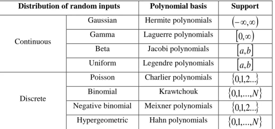
will be omitted for the sake of brevity.

Wiener [1938] first introduced the PCE by adopting Hermite Polynomials as a basis for the approximation of Gaussian processes. Different types of orthogonal polynomials are required for optimum convergence rate in the case of non-Gaussian processes (Table 2.1), as the probability distribution of input parameters influences the choice of the polynomial basis in (2.1). In this regard, Xiu and Karniadakis [2002] introduced the Askey family of hypergeometric polynomials (generalized PCE), to extend the approach to other possible distributions.

Once the appropriate kind of polynomials is identified, the set of independent random variables ζ automatically stems from orthogonality condition, as the multivariate polynomial basis has to be orthonormal with respect to the joint PDF of ζ . The variables collected in ζ are then related to the input parameters in p via a simple isoprobabilistic transform [Sudret, 2008].

Distribution of random inputs Polynomial basis Support

Continuous

Gaussian Hermite polynomials







_,





Gamma Laguerre polynomials



₀

_,





Beta Jacobi polynomials

 

_a,

_b

Uniform Legendre polynomials

 

_a,

_b

Discrete

Poisson Charlier polynomials



₀

_,

₁

_,

₂

_...



Binomial Krawtchouk

polynomials



0

,

1

,...,

N



Negative binomial Meixner polynomials



₀

_,

₁

_,

₂

_...



Hypergeometric Hahn polynomials



₀

_,

₁

_,...,

_N



Table 2.1. Distributions of random input and respective polynomial basis in the

Wiener-Askey scheme.

2.1.2 Computation of the expansion coefficients

The traditional approach for the computation of the expansion coefficients in stochastic finite element analysis consists in the minimization, in the Galerkin sense, of the residual present in the balance equation [Sudret, 2008; Ghanem and Spanos, 1991]. This solving method is identified as intrusive, requiring onerous and specific implementation in the finite element code [Sudret, 2008; Webster et al., 1996].

A non-intrusive regression-based approach, comparable with the response surface method widely used in science and engineering, can be employed to calculate the coefficients aj appearing in (2.1) upon

minimization of the variance of a suitable residual,



, typically defined as the difference between the surrogate model response, y~ , and the solution given by the original model, y , with respect to the vector of the unknown coefficients

a

[Sudret, 2008]:

 







 

 

 



          _  p ζp a a ~ , , 2 2 f f E ArgMin E ArgMin  , (2.2)

with E[·] denoting expected value.

The optimum set of regression points in the (random) parameter space is determined on the basis of the same arguments adopted for integral estimation through Gaussian quadrature; the method employs the roots of the polynomial of one order higher than q, to assure proper sampling of the region associated with largest probability in the distributions of the input parameters (Figure 2.1). The latter approach is denominated the probabilistic collocation method [Huang et al., 2007; Webster et al., 1996].

The vector

a

that optimizes the regression expressed in (2.2) can be determined in form of matrix calculation as



Ψ Ψ



1Ψ y' a T  T , (2.3) where:

 

i j ij   Ψ ,

i



1

,...

N

;

j



0

,...

P



1

. (2.4) Here N is the number of regression points, 'y is the vector denoting

the model response at these points, while the product

Ψ

T

Ψ

defines the so-called information matrix. Solving (2.3) requires a minimum of N P regression points. One typically selects N P to avoid singularity in the information matrix. Figure 2.2 depicts P , that is proportional to the dimension of the problem, against the number of random input parameters, M, for different degrees of the expansion, q. It is possible to observe that even in case of complex models with several parameters, the number of model runs required to compute the PCE surrogate model remains definitely lower with respect to the number of simulations typically

required by Monte Carlo (MC) analysis.

Figure 2.1. Example of sampling in the probability distributions of an input

parameter to constitute the set of regression points.

Figure 2.2. Number of unknown expansion coefficients, P, against M for different

values of q. Input p1 Input p1 PDF of p1 Model; PCE

2.1.3 The Nataf transform

Correlation amongst random parameters can be included in the methodology by applying the Nataf transform [Nataf, 1962].

Let

p





p

₁

,

p

₂

,...,

p

_M



be the vector of correlated random input parameters. When the marginal CDFs, F

 

p_i i M

i , 1,...,

p  , and the

correlation matrix, ρ

 



ij _MM, are known, an isoprobabilistic transform

can be applied to transform p in a vector

z





z

1

,

z

2

,...,

z

M



of standardized

normal random variables:

 



i



i Fpi p

1

z  , i1,...,M, (2.5)

where 1

 

is the inverse standard normal CDF.

The joint probability density function related to the variables collected in

z

is given by:





 

 

       z ρ z ρ ρ z T ₀1 0 0 2 1 exp det 2 1 , M M





, (2.6) where

 

M M ij _  ₀ 0



ρ represents the respective correlation matrix.

According to the Nataf transform theory, the approximate joint PDF

 

p f may be expressed as

 

   

_{   }

_{ }

 



0



2 1 p 2 p 1 p , ... ... 2 1 ρ z p p M M M z z z p f p f p f f M









       . (2.7)

To determine the correlation matrix

 

M M ij _  ₀ 0



ρ in the previous equation, any two random variables



p ,i pj



are considered and the linear

correlation between them results:

 





 

 

_

_

  _                              j i ij j i j j i i ij z z dzdz z F z F j j i i 0 2 p p 1 p p 1 , ,















(2.8) where i p  , j p  , i p  , j p

 are the means and standard deviations of p_i and

j

p respectively.

Once ρ₀ is obtained, it can be decomposed following Cholesky as

T

0 0

0 Γ Γ

ρ   , (2.9)

where Γ₀ is the lower triangular matrix.

Finally the independent and dependent standard normal random vectors,

ζ

and

z

respectively, are related as follows

ζ Γ

z ₀ . (2.10) With the adoption of the Nataf transform the problem of correlation among input parameters is reduced to the set of assumptions required for the application of the PCE [see e.g. Li et al., 2011].

2.1.3 The Karhunen-Loeve Expansion (KLE)

The representation of random fields can be included in this framework based on the PCE theory through the adoption of the Karhunen-Loeve Expansion (KLE) [Ghanem and Spanos, 1991]. The latter characterizes stationary and non-stationary random process in terms of uncorrelated random variables



_k

 



:

 



 



   

 M k k k k x f x x 1 ,      , (2.11)

 

x



being the mean of the process, _k and fk

 

x the eigenvalues and

eigenfunctions of the covariance function

C



x

₁

, x

₂



respectively; M is the number of terms of the expansion.

The deterministic eigenfunctions and the eigenvalues derive from the solution of the homogeneous Fredholm integral equation of the second kind:



x1,x2

  

f x1dx1 f

 

x2 C _{k k k} D



  . (2.12)

For most of the covariance functions, numerical method are required to solve equation (2.12). In this context, the adoption of a traditional Galerkin approach results in dense matrices onerous to be computed and inverted. A more efficient method is adopted in this work, based on a Wavelet-Galerkin scheme proposed in Phoon et al. [2002]. According to this approach from the Haar mother wavelet function,



 

x

, (Figure 2.3) a complete set of orthogonal functions is defined over the domain [0,1] in two steps:

 

x a_j



jx k



k j,  



2 



, (2.13)

 

1,

 

_,

 

, 2 0 x x x i k j k j i    







. (2.14)

Here,

a

_j represents the amplitude of the function (set to 1),

1 ,..., 1 , 0   m

j the dilatation constant and k0,1,...,2j 1 the translational constant respectively;

m

is the maximum wavelet level.

The orthogonality condition can be written as

   

j j ij i x  x dx h        1 0 , (2.15)

where h_i is a constant and



ij represents the Kronecker-delta function.

Figure 2.3. Number of unknown expansion coefficients, P, against M for different

values of q.

In this framework the eigenfunction f_k

 

x can be properly approximated as a truncated series of Haar wavelets:

 

  

 



 

  1 0 ) ( ) ( N i k T i k i k x d x x D f  , (2.16)

where d_i(k) are the wavelet coefficients and N2m [Phoon et al., 2002]. The expression of the covariance function can be obtained through the application of the 2D wavelet transform as follows:



x1,x2



 

x1 A

 

x2 C T   , (2.17)



    

       1 0 1 0 2 1 1 2 2 1, 1 dx dx x x x x C h h A _{i j} j i ji





. (2.18)

The original problem expressed by equation (2.12) is reduced to the following eigenvalue problem:

 

( ) T

 

(k) k k T D x D H A x       



, (2.19) where H is a diagonal matrix constituted by the elements h_i defined in (2.15) [Phoon et al., 2002].

2.2 GLOBAL SENSITIVITY ANALYSIS (GSA)

2.2.1 The ANOVA decomposition and Sobol indices

Consider the model function

y



f

(p

)

, representing the relationship between the random output y and the vector p of M independent random model parameters. Suppose that the latter are defined in the M-dimensional unit hypercube,

I

M

.

If

f

(p

)

is integrable, the following representation holds:

 





M



M



M j i ij i j M i i i p p p f p p f p f f f( ) , ... _{1,2,... 1}, ₂,..., 1 1 0          p (2.20) where M I f d

f₀ (p) p is the mean of the model output and, e.g.,

   1 ( ) _{~ 0} ) ( M I i i i p f d f

f p p , is the function obtained by integrating over all

parameters except pi.

Assuming the validity of the following condition:



,...



0 1 1 1,...     s s s s I i i k k i i i i p p dp f , 1i₁...i_s M ,s1,...M (2.21) where indices i ,...,1 i_s, define the set



p ,...,i1 pis



of random model

condition (2.21) renders representation (2.20), which is typically termed ANOVA decomposition [Archer et al. 1997], unique.

The total variance, V, of the model due to the uncertainty of the M parameters is:

 

        i i M i i I s s M f d f V V ... 1 ,... 2 0 2 1 1 p p , (2.22) where _





  s s s s s I i i k k i i i i i i f p p dp V 1 1 1 1 ,..., 2 ,...

,... is the partial variance, expressing the contribution due to the interaction of parameters



p ,...,i1 pi_s



. The

generic s-order Sobol index

s i i S _,... 1 is defined as [Sobol, 1993]: V V S s s i i i i₁,...  ₁,... (2.23)

The sum of these indices over all possible combinations of parameters is unity. The first-order or principal sensitivity index, S_i, describes the significance of the parameter p_i considered individually, in terms of the fraction of total output variance which is attributed to the variability of p_i

by itself. Higher-order indices Si1,...i_s account for the variance attributable

to the simultaneous variability of a group of parameters. The overall contribution of the variability of a given parameter p_i to the output variance is described by the total sensitivity index ST_i:

  i s i i i T S S  1,... ,



i 





i1,...is



:k,1ks,ik i



. (2.24) The evaluation of the indices (2.23) requires multiple integrations of the model

f





and its square, for various combinations of the parameters. This is traditionally achieved by MC simulation [Sobol, 2001] and the

associated computational cost can soon become prohibitive when the model is complex and/or the number of parameters is large [Sudret, 2008].

2.2.2 PCE and GSA

The entire variability of the original model is conserved in the set of expansion coefficients [Ghanem and Spanos, 1991], rendering PCE a powerful tool for GSA as the Sobol indices can be calculated analytically from these coefficients without additional computational cost [Sudret, 2008]. Manipulating

y~

by appropriate grouping of terms allows isolating the contributions of the different (random) parameters to the system response as:

 

 







M



i i M M i i i M i M s s i i s i a a a a y                  ,..., ... ,..., ~ 1 ... 1 1 0 ,... 2 , 1 1 ... 1 1                      ζ (2.25)

 denoting a general term depending only on the variables specified by the subscript.

The mean of the model response coincides with the coefficient of the zero-order term, a₀, in (2.25), while the total variance of the response and the generic Sobol index, calculated through the PCE, respectively result:

 

_{ }

_{ }



_

_{ }



             1 1 2 2 1 0 ~ P j j j P j j j y E a a Var V ζ ζ , (2.26)  

 

 y y i i V E a S S i is s ~ 2 2 ~ ,... ... 1 1         . (2.27)

Calculation of E

 

_2 can be performed following, e.g., Abramowitz and Stegun [1970].

2.3 THE MATLAB TOOLBOX

This chapter is devoted to the presentation of the developed MATLAB computational framework based on the PCE theory. The numerical tool is designed to be applicable to different environmental and civil engineering scenarios when parameters and boundary conditions are uncertain. In these cases, direct or inverse problems involving, e.g., risk analysis and optimizations under uncertainty need to be solved.

The first version of the code has been thought to be adaptable to different contexts and to be modifiable in straightforward manner. Figure 2.4 depicts the structure of the main program of the toolbox. Following the script, in the first function, Setting ( ), the user is required to set the number of uncertain parameters, M, and the maximum degree of the PCE approximation, q. The latter is typically selected to be equal to 2. If necessary, it is then subsequently increased to improve the accuracy of the approximation. The number of terms of the expansion, P, is then defined. The subsequent step is the definition of the set of regression points (see Section 2.1.2). From the knowledge of the distribution type associated with the uncertain input parameters, the user can choose the polynomial basis that optimizes the convergence rate (see Table 2.1). Figure 2.4 considers a case in which model parameters are uniform distributed and the Legendre Chaos is selected. The Legendre Chaos and the Hermite Chaos are implemented in this first version of the code as they are the most commonly used. In view of this, the function LegendreRegP ( ) returns automatically the set of regression points to optimize the computation of the expansion coefficients. Each regression point corresponds to a combination of values for the vector

ζ

(see Section 2.1.1).

% SFERA v1.0 - MAIN PROGRAM % Version: 25/9/2012 clc clear variables % PROBLEM SETTING Setting();

% REGRESSION POINTS DEFINITION

LegendreRegP(); % PCE GENERATION LegendrePCE(); % REGRESSION-BASED APPROACH TransfRegP(); PCECoef();

% GSA through PCE

LegendreGSA();

Figure 2.4. Basic main program of the MATLAB toolbox

The function LegendrePCE ( ) builds the multivariate polynomial expansion which is then computed at the standardized regression points previously identified. At this stage the coefficients, ai, are still unknown. Note that, up to this point, the only information which is requested from the user are the values of q and M and the identification of the suitable basis of polynomials.

In the subsequent steps the PCE-based surrogate model is defined according to the specific of the particular target scenario, i.e. on the basis of (i) the original analytical or numerical model, and (ii) the uncertainty associated with model parameters. The function TransfRegP ( ) returns the combinations of model parameters collected in p and corresponding to the

standardized regression points

ζ

which were previously computed. As described in Section 2.1.1, p and

ζ

are related via a simple isoprobabilistic transform. This transform is performed by calling the function LegendreIsopTr ( ) as depicted in Figure 2.5 where N is the number of regression points that are collected in the rows of the matrix CSI. The user is required to modify this function by introducing the distributions of the model input parameters for the selected case study.

function TransfRegP() … for i=1:N X(i,:)=LegendreIsopTr(CSI(i,:)); end … end function [X]=LegendreIsopTr(CSI1) PCSI=unifcdf(CSI1,-1,1); %Function test 1 %x1: uniformly distributed in [-0.5;0.5] ax1 = -0.5; bx1 = 0.5; X(1) = unifinv(PCSI(1),ax1,bx1); %x2: uniformly distributed in [-0.5;0.5] ax2 = -0.5; bx2 = 0.5; X(2) = unifinv(PCSI(2),ax2,bx2); end

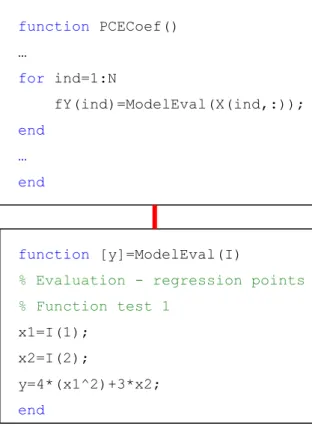
Continuing with the Main program, the function PCECoef ( ), depicted in Figure 2.6, evaluates the original model at the combinations of model parameters corresponding to the standardized regression points and computes the expansion coefficients in vector a trough the regression-based approach described in Section 2.1.2. The function ModelEval ( ) is called in the script. This function is the only part that the user is required to change with the original model considered.

Finally, once the PCE surrogate model is built, the function LegendreGSA ( ) returns analytically the Sobol indices for the GSA, according to what is described in Section 2.2.2.

function PCECoef() … for ind=1:N fY(ind)=ModelEval(X(ind,:)); end … end function [y]=ModelEval(I)

% Evaluation - regression points % Function test 1

x1=I(1); x2=I(2);

y=4*(x1^2)+3*x2;

end

Figure 2.6. Regression-based method for the definition of the PCE

2.4 TEST CASES AND VALIDATION

In this section some application examples of the numerical code developed for PCE-based analysis are provided. A first simple mathematical function is adopted to clarify the key steps run by the code; then a case study in the context of groundwater flow is considered and a comparison against a traditional MC approach is presented. Finally, some examples related to the implementation of the Karhunen-Loeve expansion is provided.

2.4.1 PCE of a polynomial function

We start the illustration of our suite of examples by considering a simple polynomial format which enables one to illustrate the key steps embedded in the application of the numerical code based on the model reduction strategy presented in the first two sections of this chapter.

Consider the model function 2 2 1 2 1, ) 4 3 (p p p p f y   ,

(

p

₁

,

p

₂

)



p

being the vector of uncertain input parameters. Suppose that both

p

₁ and

2

p

are uniformly distributed in the range





0

.

5

;

0

.

5



. The (statistical) moments of y and the Sobol indices can be analytically determined upon calculation of integrals. These theoretical results are compared in the following with those returned by the numerical code. The latter proceeds according to these steps:

 Step 1. Problem setting.

In this test case the number of uncertain parameters is M = 2. The maximum degree selected for the expansion is conveniently set as q = 2. The associated PCE is then formed by P6 terms. The adopted

distributions for the parameters suggests to resort to the Legendre Chaos polynomial basis [Xiu and Karniadakis, 2002]. Therefore, the PCE is expressed in terms of the two random variables,



₁ and



₂, which are uniformly distributed within

 



1

;

1

. Note that



₁ and



₂ represent standardized parameters which are related to

p

₁ and

p

₂ through an isoprobabilistic transform.

 Step 2. Identification of the optimum set of regression points.

The set of regression points is made by pairs





₁

,



₂



which are identified in the parameter space. Values for



₁ and



₂ are chosen amongst the roots of the Legendre polynomial of degree 3 (i.e.,

q



1

) upon imposing the criterion of being closest to the origin and symmetric with respect to it [Webster et al., 1996; Sudret, 2008]. Table 2.2 collects the set of regression points returned by the numerical code for this test case.

1



0 -0.775 0 0.775 0 -0.775 0.775 -0.775 0.775

2



0 0 -0.775 0 0.775 -0.775 -0.775 0.775 0.775

Table 2.2. Regression points for the selected polynomial function test case.

 Step 3. Definition of the Polynomial Chaos Expansion (PCE).

The numerical code calculates the univariate Legendre polynomials of degree included in

 

0

,

q

for each standardized parameter. The summands of the multivariate polynomial of order q are then obtained through all the possible multiplicative combinations (of degree not exceeding q ) between

two univariate polynomials in



₁ and



₂, respectively. The Legendre Chaos expansion of the original model for this test case is:

2 2 5 2 1 4 2 3 2 2 1 1 0 2 1 2 3 2 3 0 ) , ( ~ ~ 1                     f a a a a a a y . (2.28)

 Step 4. Computation of the expansion coefficients.

The expansion coefficients in (2.28) are computed according to the regression based strategy discussed in Section 2.1.2. In this application the number of regression points, N , required to solve the problem is

. 6  P

N The coefficient values returned by the code are:

0 ; 3 2 ; 2 3 ; 3 1 5 4 1 3 2 0  a  a  a a a  a . (2.29)

The second order PCE of the original model is finally obtained by substituting (2.29) in (2.28), i.e.: 2 2 2 1 ₂ 1 3 ) , ( ~ ~_{y f      . (2.30)}

 Step 5. Uncertainty Quantification (UQ) and Global Sensitivity Analysis (GSA).

The mean and variance of

y~

are

3 1 ~ 0 a y and V ~y 0.838, respectively. The calculated partial variances and Sobol indices are presented in Table 2.3. Note that these coincide with the analytical values which can be obtained through integral computation for this simple test case.

 y V1~  y V2~  y S1~  y S2~  y S_1,~₂ ST1 y~  y ST2~ 8 0 . 0 0.75 0.106 0.894 0.000 0.106 0.894

Table 2.3. Variances and sensitivity indices for the polynomial function test case.

2.4.2 PCE for pumping tests in non-uniform aquifers

Let consider a fully penetrating well, deriving a constant flow,

Q

, from a non-uniform confined aquifer. In particular the configuration discussed in Butler [1988] is studied here. In the latter, depicted in Figure 2.7, the well is inserted at the center of a disk of radius R , embedded in an infinite matrix. The disk and the matrix are considered both uniform with respect to the flow properties.

Figure 2.7. Domain schematic.

t s T S r s r r s _i i i i i           1 2 2 . (2.31)

where

s

represents the drawdown in material i ,

r

is the radial direction,

i

S and T_iare the storage coefficient and the transmissivity of material i ( 1



i denotes the disk while i2 denotes the matrix).

To solve the problem the following initial and boundary conditions are set:

Q

r

s

T

r

_w rw









 1 1 0

2

lim



. (2.32)

 

,

0

2



t



s

. (2.33)

   

,

0

₂

,

0

0

,

,

1

r



s

r



r



r





s

_w . (2.34)

where r_w is the radius of the well. Finally conditions of continuity at the disk-matrix interface are included:

   

R

t

s

R

t

s

₁

,



₂

,

_{, (2.35)}

 

 

. , , ₂ 2 1 1 r t R s T r t R s T      (2.36)

An analytical solution of (2.31)-(2.36) is available in the Laplace space:

 

   

     

       

, 2 2 0 1 1 0 1 2 0 1 0 1 2 0 1 1 0 1 1                             AR K NR I AR K NR I N A T T p Nr I AR K NR K N A T T AR K NR K T Q p Nr K T Q s





(2.37)

   

   





 

       

, 2 0 1 1 0 1 2 0 0 1 1 0 1 2                AR K NR I AR K NR I N A T T p Ar K NR I NR K NR I NR K T Q s



(2.38)

where

s

₁,

s

₂ represent the transformed drawdown in the Laplace space, p is the Laplace-transform variable,

I

j is the modified Bessel function of the

first kind and order j, Kj is the modified Bessel function of the second

kind and order j, and N S₁p T₁ and A S₂p T₂ . Equations (2.37)-(2.38) require a numerical inversion with e.g. the algorithm of Stehfest [1970].

Starting from this formulation [Butler, 1988] a specific case study is defined in which the uncertain model parameters are the transmissivities of the disk and the matrix and the storage coefficients, considered equal for the two materials. Each of these three variables is associated with a log-normal distribution and coefficient of variation equal to 0.5. The means of the distributions are



_S



5



10

6, _T 8 103m2/s

1   



, _T 5 10 3m2/s 2   



(values typical of sand). The model responses of interest are the drawdowns in the two materials.

The PCE of second, third and fourth order are adopted as surrogate models on which GSA is performed.

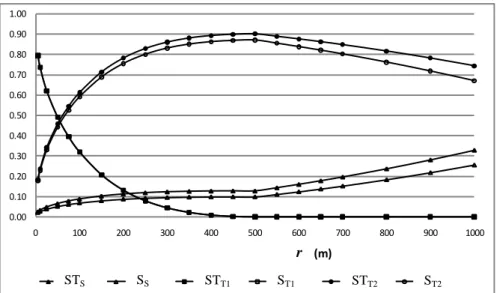
Figure 2.8 depicts the total sensitivity indices related to the three uncertain parameters versus the radial distance from the well. It’s observable that the influence of S increases far from the well while the reverse is true for

T

₁. The importance of the uncertainty in

T

₂ has a maximum value at the interface between the two materials. The

interactions among the parameters is negligible as total and principal sensitivity indices are significantly similar.

Figure 2.8. Total and principal sensitivity indices computed with the PCE of order

2 (R = 500 m ; t = 5000 s ; Q = 0.01 m3/s).

Figure 2.9. Comparison between the total sensitivity indices computed with the

PCE of order 2 (Pol2) and through a traditional Monte Carlo framework (number of simulations = 1000, 5000).

As the sensitivity indices are almost constants with respect to the degree of the expansion (not shown), the results depicted are referred to the second order. 0.00 0.10 0.20 0.30 0.40 0.50 0.60 0.70 0.80 0.90 1.00 0 100 200 300 400 500 600 700 800 900 1000 distanza radiale dal pozzo (m)

IST di S ISP di S IST di T1 ISP di T1 IST di T2 ISP di T2

0.0 0.2 0.4

0 100 200 300 400 500 600 700 800 900 1000

distanza radiale dal pozzo

IST di S Pol2 IST di S MC1000 IST di S MC5000

0.0 0.2 0.4 0.6 0.8 1.0 0 100 200 300 400 500 600 700 800 900 1000

distanza radiale dal pozzo

IST di Pol2T1 IST di MC1000T1 IST di MC5000T1

0.0 0.2 0.4 0.6 0.8 1.0 0 100 200 300 400 500 600 700 800 900 1000

distanza radiale dal pozzo

IST di Pol2T2 IST di MC1000T2 IST di MC5000T2

r

STS SS STT1 ST1 STT2 ST2

STS STT1 STT2

r r r

In Figure 2.9 a comparison between the sensitivity measure computed through PCE and a traditional MC framework is shown. The results of PCE appear substantially confirmed; furthermore, the latter tend to the MC-based values as the number of MC simulations increases. The advantage in terms of accuracy is added to the computational saving, equal to three orders of magnitude for the examined case.

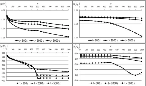
Figure 2.10. Variance maps for different times computed through the second-order

PCE.

Figure 2.10 reports the maps of variances (total and partials) inside the domain for different times. For early times the drawdown in the disk is influenced only by the local properties of the system while the transmissivity of the matrix does not produce effects. This is physically consistent because the drawdown is initially confined in the material around the well. On the contrary, when tending to the stationary condition the process is dominated by the properties of the matrix even if around the well the transmissivity of the disk conserves a relevant effect. For what

-3.00 -2.00 -1.00 0.00

0 100 200 300 400 500 600 700 800 900 1000

distanza radiale dal pozzo

t = 300 s t = 2000 s t = 5000 s

-3.00 -2.50 -2.00

0 100 200 300 400 500 600 700 800 900 1000

distanza radiale dal pozzo

t= 300 s t = 2000 s t = 5000 s -7.00 -6.00 -5.00 -4.00 -3.00 -2.00 -1.00 0.00 0 100 200 300 400 500 600 700 800 900 1000

distanza radiale dal pozzo

t = 300 s t = 2000 s t = 5000 s -6.00 -5.00 -4.00 -3.00 -2.00 -1.00 0 100 200 300 400 500 600 700 800 900 1000

distanza radiale dal pozzo

t= 300 s t = 2000 s t = 5000 s  V ln ln VS

 

1 lnVT ln

 

VT2 r r r r

concerns the drawdown in the matrix, the process is influenced only by the local properties, especially for late times.

2.4.3 KLE of some known covariance functions

In order to test the implementation of the Karhunen-Loeve Expansion according with the numerical method discussed in section 2.1.3, some well known covariance functions are here considered and the results obtained in Phoon et al. [2002] are adopted as a comparison.

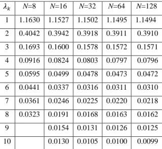
1) Test covariance function 1: first-order Markov process defined in [-1;1]; exponential covariance function _.

The eigenvalues obtained with the implemented code are reported in Table 2.4. N=8 N=16 N=32 N=64 N=128 1 1.1630 1.1527 1.1502 1.1495 1.1494 2 0.4042 0.3942 0.3918 0.3911 0.3910 3 0.1693 0.1600 0.1578 0.1572 0.1571 4 0.0916 0.0824 0.0803 0.0797 0.0796 5 0.0595 0.0499 0.0478 0.0473 0.0472 6 0.0441 0.0337 0.0316 0.0311 0.0310 7 0.0361 0.0246 0.0225 0.0220 0.0218 8 0.0323 0.0191 0.0168 0.0163 0.0162 9 0.0154 0.0131 0.0126 0.0125 10 0.0130 0.0105 0.0100 0.0099

Table 2.4. Eigenvalues of the first-order Markov process for different maximum

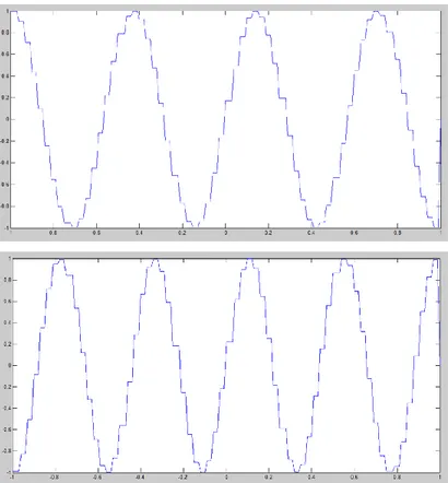
For this test case, Figure 2.11 also depicts the 8th and 10th order eigenfunctions.

Figure 2.11. 8th and 10th order eigenfunctions for exponential covariance

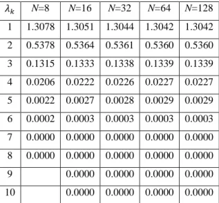
2) Test covariance function 2: Random process defined in [-1;1]; squared exponential covariance function _.

The eigenvalues obtained with the implemented code are reported in Table 2.5.

3) Test covariance function 3: Wiener–Levy process in [0,1]; covariance function .

The eigenvalues obtained with the implemented code are reported in Table 2.6. N=8 N=16 N=32 N=64 N=128 1 1.3078 1.3051 1.3044 1.3042 1.3042 2 0.5378 0.5364 0.5361 0.5360 0.5360 3 0.1315 0.1333 0.1338 0.1339 0.1339 4 0.0206 0.0222 0.0226 0.0227 0.0227 5 0.0022 0.0027 0.0028 0.0029 0.0029 6 0.0002 0.0003 0.0003 0.0003 0.0003 7 0.0000 0.0000 0.0000 0.0000 0.0000 8 0.0000 0.0000 0.0000 0.0000 0.0000 9 0.0000 0.0000 0.0000 0.0000 10 0.0000 0.0000 0.0000 0.0000

Table 2.5. Eigenvalues of the squared exponential covariance for different

maximum Wavelet levels of the Wavelet-Galerkin approach.

N=8 N=16 N=32 N=64 N=128 1 0.4066 0.4056 0.4054 0.4053 0.4053 2 0.0464 0.0454 0.0451 0.0451 0.0450 3 0.0176 0.0165 0.0163 0.0162 0.0162 4 0.0097 0.0086 0.0084 0.0083 0.0083 5 0.0065 0.0053 0.0051 0.0050 0.0050 6 0.0050 0.0037 0.0034 0.0034 0.0034 7 0.0043 0.0028 0.0025 0.0024 0.0024 8 0.0039 0.0022 0.0019 0.0018 0.0018 9 0.0018 0.0015 0.0014 0.0014 10 0.0015 0.0012 0.0011 0.0011

Table 2.6. Eigenvalues of the Wiener-Levy process for different maximum