1 TITLE
1D ELASTIC FULL-WAVEFORM INVERSION AND UNCERTAINTY ESTIMATION BY 3
MEANS OF A HYBRID GENETIC ALGORITHM-GIBBS SAMPLER APPROACH
Aleardi Mattia, Mazzotti Alfredo 6
University of Pisa, Earth Sciences Department Via S. Maria 53, 56126, Pisa (Italy)
2
ABSTRACT
Stochastic optimization methods such as Genetic Algorithms (GA’s) search for the global 12
minimum of the misfit function within a given parameter range and do not require any calculation of the gradients of the misfit surfaces. More importantly, these methods collect a series of models and associated likelihoods that can be used to estimate the posterior probability distribution (PPD). 15
However, because GA’s are not a Markov Chain Monte Carlo method (MCMC), the direct use of the GA-sampled models and their associated likelihoods produce a biased estimation of the PPD. In contrast, MCMC methods, such as the Metropolis-Hastings and Gibbs sampler, provide accurate 18
PPDs but at considerable computational cost. In this work, we use a hybrid method that combines the speed of GA to find an optimal solution and the accuracy of a Gibbs Sampler (GS) to obtain a reliable estimation of the posterior probability distributions. First, we test this method on an 21
analytical function and show that the GA method cannot recover the true probability distributions and that it tends to underestimate the true uncertainties. Conversely, combining the GA optimization with a GS step enables us to recover the true PPD. Then, we demonstrate the 24
applicability of this hybrid method by performing 1D elastic Full-Waveform Inversions (FWI) on synthetic and field data. We also discuss how an appropriate GA implementation is essential to attenuate the “genetic drift” effect and to maximize the exploration of the model space. In fact, a 27
wide and efficient exploration of the model space is important not only to avoid entrapment in local minima during the GA optimization but also to ensure a reliable estimation of the posterior probability distribution in the subsequent GS step.
3
KEYWORDS
Full-waveform inversion, Elastic, Stochastic. 33
4 Introduction
36
Full-waveform inversion (FWI) is a data-fitting procedure that is based on full-wavefield modelling to extract quantitative information from seismograms (Tarantola, 1986). The aim is to exploit the full information content of the data to derive high-resolution quantitative models of the 39
subsurface. Most recent developments have focused on building P-wave velocity models to be used as improved background velocity fields for wave equation depth migration (Vireux and Operto, 2009; Sirgue et al. 2010; Prieux et al. 2011; Morgan et al. 2013). In this context, the FWI is usually 42
solved in the acoustic approximation and by applying gradient-based methods (such as the Gauss-Newton or conjugate gradient). A limitation of the gradient-based methods is their local nature and the consequent requirement of a good starting model to avoid convergence toward local minima. A 45
way to overcome this problem is to use stochastic optimization methods, which are less affected by the presence of local minima in the misfit function but require huge computational efforts.
Stochastic FWI was first performed in the 1990s to invert single-shot gathers, assuming an 48
acoustic approximation and 1D geological models. In this context, the limited number of model parameters made it possible to apply global optimization techniques, such as simulated annealing and genetic algorithms (Sen and Stoffa, 1991; 1992). For many practical applications, the stochastic 51
approach to elastic FWI is usually limited to horizontally stratified media using reflectivity method (Mallick, 1999; Mallick and Dutta 2002; Mallick et al. 2010; Fliedner et al. 2012; Li and Mallick, 2015). It is known that the computational cost of stochastic methods grows exponentially with the 54
number of unknowns. Such scaling problem is sometimes referred to as the “curse of dimensionality” (Bellman, 1957) and it makes the stochastic, elastic, FWI unfeasible for 2D or 3D applications in which thousands or even millions of unknowns are considered. However, thanks to 57
the recent growth of high performance computing, the stochastic approach to FWI begins to be used to derive accurate, low-resolution, 2D or 3D compressional velocity fields that are well-suited to play the role of starting models for gradient-based, acoustic, FWI (Sajeva et al. 2014a; Gao et al., 60
5
2014; Tognarelli et al. 2015; Datta, 2015). In these applications a method to reduce the number of unknown parameters and a highly efficient parallel implementation are crucial to make the computational cost of the stochastic inversion affordable (Diouane et al. 2014; Sajeva et al. 2014a). 63
The extension of this two-step approach, based on a global (low-resolution) inversion followed by a local (high-resolution) inversion, to the elastic case is not the topic of the present work but deserves deeper investigation.
66
Many global derivative-free methods perform a wide exploration of the multidimensional parameter space and collect many different models. However, it is the single model producing the best fit with the observed data that focuses our attention, while the other models are often neglected. 69
In this way, we fail to quantify the uncertainty that characterizes the final result. Instead, inverse problems can be solved in a probabilistic framework (Dujindam, 1988; Tarantola, 2005) in which the final solution is represented by posterior probability distributions (PPDs) in model space (see 72
Appendix A for a brief review of the Bayesian formulation of inverse problems).
Among the many global search methods that have been proposed to solve 1D full-waveform inversion, we choose to apply genetic algorithms (GA’s). Likewise other global search algorithms, 75
GA’s are not a Markov Chain Monte Carlo (MCMC) method (Rubinstein and Kroese, 2011), and a biased PPD is estimated if directly computed from the set of GA-sampled models and their associated likelihoods. To derive an unbiased PPD estimation, a simple grid-search method or a 78
more sophisticated MCMC algorithm must be applied (Sen and Stoffa, 1996). However, the direct application of these methods is not feasible for high dimensional model spaces due to their high computational costs. Therefore, several methods that follow the solution of 1D FWI by means of 81
GA optimizations (Sen and Stoffa, 1996; Mallick, 1999; Hong and Sen, 2009) or via local optimizations (Gouveia, and Scales, 1997, 1998) have been developed to obtain reliable and unbiased estimates of the posterior distributions. Another strategy based on ensemble Kalman filter 84
(Evensen, 2009) has been proposed in the context of 1D elastic FWI to reduce the number of unknowns and to perform a statistical analysis of the final result (Jin et al. 2008).
6
In the present study, we combine an implementation of the GA method with a resampling of the 87
explored model space by means of a MCMC method known as Gibbs Sampler (GS) (Geman and Geman, 1984). This hybrid approach attempts to combine the speed of GA’s and the unbiased nature of GS to obtain reliable estimates of the uncertainties that affect the final result. In particular, 90
the GS exploits all the models and their respective likelihoods that were collected during the GA inversion to compute the posterior probability distributions in model space. Sambridge (1999) proposed the same hybrid strategy in the context of neighbourhood algorithm inversion. However, 93
as discussed in Sajeva et al. (2014b), the neighbourhood algorithm seems to show a slower convergence compared to GA in solving 1D elastic FWI.
To achieve a reliable estimation of the posterior probability distributions, the first step of GA 96
optimization must perform a wide exploration of the model space because an insufficient GA sampling of the model space cannot be compensated for by the subsequent GS step. In this regard, GA optimization suffers from the “genetic drift” effect (Goldberg and Segrest, 1987; Horn, 1993), 99
which limits the exploration of the model space and may guide the algorithm to prematurely converge toward a local minimum. To address this issue, we apply a GA implementation that combines the Niched-GA (N-GA) method with other mechanisms, such as migration, competition 102
between subpopulations, and the stretching of the fitness function to maximize the exploration of the model space and to reduce the genetic drift.
In this work, the GA+GS approach for FWI is applied to derive a complete elastic 105
characterization of the subsurface, assuming wave propagation in 1D elastic models. We start with a brief summary of genetic algorithms that introduces the reader to our particular implementation of GA optimization. Then, we discuss an example on an analytical misfit function to demonstrate the 108
applicability of the hybrid method and the importance of attaining a wide exploration of the model space during GA optimization. The next section illustrates a synthetic FWI example in which the number of layers and their thicknesses are assumed to be known to avoid the overparameterization 111
7
demonstrate the capability of our peculiar GA implementation to attenuate the genetic drift and to maximize the exploration of the model space. To this end, we make use of self-organizing maps (de 114
Matos et al. 2006) to visualize and compare the different model space explorations that are produced by standard GA and by our GA implementation. The second synthetic example is more complex because the 1D elastic model is derived from actual well log data. As in Mallick and Dutta 117
(2002), we overcome the over-parameterization problem by fixing the layers’ thicknesses to constant values based on the dominant frequency that characterizes the observed seismic data. Finally, we present a field case inversion that is performed on a single shot gather that was extracted 120
from a Well Site Survey (WSS), where no a priori information in the form of borehole logs or geotechnical data is available. In all the FWI examples that we discuss, the reflectivity algorithm (Kennett, 1983) is used for forward modelling.
123
A brief introduction to genetic algorithms
Genetic algorithms are search algorithms based on the mechanics of natural selection and 126
evolution according to the Darwinian principle of “survival of the fittest” (Holland, 1975). The GA optimization process is always driven by three main genetic operators: selection, cross-over and mutation. A population of individuals, which encodes candidate solutions to an optimization 129
problem, evolves toward better solutions by starting from a population of randomly generated individuals. The fitness, namely, the goodness of each candidate solution, is evaluated in each iteration (or “generation”), and then multiple individuals are stochastically selected from the current 132
population based on their fitness (models with higher fitness are more likely to be selected). The selected models are then modified (using crossover and mutation operators) to form a new population, which is used in the next iteration.
135
In the fitness assignment, each individual in the selection pool receives a reproduction probability depending on its own misfit value and the misfit values of all the other individuals. The fitness value for each individual can be determined either directly from its associated misfit or by 138
8
applying a rank-based fitness assignment. Bäck and Hoffmeister (1991) observed that the latter approach is more robust than proportional fitness assignment and thus is the method that is applied in this work. In the successive step, the models are selected for reproduction and several selection 141
methods can be used to this goal. See Goldberg and Deb (1991) or Blickle and Thiele (1995) for an extensive comparison and discussion about selection schemes that can be used in a GA optimization. The next step of cross-over produces new individuals by combining the information 144
(namely, the value of each variable) of two or more parents. Finally, in the mutation step randomly created values are added to the variables with a low probability to prevent premature convergence and to escape from local minima. After the parents have been subjected to these operations, the 147
generated offspring has to be reinserted to replace the parents to form the new population. We use an elitist reinsertion, which preserves the fittest individuals of the previous generation in the new generation, combined with a fitness-based reinsertion in which the lowest-fitness parents are 150
replaced by higher-fitness offspring.
Our GA implementation and the hybrid GA+GS method 153
In this work, we adopt a more sophisticated version of GA that is called a niched GA (N-GA), which is based on the punctuated equilibria evolutionary theory (Gould and Eldredge, 1977). According to this method, the initial random population is divided into multiple subpopulations, 156
which are subjected to separated selection and evolution processes (Goldberg, 1989; Mitchell, 1998). The N-GA method has been demonstrated to avoid the genetic drift effect (Horn, 1993), which is the loss of diversity inside a single population that can lead to a local minimum in the case 159
of multimodal misfit functions.
To further improve the exploration of the model space, we apply different evolution strategies for different subpopulations. Therefore, the entire set of subpopulations evolves according to 162
different selection methods, mutation operators and fitness assignment methods. Tanese (1987) demonstrated that this approach, in which different evolution strategies are simultaneously applied,
9
increases the capability of GA to explore the entire model space. In addition to these strategies, we 165
shrink the mutation range and stretch the fitness function (Sen and Stoffa, 1991, 1992) by increasing the selective pressure in each generation. The mutation range is the range that contains the admissible values that a mutated variable can assume, whereas the selective pressure is the 168
probability of the best individual to be selected compared with the average selection probability of all individuals. In particular, we set a small selective pressure value for the initial generations to ensure maximum genetic variance within each subpopulation. In this way, models with similar 171
fitness values have similar likelihoods of being selected, which results in a more efficient and wide exploration of the model space. Conversely, we set a higher selective pressure at the end of the inversion, when the most promising zones of the misfit function have been reached. In this way, 174
minor differences in the fitness values are exaggerated, which results in a fine tuning of the solution. In the following FWI tests, the selective pressure linearly increases with the number of iterations. We also adopt competition between subpopulations, where the best fitting subpopulations 177
are awarded with some individuals from the less-fitting ones to better explore the most promising portions of the model space (Schlierkamp-Voosen and Mühlenbein, 1996).
The FWI tests that follow are quite similar in terms of the number of unknowns (21 and 60 180
unknowns in the two synthetic inversions and 48 in the field data inversion) and thus we can keep the same GA setting for all the tests. In particular, we use a population of 400 individuals, which evolves into 40 generations and is divided into 10 subpopulations, for more than 13000 forward 183
model evaluations. In all cases, we apply a selection rate of 0.8 (we select 80% of the parents for reproduction) and a mutation rate that is the reciprocal of to the number of unknowns, whereas migration and competition between subpopulations occur every 8 and 5 iterations, respectively. 186
Concerning the mutation rate Schlierkamp-Voosen and Mühlenbein (1993), performing GA optimizations and considering from 2 to 100 unknowns, demonstrated that the best choice for the mutation rate is the reciprocal of the number of unknowns. In this way, on average, just one variable 189
10
between observed and modelled seismic data is considered as the misfit function. In all cases, different evolution strategies for each subpopulation, stretching the fitness function and shrinking 192
the mutation range, are included during the iterations. In particular, among the many rank-proportionate selection methods available, we use the stochastic universal sampling, roulette wheel selection and tournament selection methods and we apply linear and non-linear fitness assignments. 195
More detailed information about these and other GA principles can be found in Goldberg (1989), Mitchell (1998) or Sivanandam and Deepa (2008).
There is no unique rule to set the GA parameters, as the best GA setting strongly depends on the 198
problem under examination and in particular on the number of unknowns and on the complexity of the misfit function. For these reasons the best setting for the GA parameters is usually found by trial and error. Basing on our experience on GA optimization for FWI, the heuristic rules we have 201
followed are briefly summarized below. The number of individuals must be always higher than the number of unknowns: in case the misfit surfaces are complicated, it should be 10 or 20 times the number of unknowns. Instead, in case of simple convex misfit surfaces 2 or 3 times the number of 204
unknowns should suffice. Also the choice for the number of subpopulations strongly depends on the number of local minima that we suppose characterizes the misfit function. In our experiments, we found that 5 to 10 subpopulations are required for performing an efficient exploration of the model 207
space. Concerning the selection rate, we found that a value between 0.8-0.9 is usually a good compromise between preserving genetic variance and ensuring an efficient selection process. Different criteria can be used to stop a GA optimization. For example the inversion can be stopped 210
when no further improvements can be seen in the data misfit evolution. This is the stopping criterion adopted in this work. Another possible stopping criterion is based on the difference between the mean and the minimum data misfit. In fact, as noted by Reeves and Rowe (2002), the 213
approaching of mean misfit toward the minimum misfit indicates a loss of genetic diversity. When the genetic diversity is low, the genetic optimization is less efficient and it may be convenient to stop the inversion.
11
Once the GA inversion has stopped, it is possible to create an approximate PPD for the GA solution (Sen and Stoffa, 1992) that we name the GA PPD, which, as previously said, suffers from several limitations. Therefore, we apply the Gibbs sampler method to efficiently estimate the PPD 219
for each variable. The mathematical formulation of the GS step is detailed in Sambridge (1999) together with recipes for practical applications. Thus, only a brief summary is given in Appendix B. To derive the final PPD, the explored model space is divided into Voronoi cells that are centred on 222
each model found by the GA inversion and the likelihood value of the model is assigned to the whole cell. The model space is then resampled by running a Gibbs sampler, which extracts a sequence of random samples from a specific probability distribution. The GS algorithm is 225
frequently applied when direct sampling is difficult, such as when the analytical formulation of the distribution is not known explicitly and it is only numerically defined. The sequence of random samples is used to approximate the joint or the marginal distributions of the variables. Other authors 228
have demonstrated (see, for example, Gelman et al. 2013) that the sequence of samples drawn by a GS algorithm constitutes a Markov chain. Because the likelihood values that are required by the Gibbs sampler are known from the approximate GA PPD, no additional forward model is needed. 231
This characteristic is particularly important because it determines the low computational cost of the GS step.
In general, multiple GS walks are sequentially performed to increase the reliability of the results, 234
and the results of each step are combined to derive the final probability distributions. However, the samples drawn at the beginning of the chain (during the so called “burn-in period”) may not accurately represent the desired distribution (Sambridge, 1999). Therefore, we do not include these 237
samples in the evaluation of the final PPD. In the following inversion examples, we use 100 different GS walks in which 2000 random samples are drawn from the GA PPD. From these 2000 samples, only the second half is used to compute the final probability distributions. During the 240
computation of final PPDs, we consider uninformative prior distributions that are uniformly distributed over the entire search range for each inverted parameter. In this context, the final
12
probability distributions are mainly determined by the likelihood functions (see Appendix A for 243
further details). To verify if the Gibbs sampler has reached a stable distribution, it is important to check the Potential Scale Reduction (PSR) factor (see Appendix B) which gives an indication on the reliability of estimated PPDs.
246
Testing the GA+GS method on an analytical function
We perform a test that uses an analytical function to demonstrate the potential of this hybrid 249
approach to attain an unbiased estimation of the marginal and joint posterior probability distributions. In this test, the GA+GS method is employed to draw samples from a 2D joint PPD p(x1, x2) with a double peak structure, taken from Hong and Sen (2009). Due to the simplicity of the
252
function, and to evidence the need of an accurate exploration of the model space, we employ a standard single-population GA optimization instead of the more sophisticated implementation that was previously described. This simple 2D example allows us to compare both the true joint PPD 255
and the joint PPD that is estimated by the GA+GS method. As shown in equation 1, the considered PPD is the sum of two bivariate normal distribution probability density functions PDF1(x1, x2) and
PDF2(x1, x2), in which a factor of 0.5 ensures that the resulting posterior distribution is properly
258 normalized:
( , ) ( , )
(1) 5 . 0 ) , (x1 x2 PDF1 x1 x2 PDF2 x1 x2 PDF = +The bivariate normal distribution of equation 1 can be re-written in the following form: 261 ) 2 ( ) 1 ( 2 exp ) 1 ( 2 1 ) , ( 2 22 11 2 2 1 − − − = z x x PDF
where σ represents the covariance matrix:
) 3 ( 22 21 12 11 = 264
13 ) 4 ( ) , ( 22 11 12 2 1 =corr x x = and z is equal to 267 ) 5 ( ) ( ) ( ) )( ( 2 ) ( 22 2 2 2 5 . 0 22 11 2 2 1 1 11 2 1 1 − + − − − − = x x x x z
The analytical distribution PDF1(x1, x2) is characterized by a mean vector equal to μ = (0,0) and a
covariance matrix equal to 270 ) 6 ( 1 0 0 1 =
The matrix in equation 6 indicates that x1 and x2 are uncorrelated to each other and thus the
correlation coefficient is 0. The distribution PDF2(x1, x2) has a mean vector of μ = (4, 0) and a
273
covariance matrix given by
) 7 ( 2 8 . 0 8 . 0 2 =
Therefore, x1 and x2 are correlated to each other in this case, with a correlation coefficient equal
276
to 0.4. By summing PDF1(x1, x2) and PDF2(x1, x2) as described in equation 1, the resulting joint
PDF(x1, x2) is a bimodal surface (Figure 1a) with one peak at (0,0) and the second peak at (4,0).
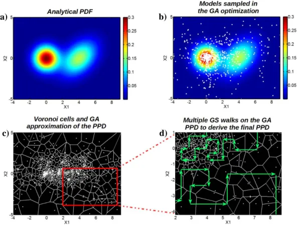
In Figure 1, we give a visual representation of the different steps that characterize the GA+GS 279
approach. Figures 1a and 1b represent the analytical PDF and the ensemble of 1000 models (white dots) that result from the GA optimization on the joint PDF p(x1, x2), respectively. The Voronoi
cells, which divide the entire model space that is explored by the GA optimization, are shown in 282
Figure 1c, while the multiple GS walks that are used to draw random samples from the GA PPD are illustrated in Figure 1d. According to Sambridge (1999), the random GS walks allow the computation of the final GA+GS estimation of the PPD. As expected, the sampling performed by 285
the GS algorithm is denser in the upper left corner of Figure 1d, which is where the GA’s focused the exploration of the model space. However, the GS, differently from the GA sampling, respects
14
the importance sampling principle (Rubinstein and Kroese, 2011) and allows for a highly accurate 288
estimation of the final posterior probabilities.
The marginal PPD is a projection of the joint PPD to a particular parameter axis and can be obtained by integrating out all the other parameters. The true marginal PPDs for x1 and x2 are shown
291
by the green lines in Figures 2a and 2b, respectively. The marginal PPD for x1 is a bimodal
distribution, whereas that for x2 is a univariate normal distribution. We now aim to compare the
marginal and joint PPDs that are estimated after the GA optimization and GA+GS method with the 294
true values. To this end, we compute the marginal GA PPDs on the GA ensemble of 1000 models (orange bars in Figures 2a and 2b) following Sen and Stoffa (1992). We then refine the marginal GA PPDs by running a GS to derive the final GA+GS marginal PPDs (blue curves in Figures 2a 297
and 2b).
Figure 1: Examples of the different steps that characterize the hybrid GA+GS approach. a) The 300
initial analytical PDF used in the optimization. b) The 1000 models (white dots) sampled during the GA optimization. c) The model space portion explored during the GA step is divided into Voronoi
a) b)
d) c)
15
cells (delimited by the white lines), and the likelihood that is associated with each explored model is 303
assigned to the entire cell. This step results in the GA approximation of the PPD. d) Multiple GS walks (examples of GS walks are illustrated by the green paths) are used to draw samples from the GA approximation of the PPD. This step gives the final PPD that was estimated by the GA+GS 306
approach.
309
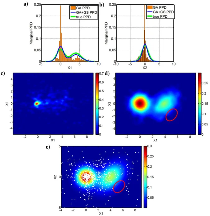
Figure 2: In a) and b), comparisons are shown for the variables x1 and x2 from the true marginal
distributions (green lines), the marginal PPDs that were estimated by the GA method (orange bars)
a) b)
c) d)
16
and the GA+GS marginal PPD estimations (blue lines). c) The GA approximation of the joint 312
distribution. Note the strong underestimation of the uncertainties that resulted from the oversampling of the model space region with the highest probability. d) The final joint PPD estimated by the GA+GS method (compare with the true joint probability distribution shown in e) 315
and the GA joint estimation shown in 1c). Note the different colour-scale in c) and d). e) The true joint posterior distribution (in colour) defined by equation 1 and represented in Figure 1a. The white dots represent the 1000 models sampled in the GA optimization. The red circle in d) and e) 318
marks the area where the differences between the true and estimated GA+GS joint PPDs are more prominent. See the text for additional comments.
321
The GA method tends to oversample the region with high probability and thus underestimates the true uncertainties. In contrast, the hybrid GA+GS method yields marginal PPD estimations that are very similar to the true values. The joint GA PPD (Figure 2c) severely underestimates the 324
variance that is associated with the inverted parameters, whereas it strongly overestimates the probability that is associated with the peak at (0,0). Moreover, the bimodality of the true distribution and the correlation between x1 and x2 in the PDF2(x1, x2) in this approximated PPD are completely
327
lost. Instead, the GA+GS joint PPD that is shown in Figure 2d nicely matches the true joint probability distribution of Figure 2e. Figure 2d also shows that the GA+GS method can predict the correlation between x1 and x2 in PDF2(x1, x2) as evidenced by the slope of the estimated PPD near
330
the secondary peak at (4,0). The main differences between the true and the GA+GS joint PPDs occur in the areas that are highlighted by the red circles in Figures 2d and 2e. In fact, the PPD values in Figure 2e are between 0.05 and 0.1, whereas those in Figure 2d are very close to zero, 333
which indicate an underestimation of the PPD function due to an insufficient sampling by the GA method (the GA’s sampled only two models in this area). Therefore, the importance of an accurate exploration of the model space in the GA optimization, which the standard GA method was unable 336
17
genetic drift effect. However, this analytical example also demonstrates that the hybrid GA+GS algorithm is a reliable method for uncertainty analysis.
339
First synthetic example: exact parameterization
The reference model is a geological sequence that was extracted from the Ocean Drilling 342
Program (ODP) database (http://www-odp.tamu.edu/) and includes a total of eight layers, whose thicknesses, P-wave velocities (Vp), S-wave velocities (Vs) and densities are shown in Figure 3 (black curves).
345
Figure 3: Comparison between the true (black) and predicted (red) elastic properties (a, b and c for Vp, Vs and density, respectively). The grey lines show the parameter ranges used during the 348
inversion.
The reference synthetic seismogram, which was computed by the reflectivity method, consists of 351
30 traces that are spaced by 100 m with a minimum offset of 100 m. The source signature is a 5-Hz Ricker wavelet. To estimate the capability of our algorithm to explore the model space, we set a wide search range for each parameter: +/- 400 m/s for Vp and Vs and +/- 0.4 g/cm3 for density, 354
centered around the true parameter values.
18
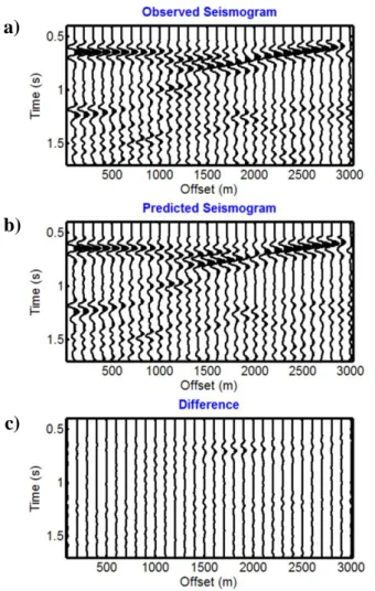
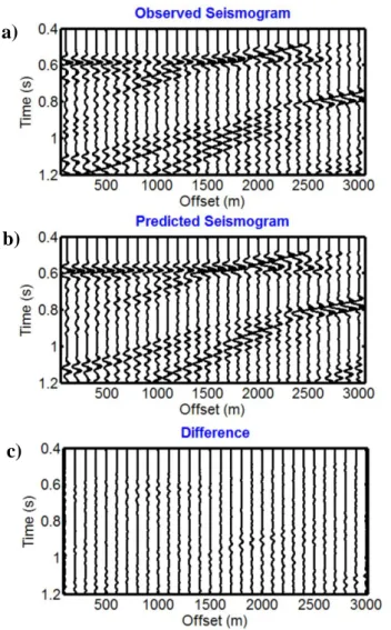
Figure 4: a) Observed seismogram, b) best predicted seismogram and c) their difference. The 357
seismograms are NMO-corrected for the water velocity and are represented with the same amplitude scale.
360
Overparameterization is a well-known issue in inverse problems, which is caused by too many correlated unknowns being introduced into the inversion. For example, overparameterization can be produced if the thicknesses and the number of layers are left unknown or by simultaneously 363
inverting the P-wave velocity and the thickness of each layer. In fact, many combinations of Vp and layer thickness give rise to almost identical reflection kinematics. The overparameterization severely aggravates the ill-posedness of the inverse problem and increases the number of local 366
minima in the misfit function. To avoid overparameterization in this example, we set the layer thicknesses and the water properties to their true values.
b)
c) a)
19
Figures 3a, b and c show a comparison between the best predicted model and the true one. The 369
Vp values are totally recovered, whereas the results are less accurate for Vs and, particularly, for density. Figures 4a, b and c show the observed and best predicted seismograms and their difference, respectively. Note the good results in terms of data misfit. Figures 5a, b and c show the evolution of 372
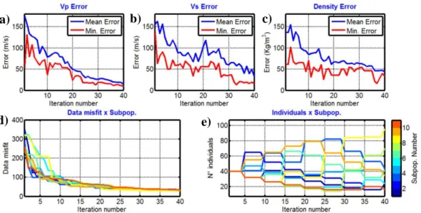
the mean model misfit (blue curve) and the minimum model misfit (red curve) that were computed when considering the entire set of ten subpopulations for the Vp, Vs and density, respectively. The model misfit is computed as follows:
375 ) 8 ( | | 1 1
= − = N i pre i true i m m N Misfit Modelwhere N is the total number of layers (excluding the water column) and mtrue and mpre are the true and current predicted models, respectively. The final model misfit for Vp (Figure 5a) is smaller than 378
the Vs model misfit, and the evolution of the Vs and density model misfits are characterized by more irregular trends that indicate that the seismogram is more sensitive to Vp perturbations than to variations in the other two variables. The differences between the mean and minimum model misfit 381
curves tend to decrease during the inversion as the algorithm converges to a good fitting model. The 10 subpopulations show different data misfit evolutions (Figure 5d) as they explore different parts of the model space. Jumps occur when competition and migration take place. The evolution of 384
the number of individuals for each subpopulation is shown in Figure 5e: all of the subpopulations have the same number of individuals (40 individuals) in the first iteration, and this number changes every 5 iterations when competition occurs. Due to competition, the most successful subpopulations 387
(those that explore the most promising portion of the model space) attract individuals from the less successful ones. At the end of the inversion, the best subpopulation (number 8, yellow curve in Figure 5e) has more than doubled its number of individuals. Conversely, fewer than 20 individuals 390
20
Figure 5: Evolution of the mean and the best model misfit for the Vp, Vs and density parameters 393
as a function of iteration number (a, b and c, respectively). Evolution of the data misfit (d) and the number of individuals (e) for each subpopulation.
396
Figure 6 shows a comparison between the GA approximation of the marginal PPD (orange bars) and the marginal probability distribution for each model parameter that is estimated by combining the GA and GS methods (cyan filled curves). The posterior marginal distributions of the density are 399
often multimodal and flat, which indicates that multiple values of this parameter generate seismograms with almost identical data misfit. Conversely, the peak of the a posteriori distribution that is estimated by the GA+GS method for Vp and secondarily for Vs is always very close to the 402
true value. This figure makes clear that, as expected, the uncertainty that is associated with the elastic parameter estimation increases when passing from Vp to Vs and to density. The proposed GA implementation returns marginal PPDs that, although they possess an underestimated variance with 405
respect to the GA+GS method, are not characterized by a spiky appearance (as shown, for example, in Sambridge, 1999), meaning that the implemented GA method is able to efficiently explore the model space.
408
a) b) c)
21
Figure 6: The GA approximation of the marginal PPDs (orange bars) and the final GA+GS estimation of the marginal distributions (cyan filled blue curves) are displayed from top to bottom 411
for each inverted layer. The Vp, Vs and density values are represented in the left, central and right columns, respectively. The continuous black and dashed red lines illustrate the true and the predicted model parameters by the GA inversion, respectively. To better display the variance of 414
each parameter, the x axes are represented with the same scale.
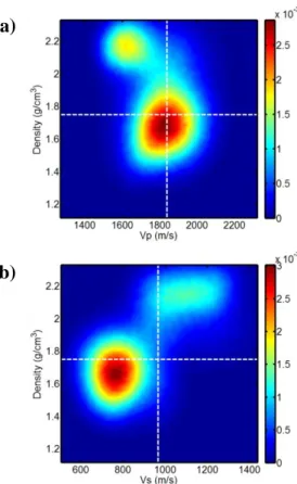
Figure 7 illustrates the posterior 2D marginal probability distributions estimated by the GA+GS 417
for the fourth layer. Figures 7a and 7b display the 2D distributions projected onto the Vp-density and Vs-density planes, respectively. The bimodality that characterizes the density PPD and the inverse correlation between the Vp and density parameters are both evident in Figure 7a.
22
Figure 7: The posterior 2D marginal distributions for the fourth layer. The Vp-density and Vs-density distributions are shown in a) and b), respectively. The dotted white lines represent the true 423
values. To better compare the resolution that is associated with each parameter, the axes are represented with the same scale.
426
The highest peak corresponds to a Vp of 1800 m/s and to a density of 1.7 g/cm³, which are very close to the true values (white dotted lines in the figure), whereas the secondary peak is located at lower Vp but at a higher density value, showing a negative Vp-density correlation. The higher 429
resolution that characterizes the Vp estimation with respect to the density estimation is also evident. The positive correlation between Vs and density clearly stands out when examining the Vs-density 2D marginal distribution (Figure 7b): in this case, higher density values are associated with higher 432
Vs values. The opposite parameter correlations that are shown in Figures 7a and 7b occur because we are trying to match not only the kinematics of the reflections but also their amplitudes. Concerning the amplitude of the reflections and considering the Aki and Richards equation (Aki 435
b) a)
23
and Richards, 1980) for the P-wave reflection coefficient from a single interface (or other analogous equations), the Vs and density contrasts exert an opposite influence on the variation in the reflection coefficient with incidence angle, while the Vp and density contrasts produce the same effects. Thus, 438
to keep the variation in the reflection coefficient constant with incidence angle, an increase in the Vs contrast must be associated with an increase in the density contrast; conversely, an increase in the Vp contrast must be associated with a decrease in the density contrast. Therefore, the GA+GS 441
method was also able to recover the correct correlations among the inverted parameters.
The proposed GA versus the standard GA implementation 444
To better illustrate the benefits in terms of the wider exploration of the model space that characterize the proposed GA implementation, we repeat the FWI test that was described in the previous section by using a standard, single-population GA. The main GA parameters (as the 447
individuals for each generation, or the maximum number of generations) are the same as those in the previous example. Due to the high-dimensional model space, we use the clustering technique that is known as self-organizing map (SOM; de Matos et al. 2006) to visualize the model space 450
explorations that are performed by the two different GA implementations. In particular, the entire set of GA models up to a given iteration will constitute the input ensemble for the SOM algorithm.
The SOM method uses a net that is formed by neurons to compute the unified distance matrix 453
(Ultsch, 1993), which is a 2D representation of a high-dimensional model space and helps to display clusters in high-dimensional spaces. In the following examples, we employ a particular version of the unified distance matrix, the so-called “sample hits” plot, which indicates how many 456
data points extracted from the input ensemble of explored models are associated with each neuron. Therefore, neurons associated with many data points can be thought of as a single cluster.
We aim to cluster the entire set of models generated up to a particular generation for the standard 459
GA and the proposed GA implementation. Models that explore the same portion of the model space will be classified by the SOM algorithm as belonging to the same cluster. To analyse the different
24
evolutions of the model space exploration, the SOM clustering is performed with the models that 462
were produced up to different generations serving as the input. The two examples start from the same initial random population and evolve for 40 generations. In Figure 8, the different explorations of the model space in the two cases are represented by the sample hits plot. In this case, we used an 465
8x8 map that consists of 64 neurons distributed according to a hexagonal topology. In Figure 8 the dimension of each violet hexagon is proportional to the number of input models that are associated with each neuron.
468
As expected, the distribution of the randomly generated models is fairly even in the initial generation (Figure 8a). However, comparing the evolutions of the two GA implementations after fifteen generations shows that the standard GA method has already restricted its exploration to 471
limited portions of the entire model space (Figure 8b), while the GA implementation we use is still exploring different sectors of the model space (Figure 8c). This characteristic of the standard GA method is confirmed at the last generation (Figure 8d), when most of the models generated during 474
the inversion are localized to a single restricted portion of the entire model space, evidencing the genetic drift effect. Conversely, the proposed GA implementation has performed a wider model space exploration as indicated by the many different clusters at the end of the 40 generations 477
25
Figure 8: Sample hits plots that represent the different evolutions of the standard single-480
population and our GA implementation. Each plot is generated by clustering the entire set of generated models up to a certain generation and projecting the result to a two-dimensional map (see the text for more details). The two tests start from the initial, randomly generated population of 483
models (a). The evolution of the standard single-population GA case is represented in b) and d), a)
b) c)
26
whereas c) and e) represent the evolution of our GA inversion. This figure demonstrates that the proposed GA implementation is characterized by a wider exploration of the model space compared 486
with the standard GA method.
Second synthetic example: underparameterization 489
Any attempt to exactly parameterize the subsurface will, in fact, be an underparameterization because the layers in real media are thinner and far more numerous than modelled layers (Sen and Stoffa, 1991). Starting from this basic knowledge, we consider a depth model that is derived from 492
actual well log data of Vp, Vs and density. In particular, by making use of the Backus averaging method (Backus, 1962) and considering a source wavelet with a dominant frequency of 50 Hz and the minimum velocity of the log, we scale the log data to the seismic scale by determining an 495
equivalent depth model with constant layer thicknesses of 3 m (Figure 9, black curves). On this scaled model, we computed a synthetic seismogram that constitutes our observed data.
In the following inversion, the forward modelling is performed by considering the same source 498
signature but with a dominant frequency of 15 Hz. Knowing that the expected maximum resolution of 1D FWI is between 1/4 and 1/6 of the maximum wavelength associated with the dominant frequency (Mallick and Dutta, 2002), we fix the layer thicknesses of the inverted model to 20 m, 501
that is, to 1/5 of the maximum wavelength. In the data misfit calculation, the modelled data are compared with a low-pass filtered version of the observed seismogram. In this example, the range of admissible values for Vp, Vs and density are set within ranges of 800 m/s and 0.8 g/cm3 for the
504
velocities and density, respectively (Figures 9a, b and c, grey lines), which are centred on heavily smoothed versions of the original logs. Both the GA setting and the seismic acquisition parameters are the same as those in the first example.
27
Figure 9: Comparison between the true (black) and the predicted (red) elastic properties (a, b and c). The black curves represent the log data after Backus averaging for a dominant frequency of 510
50 Hz. The red curves indicate the predicted elastic properties for a dominant frequency of 15 Hz. The grey lines show the inversion parameter ranges that have been defined around a highly smoothed version of the original log data.
513
The trends of the predicted properties (red lines in Figures 9a, b and c) reproduce the true elastic properties despite the different resolutions. As expected, the P-wave velocity shows a better match, 516
while the results are less accurate for Vs and particularly for density. The inversion was able to reconstruct the numerous sudden increases and reversals that occur in the true Vp profile. Figures 10a, b and c demonstrate the good fit between the observed and predicted seismic data in the 519
frequency bandwidth considered in the inversion.
28
Figure 10: a) Observed seismogram, b) best predicted seismogram and c) their difference for the 522
same frequency range during the inversion (which determines the layer thickness of the inverted model). The seismograms are NMO-corrected for the water velocity and are represented with the same amplitude scale.
525
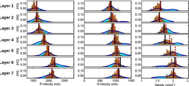
Figure 11 illustrates a comparison between the GA and GA+GS estimation of the marginal probability distributions for the first seven layers (excluding the water column, whose properties are 528
assumed to be known during the inversion). The conclusions that are drawn from the first example still remain valid in this more realistic test: the density remains the less-resolved elastic parameter and the GA method underestimates the uncertainty that is associated with each inverted parameter. 531
a)
b)
29
Figure 11: The GA approximation of the marginal PPDs (orange bars) and the final GA+GS estimation of the marginal distributions (cyan filled curves) are shown from top to bottom for the 534
first seven layers. The Vp, Vs and density values are represented in the left, central and right columns, respectively. The dashed red lines show the predicted model parameters by the GA inversion. To better display the variance of each parameter, the x axes are represented with the 537
same scale.
Third example: inversion of field data 540
Finally, we apply the hybrid GA+GS inversion to a field common shot from a marine well site survey, which is characterized by a 1 ms sampling interval, 20 m minimum offset, 12.5 m group interval, 607.5 m maximum source-receiver distance and 0.6 s recording length. The limited 543
maximum offset and the simple layered nature of the shallow strata make the assumption of a 1D model realistic. As for the previous synthetic example, we low-pass filter (0 – 37 Hz) the shot gather used in the inversion, yielding a vertical resolution of 20 m, which we fix as the thickness of 546
the layers in the inverted model. The source signature used in the inversion is taken from the recordings of an auxiliary channel that contains the source pulse for each shot. The GA setting is the same as that used in the previous tests, which results in a total number of individuals (that is, of the 549
30
The velocities that are determined from standard velocity analysis define the Vp trend, whereas the Vs and density trends are empirically scaled values from Vp, which are defined from the 552
lithological and geological context of the explored area (a shallow water shale-sand sequence). The admissible parameter ranges in the inversion are +/-300 m/s for Vp and Vs and +/-0.3 g/cm3 for density and are centred around their respective trends.
555
The results are illustrated in Figures 12a, b and c. We observe a linear and gradual increase for all the parameters and a significant Vp jump at 280 m, which is associated with a density decrease. We cannot be totally confident in the density estimates due to the ambiguities in the density 558
estimation and the cross-talk between velocity and density. Moreover, independent or additional data such as well log recordings or geotechnical data are not available to validate the results.
Figures 13a, b and c show the observed seismogram, the best predicted seismogram and their 561
difference, respectively. Given the noise contamination, the absence of any pre-processing and the elastic 1D assumption, the match between the predicted and observed data is reasonable. The evolutions of both the data misfit and the number of individuals for each subpopulation are depicted 564
in Figures 14a and 14b, respectively. Figure 14a shows that the trends of the different subpopulations nicely merge and assume a rather flat attitude after approximately 20/25 iterations, indicating that convergence has been attained. The evolution of the number of individuals for each 567
subpopulation is illustrated in Figure 14b. Figure 15 shows a comparison between the GA and GA+GS estimation of the marginal distributions for the first seven layers (excluding the water column, whose properties are assumed to be known). In contrast to the synthetic examples, the final 570
GA+GS marginal PPD estimations in this more challenging test appear more complex, and an increase in the uncertainties and ambiguities is visible for all parameters but is particularly evident for the density. The overall higher ambiguity in the parameter estimations may be ascribed to noise 573
contamination in the observed data but can also be due to the physical assumptions that were made in the forward modelling computation (e.g., perfectly elastic propagation, homogeneous and isotropic 1D media), which may not be totally verified in this specific case. Moreover, the very low 576
31
resolution that is associated with the density estimations is also related to the limited offset range that characterizes this WSS acquisition. However, for the purposes of this paper, this test confirms that the posterior marginal probabilities that are derived from the GA-sampled models strongly 579
underestimate the uncertainties that are associated with each inverted parameter and that the GS step is needed to better understand the true ambiguities that are associated with the final result.
582
Figure 12: The predicted model (red lines) and the admissible ranges for each parameter (grey lines) for the P-wave velocity, S-wave velocity and density in a, b and c, respectively.
32 585
Figure 13: The comparison between the observed and best predicted seismogram and their difference is shown for the same frequency range during the inversion (a, b and c, respectively). The seismograms are NMO-corrected for the water velocity and are represented with the same 588
amplitude scale.
591
Figure 14: The evolution of the data misfit and the number of individuals for each subpopulation (a and b, respectively).
a)
b)
c)
33 594
Figure 15: The GA approximation of the marginal PPDs (orange bars) and the final GA+GS estimation of the marginal distributions (cyan filled curves) are represented from top to bottom for 597
the first seven inverted layers. The Vp, Vs and density values are represented in the left, central and right columns, respectively. The dashed red lines show the best model parameters estimated by the GA inversion. To better illustrate the variance of each parameter, the x axes are represented with 600
the same scale.
Conclusions 603
We have described a hybrid method for uncertainty estimation that is applicable to stochastic inversions and combines the fast convergence of genetic algorithms with the accuracy of Gibbs sampler to estimate posterior probability distributions in model space. The first analytical test 606
showed that the true marginal and joint distributions of the considered variables cannot be estimated from the GA models alone because the GA optimization tends to oversample the model space regions that are characterized by lower data misfit (or higher likelihood), which results in a severe 609
underestimation of the uncertainties. A further refinement with a Gibbs sampler is needed to better estimate the uncertainties of the results and to correctly recover the correlation that exists among different inverted parameters.
34
Conclusions that are similar to those drawn from the analytical example can be derived from all the FWI tests on both synthetic and actual data: the validity of the hybrid GA+GS approach has been confirmed and its applicability to solving geophysical inverse problems has been positively 615
tested. As expected, the uncertainties increase when passing from Vp to Vs and density estimations. To avoid the overparametrization problem in the FWI inversion, we follow the approach proposed by Mallick and Dutta (2002) that fixes the layer thicknesses to a constant value of 618
between 1/4 and 1/6 of the maximum wavelength associated with the dominant frequency. We also attempted a peculiar implementation of the niched approach to GA’s to maximize the exploration of the model space and prevent the genetic drift effect. In particular, we applied different evolution 621
strategies to different subpopulations and employed tools such as the stretching of the fitness function, shrinking of the mutation range and competition between different subpopulations. By using the data from the first synthetic example and employing the SOM clustering technique, we 624
have demonstrated the improved model space exploration performance of our niched GA implementation compared to that of the standard, single population GA method. This advanced, niched GA inversion approach not only reduces the possibility of the genetic algorithm becoming 627
trapped in local minima but also performs a wider exploration of the model space, which is essential to ensure a reliable estimation of the posterior probability distributions in the successive GS step.
One limitation of the GA FWI lies in the high computational cost of the stochastic optimization 630
that, presently, makes unfeasible the applicability of the method to large, industrial scale, data volumes. However, we point out that a GA FWI is an embarrassingly parallel problem in which a large number of unrelated and independent forward problems can be solved sequentially with little 633
or no communication among different tasks. This makes it possible for a parallel implementation to greatly speed up the inversion. In this work we used a parallel genetic algorithm implemented through a Message Passing Interface (MPI) communication protocol. This parallel implementation 636
allowed the inversion of a single CMP gather of the field data to be completed in 6 hours, approximately. The GS algorithm is also easily parallelizable and less than half an hour was
35
required to complete this step for the field data test. These computational times refer to the use of a 639
Octave code running on 2 compute nodes of a Linux cluster in which each compute node is a 2 esa-core Intel(R) Xeon(R) CPU E5645 at 2.4 GHz. Therefore, there is room for significant improvements in the computational efficiency, for example by writing the code in a lower level 642
language, by optimizing its parallel implementation and by running the code on many more compute nodes.
Another limitation of the 1D FWI is the assumption of a 1D subsurface model that limits its 645
applicability to very simple geological contexts or to seismic data gathers that have been properly migrated (Mallick, 1999). However, despite this assumption and the high computational cost, the stochastic 1D FWI is a powerful method to derive elastic models of the subsurface that can be used 648
in many geophysical applications: e.g. well-site analysis, shallow hazard assessment (Mallick and Dutta, 2002) or reservoir characterization (Bacharach, 2006). Performing an extra Gibbs sampler step adds a negligible CPU time with respect to the GA FWI and yields valuable additional 651
information on the reliability of the estimations. Note that the uncertainties associated to the estimated elastic properties can be considered in subsequent investigations that make use of the GA FWI outcomes. In this sense, they can be propagated to further estimations such as porosity or 654
saturation estimations, to remain in a reservoir characterization context. The elastic properties estimated by 1D FWI, together with their associated posterior probability distributions, can be also useful for defining different initial starting models for local, gradient-based optimizations (Xia et al. 657
1998). We also point out that the uncertainty and the cross-talk that affect the final estimates, as seen in our examples, particularly the Vp-density cross-talk and the Vs and density uncertainties, can be greatly reduced if multicomponent seismic data or/and wide angle ranges (near or beyond 660
the critical angle) are available (Operto et al. 2013).
As a final remark, we point out that the GA+GS method in the present implementation can not be directly applied to 2D or 3D FWI due to unaffordable computational cost of the GA 663
36
quantification in 2D acoustic FWI. Our preliminary attempts indicate that it is crucial not only the availability of a highly efficient and parallel code running on tens of compute nodes, but more 666
importantly, an efficient strategy to reduce the number of inverted model parameters in the stochastic inversion.
37
APPENDIX A: A brief introduction to Bayesian inference and Monte Carlo integration The geophysical inversion problem of estimating earth model parameters from observations of 672
geophysical data often suffers from non-uniqueness, that is several models may fit the observations equally well. Casting an inverse problem in a statistical framework (Tarantola, 2005) allows us to characterize the non-uniqueness of the solution by its probability density function (PDF) in model 675
space. The main advantage of this approach lies in the fact that it produces the posterior probability density function for a model, given the observed data. Although most statistical approaches make simplistic assumptions of Gaussian prior PDFs and uncorrelated data errors, the results obtained 678
from such approaches are physically meaningful and with practical utility. In this section, we give a brief overview of the Bayesian formulation, following the concepts described in Sen and Stoffa (1996).
681
As usual, we represent the model by a vector m and the data by a vector d given by:
m1,m2, ,m
(A1) m= M T and 684
d1,d2, ,d
(A2) d = N Tconsisting of elements mi and di, respectively, where each element is considered to be a random
variable. The quantities M and N are the number of model parameters and data points, respectively, 687
and the superscript T represents a matrix transpose. Following Tarantola (2005) notation, we assume that p(d|m) is the PDF of d for a given m (also called the likelihood function), p(m|d) is the conditional PDF of m for a given d, p(d) is the PDF of data set d and p(m) is the PDF of model m 690
independent of the data. From the definition of the conditional probabilities, we have: ) 3 ( ) ( ) | ( ) ( ) | (m d p d p d m p m A p =
From this formulation we obtain an equation for the conditional PDF of model m given the 693
38 ) 4 ( ) ( ) ( ) | ( ) | ( A d p m p m d p d m p =
which describes the state of information for model m given the data d. This equation is the so-696
called Bayes' rule. The denominator p(d) does not depend on m and can be considered a constant factor in the inverse problem (Duijndam, 1988). Replacing the denominator in equation with a constant, we have: 699 ) 5 ( ) ( ) | ( ) | (m d p d m p m A p
The PDF p(m) is the probability of the model m, independent of the data, i.e. it describes the information for the model without any knowledge of the data and is called the prior PDF. Similarly, 702
the PDF p(m|d) is the state of information on model m given the data and is called the posterior PDF or the PPD. Obviously, the prior knowledge in the model is modified by the likelihood function, but assuming a uniform prior PDF, the posterior PDF is primarily determined by the 705
likelihood function (Duijndam, 1988). Assuming Gaussian errors (Sen and Stoffa, 1996), the likelihood function takes the following form:
( )
( 6) exp ) | (d m E m A p − 708where E(m) is a misfit function that we want to minimize in the inversion process. The expression for the PPD can thus be written as
( )
( ) ( 7) exp ) | (m d E m p m A p − 711This PPD is the final solution of the inversion problem from a Bayesian point of view. However, the PPD can not be displayed in a multi-dimensional space. Therefore, several measures of dispersion and marginal density functions can be used to describe the solution. Among these, the 714
marginal PPD of a particular model parameter, the mean model and the posterior model covariance matrix are, respectively, given by:
) 8 ( ) | ( ) | (m d dm1 dm2 dm 1 dm 1 dm p m d A p i =
i−
i+
M 717 ) 9 ( ) | (m d A p m dm m=
39 and ) 10 ( ) | ( ) ( ) (m m m m p m d A dm CM =
− − T 720Equations A8-A10 are often referred to as the Bayesian integrals and, for a non-linear inverse problem, they can be calculated via a numerical evaluation (see Sen and Stoffa, 1996; Sambridge, 1999). The generic Bayesian integral I, can be expressed as:
723
= dm f(m)P(m) (A11) I
where the domain of integration spans the entire model space and f(m) represents a generic function used to define each integrand. To simplify the notation, in equation A11 we substitute 726
p(m|d) with P(m) dropping the |d term. We maintain this notational simplification from here on. Using a Monte Carlo integration technique, a numerical approximation of equation A11 can be derived as follows: 729
= = N k k k k A m q m P m f N I 1 ) 12 ( ) ( ) ( ) ( 1where I indicates the numerical approximation of the Bayesian integrals, N is the number of Monte Carlo integration points and q(m) is their density distribution that is assumed to be 732 normalized: ) 13 ( 1 ) (m A q dm =
Equation A12 can be finally re-written as a simple weighted average over the ensemble of Monte 735
Carlo integration points:
= = N k k k w A m f N I 1 ) 14 ( ) ( 1where wk indicates the frequently called “important ratio” and is equal to:
738 ) 15 ( ) ( ) ( A m q m P w k k k =
40 741
APPENDIX B: Using the Gibbs sampler to approximate the Bayesian integrals
In the following we give a brief description of the GS step that constitutes the second part of the proposed methodology. We refer the reader to Sambridge (1999) for more detailed mathematical 744
information.
The GS algorithm exploits the finite ensemble of models collected during the GA optimization, and their associate likelihood, to refine the PPD estimated by the GA method. This can be viewed 747
as an interpolation problem in a multi-dimensional space (Sambridge, 1999). After performing a GA inversion, in which all the explored models and associated likelihoods have been saved and stored, the GA approximation of the PPD can be derived by constructing a multi-dimensional 750
interpolant using Voronoi cells in the model space (Voronoi 1908). This approximate PPD is derived by simply setting the known PPD of each model as a constant inside its Voronoi cell. We call this the GA approximation of the PPD, and write it as
753 ) 1 ( ) ( ) (m P m B PGA = iGA
where miGA is a model in the input ensemble of GA-sampled models that is closest to m (a
generic point in the model space). In particular, PGA(m)represents all information contained in the
756
input ensemble and constitutes the only information available in the GS step to compute the final PPD. If we assume an efficient exploration of the model space during the GA optimization, we can consider PGA(m) as a rough approximation of the target, final, PPD P(m). Then, we have:
759 ) 2 ( ) ( ) (m P m B PGA
This final PPD can be computed using a MCMC algorithm (such as the Gibbs sampler) that generates a new set of Monte Carlo samples (that will constitute the resampled ensemble) the 762
distribution of which asymptotically tends towards PGA(m). In other words, the new samples drawn during the GS walk are designed to importance sample the GA approximation of the PPD. The rejection method (Gilks and Wild, 1992) can be used to generate such resampled ensemble.