Alma Mater Studiorum
Alma Mater Studiorum –
– Università di Bologna
Università di Bologna
DOTTORATO DI RICERCA IN
Biodiversità ed Evoluzione
Ciclo XIII
Settore/i scientifico-disciplinare/i di afferenza: BIO 05 - ZOOLOGIA
TITOLO TESI
Population structure of aristeid shrimps (Decapoda,
Aristeidae) in the Western Mediterranean Sea inferred by
microsatellite loci
Presentata da: Flavio Sacco
Coordinatore Dottorato Relatore
Prof.ssa Barbara Mantovani Prof.ssa Barbara Mantovani
Index
1 Introduction2 Systematic,biology and management of the red and blue shrimp, Aristeus antennatus (Risso, 1816)
2.1. Classification and systematic 2.2. Morphology
2.3 Geographical and bathymetric distribution 2.4. Biological life cycle.
2.5. Feeding habits 2.6. Size and growth 2.7. Sex and reproduction
2.8. Evaluation and exploitation
2.9. State of resource and recommendations 3 Molecular Genetic Markers
3.1 Microsatellites
3.1.1 What are microsatellites? 3.1.2 Why choose microsatellites? 3.1.3 Drawbacks with microsatellites 4 Materials and Methods
4.1 Field collections
4.3 Microsatellite loci
4.3.1 Isolation of microsatellite nuclear markers 4.3.1.1 DNA preparation for enrichment 4.3.1.2 Enrichment
4.3.1.3 Cloning
4.3.2 Screening of colonies and amplification of inserts 4.3.3 Primers design and relative conditions
4.3.4 Amplification with cold and labelled primers
4.3.5 Analysis of fragments, sizing of alleles and assignment of genotype
4.3.6 Polymorphism and genetic indices of isolated loci 4.3.7 Population genetic structure and dynamics analyses
4.3.7.1 Population structure
4.3.7.2 Test for possible reductions or expansions in population size
4.3.8 Sex-biased Dispersal
4.3.9 Correction for multiple tests 5 Results
5.1 Isolation of nuclear microsatellite markers
5.2 Polymorphism and genetic indices of isolated loci 5.3 Population genetic structure and dynamics
5.3.1.1 Descriptive statistics
5.3.1.2 AMOVA, pairwise Fst and Bayesian approach 5.3.2 Growth and reduction of population size
5.4 Sex-biased dispersal
5.5 Comparing results with similar study on Aristaeomorpha foliacea 5.5.1 Isolation and characterization of microsatellite loci
5.5.2 Genetic population structure 5.5.3 Sex-biased dipersal
6 Discussion
6.1 Isolation of nuclear microsatellite markers
6.2 Polymorphism and genetic indices of isolated loci 6.3 Population genetics
6.4 Sex-biased Dispersal
6.5 Comparing results with similar study on Aristaeomorpha foliacea 7 Conclusions and Future studies
8 References 9 Annexes
1 Introduction
The red and blue shrimp Aristeus antennatus (Risso, 1816) is a species widely distributed throughout the world. It occurs in the Mediterranean, with a higher frequency in the western central part of the basin (SYNDEM, 1999), and off eastern Atlantic coasts from Portugal to the Cape Verde islands. In the western Mediterranean, the species is of great economic interest and, together with Aristaeomorpha foliacea (Risso, 1827), it is the main target species of deep-trawling, which goes up to 800-1000m (Demestre and Martìn, 1993; Ragonese and Bianchini, 1996; Sardà and Cartés, 1994, Matarrese et al., 1997, Cau et al., 2002). The exploitation of the red and blue shrimp in the eastern Mediterranean has not been increased yet, since, in that area, trawling cannot exceed the limit of 400-500m of depth (Politou et al., 1998). For this reason, in the eastern part of the Mediterranean Sea, Aristeus antennatus is considered practically unexploited (Papaconstantinou and Kapiris, 2001; Kapiris, 2004)!"
Today, main informations on A. antennatus derive from scientific researches supported by the economic interest of the species and in fact, data are mainly from the central part of the Mediterranean basin, where it is widely fished. This knowledge focuses on the biology, ecology, and fishing exploitation of the species.
Due to the “deep” biological habits of this species, aspects such as maximum depth of distribution, factors that influence the larval dispersal and ecology, and the population structure are poorly known.
The peculiar biological traits, the limited ecological knowledge and the strong exploitation pose several questions about the sustainability of current rates of
exploitation, threatening the long-term survival of this important commercial resource.
In fact, as in the case of several other marine species, the studies on the ecology of the species are overcome by the simultaneous exploitation of the species, and may not allow us to perceive the real impact that fishing has on populations of A. antennatus.
Among possible approaches, genetic studies may allow to gather thorough information in order to study biological, physiological and ecological aspects of the species. In particular, genetic data are extremely useful for the identification of "stocks" and gene flow dynamics.
The latest techniques in molecular biology may reveal important information about the distribution in Mediterranean of A. antennatus allowing, for example, to highlight the existence of genetically isolated populations of the blue and red shrimp.
Since direct tracking of individuals is very difficult for marine species, and even more challenging for deep-water shrimps such as A. antennatus, the use of indirect methods for the measurement of connectivity among populations is important (Cowen et al., 2007). Among the most recently developed indirect methods to infer connectivity, genetic approaches have been particularly successful (Hedgecock et al., 2007).
As mentioned before, information about the genetic structure and diversity of natural populations of A. antennatus throughout its natural range is very limited. Previous studies using either allozymes (Marchi et al., 1995; Pla et al., 1995; Sardà et al., 1998) or mtDNA markers (Maggio et al., 2009; Roldán et al., 2009; Sardà et al., 2010) have shown the absence of population differentiation. Genetic homogeneity of A. antennatus populations has been attributed to relatively recent separation in populations and/or ongoing gene flow, due to pelagic larvae dispersal, and adult migrations.
The use of more variable and polymorphic molecular markers, such as microsatellites (also known as simple sequence repeats, SSRs) could reveal the existence of genetically isolated populations, even if differentiation is very small, and populations are closely related (Wright and Bentzen, 1994).
In this study, the isolation and characterization of microsatellite loci for the red and blue shrimp are described for the first time and are applied in the study of genetic variation of A. Antennatus samples from nine different locations of the western Mediterranean area, in order to quantify the genetic diversity, analyze the genetic population structure and determine whether there are separate stocks of the species. Furthermore, due to different bathymetric distributions of the sexes and their possible differential dispersal capacity, we also tested the hypothesis of instantaneous sex-biased dispersal.
Finally, results are compared with those from a parallel PhD research project, developed with other fellows from the same institute, on Aristaeomorpha foliacea, analyzing differences and similarities between the two species.
Genetic information gathered in my study can provide important indications to be used on a scientific basis for regulating the exploitation of the resource, inaugurating a new course: Responsible and Aware Fisheries, that represent our primary goal. In fact, this PhD project was carried out at the Com.Bio.Ma., a centre of Competence on Marine Biodiversity, and funded by the “APQ RESEARCH – PROJECT P5 BIODIVERSITY” whose objectives are to realise laboratories on Marine Biodiversity, aimed to deepen knowledge on fishes and invertebrates from Sardinia.
"
2 Systematics, biology and management of the red and blue
shrimp, Aristeus antennatus (Risso, 1816)
2.1. Classification and systematics
!"#$%&'( #$%&$'(')*" )$*++'( +$,-%*./*" +%,)$*++'( 0*1*.'-%$*.*" -./0.'( 2/.*(')*" 1*&2$#'( #$3-%/3)*/" 304/0.'( !"#$%&'$( +!0)20+'( !"#$%&'$()*%&**)%'$(
The red and blue shrimp, Aristeus antennatus, is a deep-water shrimp from the Aristeidae family and together with Aritaeomorpha foliacea they are the only demersal Mediterranean species.
2.2. Morphology
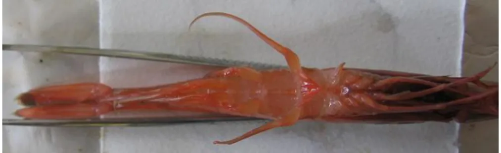
The red and blue shrimp, Aristeus antennatus (figure 2.1), is a big sized shrimp (maximum total length = 22cm), belonging to decapod crustaceans; adults present sexual dimorphism: males present a short rostrum, that overlaps the eye but not the distal end of the antennal scale (figure 2.2), while in females the rostrum is longer and sharp (figure 2.2). Nevertheless, sexually immature males present a rostrum as long in females (Mura and Cau, 1989). In both sexes, the rostrum presents three spines on the basal side. The carapace is not characterized by any hull neither empathic spine.
The red and blue shrimp main colour is pale red, often with bluish tones on the carapace.
Fig.2.2 Sexual dimorphism of the rostrum in A. Antennatus 2.3 Geographical and bathymetric distribution
Aristeus antennatus is found along meso-bathyal muddy bottoms, and mostly in the central part of the western Mediterranean (SYNDEM, 1999).
Fig.2.3 Aristeus antennatus geographical distribution in the Mediterranean Sea In Italian seas the geographical distribution of the species is quite irregular. A. antennatus is completely absent in the northern and central Adriatic sea and very rare in the its southern basin (Vaccarella et al., 1986). The blue and red shrimp is abundant in the Ionian Sea, Tyrrhenian Sea, but for its southern part (AA.VV., 1990), Ligurian Sea, in the Strait of Sicily and along the south-western coasts of Sardinia (SYNDEM, 1999).
Male rostrum Female rostrum
A. antennatus is also found along the eastern side of Corsica, even if in lower concentration than the giant red shrimp A. foliacea (Campillo, 1994). Generally, the red and blue shrimp is found in deep waters, deeper than 400m , and it is the species with the widest depth distribution in the Mediterranean Sea. It occurs over muddy bottoms of the slope between 80 m (Nouar, 2001) and 3300 m (Sardà et al., 2004). Different authors have observed vertical migrations to shallower waters during nighttime (Campillo, 1994; Matarrese et al., 1995). Such events are mainly observable near to the edges and apices of underwater canyons. The depth distribution seems to influence also the sex-ratio of the species, which is biased towards females between 400 and 700m of depth as reported by different authors in different seas (Orsi Relini, 1980; Mura and Cau, 1989; Ragonese et al., 1996; Matarrese et al., 1995; Spedicato et al., 1995). On the other side, males seem to be more abundant than females between 1000 and 2200m of depth (Sardà et al., 1994). 2.4. Life cycle
The red and blue shrimp, directly disperse the eggs in the water column, where they hatch, starting a complex biological cycle (figure 2.4). Eggs free a very simple and little larvae: the nauplius, the first of 11 probable larval stages which include 5 nauplius stages, 3 protozoae stages and finally 3 mysis stages. A. antennatus larvae have been found only four times (Heldt, 1954; 1955; Seridji, 1971; Dos Santos, 1998; Carbonell et al., 2010) and always in the upper water layers, far from the adult fishing grounds where they should have originated (Carbonell et al., 2010). It is likely that newly hatched larvae perform a rapid and long vertical migration from the deeper spawning areas to the upper layers, where the subsequent stages develop, passively transported by the superficial currents (Carbonell et al., 2010). During the early stages, larvae are transported near to the coast. Here, after the larval phase, the individual becomes a postlarva and settles on bottoms, changing its habits: from planktonic to benthic. This usually takes place 3 weeks after the egg has hatched. Another major ontogenetic migration takes place when the post-larva moves to deeper waters becoming young recruits and later adults. These can reproduce and
start a new biological cycle. Usually the “new comers” reach these reproductive grounds when they are about one year old (FAO, 1987).
2.5. Feeding habits
The red and blue shrimp shows, as described in Brian (1931) and Lagardère (1972), a euriphagous behaviour. Its diet includes organisms preyed on the bottom like worms, echinoderms, the decapod Calocaris macandreae, small bivalves, gastropods and crustaceans belonging to various groups, and also euribathyc micro-nekton organisms, in particular Eufausiacea and Decapoda (Relini and Orsi Relini, 1987). If we consider the total number of prey, the 50% of them are crustaceans (Cartés and Sardà, 1989). Nevertheless, considering not only the number but also the size of prey, pelagic decapods as Sergestidae, Pasiphaeidae e Oplophoridae assume a fundamental role in the diet (Orsi Relini et al., 1995).
2.6. Size and growth Size
The maximum carapace length (LC) observed for females and for males resulted 71mm and 40mm, respectively, in samples from the Ligurian Sea (Orsi Relini and Pestarino, 1981; Orsi Relini and Relini, 1996).
Growth
The estimated growth parameters show adaptation to two different scenarios, either of “slow” or “fast” growth (Ragonese and Bianchini, 1996). Actually, literature data (table 2.I) seem to agree in attributing slow growth and a longer life span to females (6-10 years; Orsi Relini and Relini, 1996; 1998).
Tab 2.I Growth parameters for Aristeus antennatus where, L!, maximum theoretical length, K/year, slope; t0, age at size zero.
AUTHOR AREA SEX L! (mm) K/year t0
Orsi Relini et al.,
1996/98 Ligurian Sea F 71.2 76.9 0.317 0.213 -0.047 -0.019 Spedicato et al., 1995 Central-southern Tyrrhenian Sea F 66.81 0.558 -0.2337
Arculeo et al., 1994 Southern Tyrrhenian
Sea F 69.4 0.337
Cau et al., 1994 Sardinian Seas F 76.8 0.34 0.369
Colloca et al., 1998 Central Tyrrhenian Sea F 67.65 0.49 0
Ragonese and
Bianchini, 1996 Strait of Sicily F 69.1 0.532 0
Matarrese et al.,
2.7. Sex and reproduction
A. antennatus is a gonochoric species; the breeding season begins in spring, in April, with peaks in summer, when most of the females reach sexual maturity, and ends in autumn, during the months of October-November (Demestre , 1995).
Females and males can be distinguished even in the juvenile stage due to the different location and morphology of the gonads and to the presence of secondary sexual characteristics. Females have an open thelycum structure. This small cavity, appointed to host the male spermatophores (figure 2.5) is located between the third pair of pereiopods.
Fig 2.5 Female specimen of A. antennatus, with a male’s spermatophore.
In males, the basal part (endopodite) of the first pair of pleopods are transformed into a laminar structure (figure 2.6), the so called petasm, by which the spermatophores are transferred to the female thelycum. In young individuals this structure is split in two halves.
In A. antennatus, thelycum and petasma seem to act in a synchronous manner during mating, carrying and supporting spermatophores before fertilization, which thus takes place in the absence of the male (Demestre and Fortuno, 1992). This strategy can be beneficial for species such as A. antennatus showing a gender-segregation and/or a depth range that allows little contact between males and females (Sardà et al., 1997). In species with this anatomical morphology, spermatophores are transferred during an inter-moult period. For the blue and red shrimp it has been suggested a possible a repetition of the sequence moult-mating-moult for several times during the same breeding season.
Four ovarian maturation stages have been described: they can be recognized using a macroscopic colour scale (Orsi Relini, 1980). Ovaries in immature females or in post-spawning are colourless or white (stage 1). With the progression of vitellogenesis and the inclusion of caroteneprotein, the ovaries first are stained pink (stage 2) and then lilac (stage 3, advanced maturation stage, oocytes up to 250 "m). At the final stage of development the gonad appears of a dark purple colour (stage 4, oocyte diameter about 300 "m).
In males, a two-stage spermatogenesis has been identified through macroscopic surveys. The young male (stage 1) has a white deferent vessel without spermatophores and emipetasms are separated. Mature males (stage 2) have spermatophores and emipetasms appear joined (Demestre and Fortuno, 1992).
Before sexual maturity, at the beginning of the breeding season, females are bigger in size. With the progress of the breeding season, the average size of first sexual maturity tends to decrease, but increases again at the end of the period (Mura et al, 1992; D'Onghia et al., 1997).
In males, the reproductive phase seems to be more extended, in fact mature males with emispermatophores in the terminal portion of the sperm ducts have been
observed even in fall and winter (Orsi Relini and Pestarino, 1981; D'Onghia et al., 1997).
2.8. Evaluation and exploitation
Indices of abundance for A. antennatus, (table 2.II) referred to the trawl-survey MEDITS-95, appear to be for the layer 200-800 m higher in the Ionian, Ligurian and Sardinian Seas.
Tab.2.II Indices of abundance for A. antennatus, where: kg/km2, biomass index, CV, variation coefficient.
Parameters of total and natural mortality, estimated for some Italian waters for female of Aristeus antennatus, are shown in table 2. III.
INVESTIGATED AREA LAYER 200-800 M
kg/km2 CV
Ligurian Sea 4,46 44,05
Northern Tyrrhenian Sea 0,08 95,33
Central Tyrrhenian Sea 0,12 72,7
Southern Tyrrhenian Sea 0,78 61,31
Sardinian Seas 4,2 35,59
Strait of Sicily 0,46 53,43
Tab.2.III Mortality rates for Aristeus antennatus where M, natural mortality rate, Z, total mortality rate.
A. antennatus is an economically important resource: in the Ligurian Sea (Orsi Relini and Relini, 1985), in the Tyrrhenian Sea (Mailloux and Lembo, in AA.VV., 1990; Arculeo et al., 1994; Ardizzone et al., 1994), in the seas of Sardinia (Mura et al., 1992), in the Strait of Sicily (Ragonese and Bianchini, 1996) and in the Ionian Sea (Matarrese et al., 1992).
Despite the blue and red shrimp is subject to high fishing pressure, it is believed that this resource is currently submitted to a sustainable harvest rate (SYNDEM, 1999). The ability to maintain such levels of exploitation seems to be linked to the extremely broad distribution on bathyal bottoms of the species (Bianchini and Ragonese, 1994), and to the partial vulnerability of A. antennatus stocks, since only a fraction of the stock is accessible for commercial fishing fleets (Demestre and Lleonard, 1993). However, the application of “yield per recruit” models showed an overfishing condition (Mailloux et al., 1995). Also in the Ligurian Sea, the trends of the commercial landings are in decline (Fiorentino et al., 1995). Although it is possible that this resource is currently in a downturn in fluctuation cycle (Caddy, 1993), a
AUTHOR AREA SEX M Z
Spedicato et al., 1995 Central-southern Tyrrhenian Sea F 0.583-0.695 1.937-1.962
Cau et al., 1994 Sardinian Seas F 0.46
Ragonese and
Bianchini, 1996 Strait of Sicily F 0.8 1.1
Matarrese et al.,
more conservative management may be advisable. The fishing yields of blue and red shrimp are nonetheless subject to seasonal variations and annual fluctuations.
In fact, catches of this shrimp are known to fluctuate considerably from year to year, and recent studies have demonstrated the existence of a relationship between environmental factors (e.g., marine currents, water masses, and climate variability) and abundance fluctuations of A. antennatus (Cartés et al., 2008; Company et al., 2008; Guijarro et al., 2008; Massuti et al., 2008; Maynou, 2008a; b; Cartés et al., 2009). In particular, higher landings have been recorded 2-5 years after particularly cold winters and negative North Atlantic Oscillation index (NAO) periods. This pattern is likely due to the increased dense shelf water formation, with the cascading of superficial water masses that propagate along and across the continental slope. The transportation of particulate organic matter to the deep basin determines higher macrobenthos production, higher prey availability, and consequently higher fecundity. The enhancement of recruitment of A. antennatus could be also due to higher larval survival resulting from increased food availability and to the decrease of predation pressure due to the turbidity anomalies generated in the deep layers after cascading events (Company et al., 2008).
2.9. State of resource and recommendations
An increase in the size of recruits, by adopting a more selective mesh, will lead to future increases in productivity, thus leading to a less serious condition of exploitation without economic repercussions in the short term (Ragonese and Bianchini, 1996) .
Moreover, for Ionian Sea a period of fishing closure during the late summer, is recommended to reduce the fishing pressure on the recruits, particularly vulnerable during this period (D'Onghia et al., 1997).
3 Molecular Genetic Markers
The main instruments used to study the genetic variability within or between populations and species are genetic markers. A genetic marker is any morphological, biochemical or molecular character that is inherited through generations, so that they can be monitored over time (Brooke, 1999).
Genetic markers are used in a multitude of applications in the study of ecology and evolution (mating models, population structure and gene flow, fitness, etc.).
In recent years, scientists using a 'molecular approach' in population-based studies may apply a wide range of methodologies of analysis: this is because the continuous discovery and development of investigative techniques increasingly sophisticated does never completely replace the older ones. Further, many markers for the direct study of the DNA (RAPD, RFLP, AFLP, minisatellites and microsatellites) and markers for the study of its products (Allozyme) differ in the kind and degree of variability which they identify, in the ease of employment, and last but not least, costs of development and application (Ouborg et al., 1999).
Analysis conducted with allozymatic markers, though, are nowadays less and less used, as the allozymes (enzymes encoded by different alleles of a single locus, with different electrophoretic mobility due to alterations in the overall ionic charge of the protein) can be considered as indirect indicators of genetic variability. They are not able to detect modifications in the DNA that do not involve changes in the ionic charge and thus the overall protein mobility in an electric field.
A molecular marker has to be selectively neutral and basically must follow the Mendelian principles to be used as a tool to reveal the demographic pattern.
Among the many features that differentiate one molecular marker from the other, three aspects in particular should be highlighted:
! +,-#*)*.&(/(0,1,-#*)*.&(
Dominant markers (e.g. RAPD, AFLP) are those in which one allele is dominant on the other and the heterozygote profile is essentially indistinguishable from dominant homozygote. For this reason it can recognize only two phenotypes, dominant or recessive.
Codominant markers (RFLP, allozyme, microsatellites), instead, are those whose homozygous profiles can be distinguished from the heterozygous profile allowing precise estimation of allele frequencies in a population.
! 2*3&"#%)*.&(."#%&"#,*"
Markers differ in their criterion of inheritance: the nuclear DNA is inherited from both parents, while the DNA of organelles (mitochondrion and chloroplast) has more often a uniparental inheritance.
! 4&*&%#.(5)"#)6#7#%8(
Finally, in a gonochoric situation, owing to amphimixis, the nuclear genome of the new individual takes origin from the contribution of two parents allowing genetic variability, while the DNA of organelles in general doesn’t, as it is uniparentally inherited.
The degree of variation that a marker must have depends on the specific question to which you want to answer and also on the type of populations and organisms you want to study.
In this particular study I decided to conduct an analysis of the genetic variability of Aristeus antennatus at the nuclear level using microsatellites which are codominant and biparental inherited markers.
Animals nuclear DNA is a diploid genome transmitted according to Mendelian segregation and it is subject to recombination. Its more polymorphic regions, microsatellite loci, originally studied in relation to genetic diseases, are highly informative in population structure and dynamics studies (De-Xing Zhang and Godfrey M. Hewitt, 2003). Their high variability is due to the fact that these portions are not coding, and therefore not subject to selection.
3.1.1 What are microsatellites?
Microsatellites are high-frequency repeats of 1-6 nucleotides modules found in the nuclear genome of many taxa. They are also known as simple sequence repeats (SSR), variable number of tandem repeats (VNTR) and short tandem repeats (STR).
Fig.3.1 Schematic representation of a microsatellite with reported aside a few sequence examples.
Our understanding on the behaviour microsatellites in terms of mutation, function, evolution and distribution in the genome and across taxa is rapidly increasing (Li et al., 2002; Ellegren, 2004).
A microsatellite locus typically ranges in length from 5 to 40 repetitions, but longer repeats are possible. Typical microsatellites widely chosen for molecular genetic studies are those made of dinucleotides, trinucleotides and tetranucleotide. It should be noted that the trinucleotides (and also esanucleotides) can occur in coding
sequences since they do not cause the frameshift of the sequence (shift of the sequence that totally changes the reading of the triplets by the ribosome).
Sequences of DNA around the microsatellite locus are known as “flanking regions”. Since these flanking regions are conserved in different individuals of the same species, and sometimes even between related species, a microsatellite locus can be identified by its flanking regions on which primers can be designed to allow the specific amplification of the microsatellite locus.
Many microsatellites have a very high mutation rate, between 10-2 and 10-6 mutations
per locus per generation and an average of 5 x 10⁻⁴, which creates a high level of allelic diversity necessary for genetic studies (Schlotterer, 2000).
Microsatellite repeat sequences frequently change due to errors during DNA replication, primarily by changing the number of repetitions of the sequence (Eisen, 1999). Because the alleles differ in length, they can be distinguished by high resolution electrophoresis gel, allowing rapid genotyping of many individuals for several loci.
3.1.2 Why choose microsatellites?
Many issues in molecular ecological studies are discussed with more than one marker. Microsatellites are of particular interest because they allow researchers to deepen into complex ecological questions.
Ease of sample preparation.
An ideal marker requires small tissue samples that can be easily stored for future use. In contrast with methods based on allozymes, DNA-based techniques, just as microsatellite, use PCR to amplify markers from very small portions of sample. The stability of DNA is another big advantage over enzymes, as this allows the use of simple substances and reagents for the tissue preservation. Moreover, microsatellite sequences are usually short (100-300bp) and can almost always be amplified, despite the possible degradation of DNA (Taberlet et al, 1999). This feature of
microsatellites allows easy and economic DNA extraction even from ancient DNA, from hair and faecal samples used in non-invasive sampling (Taberlet et al., 1999). Finally, microsatellites, being species-specific, present no risk of cross contamination from other non-target organisms, which, can occur with other techniques employing universal primers (e.g. AFLP).
Highly informative content.
Each genomic locus can be considered as a representative sample for its genome, but, given that the different evolutionary events (recombination, mutation, genetic drift, selection) does not affect all loci equally, an investigation cannot be based on a single locus which could lead to high error rates in assessments. So taking advantage of many loci, as in the case of studies with microsatellites, allows us to perform multiple sampling of the genome with the possibility of crossing the results and get a broader picture of the situation. Although techniques such as AFLP, allozyme and RAPDs are considered multi locus, these do not have the same resolving power of microsatellites (Sunnucks, 2000). F.e., Gerber et al. (2000) demonstrated that 159 AFLP loci revealed even a lower resolution than six polymorphic microsatellite loci in determining paternity.
Microsatellites, due to their high mutation rate, are useful in studies involving the actual demography, the connection structures, determination of changes in the recent past (10-100 generations), studies of population structure and migration (Kalinowsky, 2002, Wilson and Rannala, 2003).
3.1.3 Drawbacks with microsatellites
Despite many advantages, microsatellites exhibit also many difficulties and problems that can complicate the data analysis, and even restrict their use or make the results very cryptic.
Primers amplifying regions common to many species (such as 12S, D-loop and others) and used in most molecular studies, are usually highly conserved sequences within the species and sometimes across taxonomic groups. This high conservation in the sequence involves many difficulties in optimizing the use of these primers when widening the analysis to new species.
In contrast, a couple of primers for a microsatellite locus rarely works in different taxonomic groups, and so primers have to be designed ex-novo for each new species that is studied (Glenn and Schabl, 2005). Today, isolation of new microsatellite markers is cheap and fast, although it has still a significant failure rate, especially in certain marine invertebrates (e.g. Cruz et al., 2005), Lepidoptera (Meglecz et al., 2004) and birds (Primmer et al., 1997).
Unclear mutational mechanisms
Microsatellite mutation model appears to be complex and, fortunately for most ecological applications is does not seem important to know the exact mutation mechanism at each locus, because this kind of analyses is insensitive to these mechanisms (Neigel, 1997) even if we can find methods based on the estimation of allele frequency using an explicit mutation model.
To date, four different models have been proposed to explain the evolution of microsatellite loci, i.e. the origin of new alleles: IAM (Infinite Alleles Model; Kimura and Crown, 1964), SMM (Stepwise Mutation Model; Kimura and Ohta, 1978); KAM (K-Allele Model; Crown and Kimura, 1970) and TPM (Two-Phase Model; Di Rienzo et al., 1994). Between these, It is to be noted that the first two models are more extreme, while the others represent variants of the firsts.
Traditionally, in population genetic analysis, we use the infinite allele model, IAM, (Di Rienzo et al., 1994). According to his model, mutations occurring in microsatellites involve the loss or the gain of one or more repeats simultaneously and lead to the formation of a new allele never met before in the population. F statistic is
based on this model which is also still the most popular one because it appears to be the simplest and generic model.
The other principal specific model for microsatellites, the stepwise mutation model, SMM, (Di Rienzo et al., 1994), assumes that mutations lead to loose or acquire only one repeat at a time at a constant rate, mimicking the replication errors in the polymerase that generate mutations, creating a Gaussian type of allele (Ellegren, 2004). Under these conditions, the more two alleles differ in size, the more they can be considered divergent from a common ancestor. R statistic is based on this model. But we must also remember that non-staged mutations occur, including point mutations or recombinant events such as gene conversion and unequal crossovers (Richard and Paques, 2000). Gradualism seems to be predominant in the microsatellite mutational events, but a more complex model that would include both gradual and non-staged events could better explain the mutation dynamics of such loci.
The allelic identification based on sizes in the microsatellite genotyping appears to be a good shortcut compared to the sequencing of each individual; however, it assumes that all alleles differ only in length and the ones that exhibit sequence differences but same length, will then be considered equal. This phenomenon is called "homoplasy", which can be revealed if it is subsequently highlighted by sequencing the alleles, or undetectable when two alleles have the same sequence but different genealogical histories. This non-identity is found in the gradual mutation behavior when there is a reverse mutation or the allele is different from its counterpart and then returns to original form. The homoplasy can finally concern the flanking regions, because the mutation can occur in this stretch, leaving unchanged the size of microsatellite allele. Amplification issues
Finding a good locus marker for DNA implies to find a region of the genome that has a mutation rate high enough to produce multiple versions of the locus, alleles, in the
same population, flanked by highly conserved regions on the other side, over which the PCR primers anneal in almost all individuals of the species (about 99-100%). In fact, if there are mutations in the flanking regions, some individuals will have only one allele amplified or even none.
It was found that some taxa appear to be more afflicted by amplification problems than others, as in the case of molluscs, corals and other invertebrates.
Despite the problems listed above, the versatility of microsatellites overcomes these drawbacks by far. Also, fortunately, many of these problems can be avoided through careful selection of loci during the process of isolation.
4 Materials and Methods
4.1 Field collections
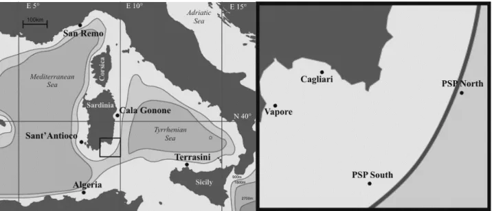
Individuals of A. antennatus analyzed in this study come from nine sampling areas of the western Mediterranean basin: Algeria, San Remo, Cala Gonone (Sardinia EC), Sant’Antioco (Sardinia SW), Gulf of Cagliari (Sardinia S), Vapore (S Sardinia), Terrasini (NW Sicily) and a site called PSP, which covers a south-east area of Sardinian sea (table 4.I and figure 4.1). Individuals were collected in 2006–2008 using both commercial bottom trawling (# 800 m depth) and experimental deep bottom trawling (from 800 to 1600 m). In the latter instance, individuals named PSP come from two different experimental deep fishing trawls, conducted by the Department of Animal Biology and Ecology, University of Cagliari. PSP South and PSP North are the only localities for which two different temporal replicates (2006 and 2007) were collected (table 4.I, figure 4.1).
Tab.4.I Location, year of sampling, depth of capture, number, and sex of individuals of each sample analyzed. Individuals from commercial hauls (*) were presumably caught at 800 m depth or shallower. The sex of the individuals from Algeria, San Remo, and Terrasini is unknown (ND = not determined) because only pereiopods were available for the genetic analyses. PSP (Pesca-Profonda-Sperimentale) indicates the experimental hauls.
Sampling locations Year of sampling Depth in m mean (max)
N of individuals (males, females)
Algeria 2006 <800 * 20 (NA)
San Remo 2007 <800 * 29 (NA)
Cala Gonone 2007 <800 * 20 (0,20) Terrasini 2007 <800 * 20 (NA) PSP North 2006, 1507 (1621) 12 (4,8) PSP North 2007 1421 (1422) 12 (1/11) Sant’Antioco 2007 <800 * 26 (6,20) Cagliari 2006 <800 * 17 (0,17) PSP South 2006 1117 (1227) 29 (22,7) PSP South 2007 1110 (1173) 26 (21,5) Vapore 2008 <800 * 16 (16,0) Total 227
Fig. 4.1 Map of the sampling sites. The right square represents an enlargement of the Gulf of Cagliari.
4.2 Tissue sampling and DNA Extraction
Muscle tissue was sampled from pereiopods or tails and preserved in 70–100% ethanol at 4 °C. Total DNA was extracted from tissue (5-10 mg), following “Salting Out” extraction protocol (Miller et al., 1988),with minor modifications. This protocol provides protein precipitation and their removal from aqueous solution containing the DNA, according to the principle of variation of ionic strength due to the addition of a salt, in this case NaCl> 6M: added salt ions compete with the ions in the solution facilitating protein aggregation.
The extracted DNA was eluted in 50 "l of sterile ddH2O. Quality and quantity of
isolated DNA were verified by electrophoresis in agarose gel 1%, in TAE 1X Buffer (BIO-RAD), at 70V for 15 minutes (figure 4.2).
Fig.4.2 Control of DNA extracted from various samples on 1% agarose gel.
4.3 Microsatellite loci
4.3.1 Isolation of microsatellite nuclear markers
Isolation of microsatellite markers has been done using the FIASCO protocol - Fast Isolation by AFLP of Sequences COntaining repeats - (Zane et al., 2002) with minor modifications. This allowed the construction of a partial genomic library enriched for AC repeat.
The protocol is part of recent isolation protocols through selective hybridization using biotinylated probes. It can be schematically divided into three phases (figure 4.3): 1. PREPARATION FOR ENRICHMENT;
2. ENRICHMENT; 3. CLONING.
4.3.1.1 DNA preparation for enrichment
A genomic DNA mix from 5 different individuals of Aristeus antennatus from the sample PSP South was digested with restriction MseI (Invitrogen) and contemporaneously ligated with MseI adaptors used for the AFLP procedure (Vos et al., 1995), as follows:
- Genomic DNA 25-250 ng;
- Buffer OnePhorAll 1X (Pharmacia); - DTT 5mM
- BSA 50 µg/ml - Adaptors 1 µM - ATP 200 µM - MseI 2,5 unità
- T4 DNA ligase 1 unit
__________________________
Total volume of reaction: 25 µl
The reaction mix has been incubated for 3 hours at 37°C.
The DNA fragments ligated to adapters were amplified using PCR (figure 4.4) .
DNA from the ligation reaction for was not diluted (1:10) following protocol, but the restricted-ligated DNA was used as template, along with four AFLP primers specific for the adaptors. The primers differ in the terminal base at the 3 'end (A or C or G or T).
The amplification mixture was as follows: - non diluted restriction-ligation reaction 5 µl - Buffer 1X
- MgCl2 1,5 mM
- primer 1,5 ng/µl each - dNTP 200 µM
- Taq DNA polymerase 0,4 unit __________________________ Total volume of reaction: 20 µl
The amplification reaction was performed in an Invitrogen thermocycler, with the following temperature profile:
Initial denaturation 94°C 2' Denaturation 94°C 30'' Annealing 53°C 1' Extension 72°C 1' 22 cycles Final extension 72°C 5'
Fragments obtained with PCR conditions adopted above, are typically sized between 200 and 600 bp and visible on agarose gel as a smear (figure 4.5).
The PCR reaction was replicated twenty times in order to have several hundreds nanograms of amplified product, enough for the following enrichment step.
Fig.4.4 Preparation for enrichment: restriction-ligation and amplification of restricted-ligated DNA.
Fig.4.5 Control of restricted-ligated amplification on a 1,8% agarose gel
4.3.1.2 Enrichment Hybridization
DNA hybridization was carried out with a 5' end biotinylated (AC)17 probe.
Hybridization was performed in 100 µl of 6X SSC / 0.07% SDS, mixing 200-300 ng of purified restricted-ligated DNA with 50-80 pmol of the probe, heating at 95 ° C for 3' and letting slowly cool to room temperature.
The solution was diluted with 300 µl of TEN100 (10 mM Tris-HCl, 1 mM EDTA, 100 mM NaCl, pH 7.5).
Selection of hybridized DNA using streptavidin paramagnetic spherules
Probe hybridized DNA was selected with the use of streptavidin paramagnetic spherules (Streptavidin Magnetic Particles, Roche; 1 mg per reaction). The streptavidin binds irreversibly to the biotin and, being associated with paramagnetic spherules, it can be removed from the solution by applying a magnetic field generated in this case by a special eppendorf tubes magnetic rack (Magnetic Rack, Invitrogen). The magnetic spherules were prepared by treating them with 2-3 TEN100 washes, each 5' long, at room temperature. After mixing 100 µl of hybridized DNA with 300 µl of TEN100, 5 "l of tRNA (10 mg / ml) and 50 µl of previously prepared spherules, everything was incubated at 50°C for 30'.
Definitive removal of non hybridized DNA
In order to remove the DNA not linked to the probe, three not stringent washes (400 µl of TEN100) and three stringent washes(400 µl of 0.2 X SSC buffer and 0.1% SDS) were performed. After each wash, 5' long at room temperature, shaking gently the solution, the hybridized DNA was removed using the magnetic field and the washing solution was discarded.
To separate the enriched DNA from the biotinylated probe-magnetic spherules complex, the mixture has been subjected to two denaturing steps:
• 1st Denaturation: 95°C for 5' with 50µl of TE 10:1 (Tris 10 mM, EDTA 1 mM), pH 8 (the supernatant containing the DNA of interest was quickly removed and stored);
• 2nd Denaturation: the pellet from the first denaturation was incubated 5' at room temperature with 20µl of TE 10:1, 8µl of 0.15 M NaOH/acetic acid 0.166 M pH 7.
The DNA from the 2 denaturation steps was stored for the next step: the volume of the eluate was measured and the DNA was precipitated with an equal volume of isopropanol and sodium acetate (final concentration 0.15 M).
Finally, I carried out the control of the two previous denaturation steps and of the three washes on an 1,8% agarose gel (figure 4.6).
Amplification of enriched DNA
The enriched DNA obtained from the first and the second denaturation steps was precipitated with 85% ethanol and resuspended in 50µl of sterile water; 2µl were amplified for 30 cycles using AFLP primers specific for the adapter under conditions described in “DNA preparation for enrichment”.
Fig.4.6 Control of denaturations and washes of enriched DNA
L1 = contains tRNA, which works as a carrier for RNA, taking it away with it. Smear hasto be focused under 300bp.
L2 = Represents DNA not ligated to the probe. L3 = Represents DNA not ligated to the probe.
D1(4) = Microsatellite-enriched DNA separated from the probe. D2 (5) = Microsatellite-enriched DNA separated from the probe. DNA concentration is lower, but its quality higher.
L100 = Ladder 100 bp 4.3.1.3 Cloning
The microsatellite-enriched DNA has been cloned (figure4.7) with the TOPO TA CLONING® kit (Invitrogen) containing Escherichia coli cells and the plasmid vector pCR®II-TOPO®.
This vector is characterized by a dominant selective marker for resistance to ampicillin and it is linearizedwith3'desossitimidineresidues to which Topo isomerise I is covalently linked. This (with the addition of the non-specific Taq polymerase with terminal transferase activity) allows the microsatellite- enriched DNA - PCR produced - to bind efficiently the carrier thanks to the presence of a 3'desossiadenine (figure 4.8).
Fig. 4.7 Cloning of DNA
Fig.4.8 pCR®II-TOPO® vector of the cloning kit TOPO TA CLONING® (Invitrogen).
Ligation reaction
In a total volume of 6µl, 1µl of DNA (PCR product) was mixed with 1µl of saline
The solution was mixed gently and incubated for 5'at room temperature, then placed on ice.
Transformation
Two µl of the previous reaction (TOPO cloning reaction) were added into a tube containing cells of Escherichia coli. To allow cell transformation the mix was incubated on ice for 30' then subjected to heat shock at 42°C
for 30'' and placed back on ice. We proceeded with the addition of 250µl of SOC cells, and gently mixed the tube at an oblique position for 1h at 37°C. In the meantime, culture plates were prepared with Luria-Bertani solid medium (1% Tryptone, 0.5% yeast extract, 1% NaCl, pH 7, 15 g/L agar), 50g/ml ampicillin and 40µl of X-Gal 40mg/ml (beta-galactosidase substrate).
Cell seeding and cell growth
Transformed cells were plated at different volumes (100, 75, 50 and 25µl) to obtain, at least for one plate, spread of colonies that would facilitate the withdrawal (figure 4.9). The plates were incubated overnight at 37°C. After cells of E. coli raised to colonies on the plates with solid medium, we proceeded to the selection of those containing the insert, on a colorimetric basis thanks to the X-Gal reaction (figure 4.10). Colonies with recombinant plasmids, unable to metabolize X-Gal (a galactose analogue), appear white, while the few colonies without insert appear blue. In fact, the plasmid vector has the reading code for ß-galactosidase, which, if interrupted by our insert, cannot produce working ß-galactosidase!
4.3.2 Colony screening and insert amplification
128 colonies putatively containing the AC repeat were removed or 'peaked' from the plates. Each colony was transferred into a volume of 12"l of sterile H2O and then
lysed at 96°C for 6'. We proceeded with the amplification of the inserts, using a pair Fig.4.9 Plating of cells
of universal primers M13FOR (GTCATAGCTGTTTCCTG-5'-3') and M13REV (GTAAAACGACGGCCAG-5'-3'), designed on the sequence of the plasmid.
Amplification conditions were: - Buffer (Promega) 1X
- MgCl2 2,5 mM
- primer (M13FOR-M13REV) 1 µM each - dNTP 0,2 mM
- Taq DNA polymerase (Promega) 0,5 unit Total volume of reaction: 20µl
Lisate volume used: 5µl
Thermic profile for amplification was:
"
PCR products were run on agarose gel to determine which colonies contained fragments and their sizes by means of a ladder (figure 4.11). The fragment must have a length of at least 600bp to have a better chance of finding a microsatellite sequence and clean flanking regions where to build primers. Of these, 121 out of 128 amplicons were of the optimal size; they were purified (PCR Clean Up Charge Switch® Kit, Invitrogen) and sent for sequencing at the sequencing center BMR
GENOMICS, University of Padua."
Initial Denaturation 95°C 2’ Denaturation 95°C 30’’
Annealing 56°C 1’ 33cycles Extension 72°C 1’30’’
Final extension 72°C 5’
Fig. 4.10 Plate with white (with insert) and blue (without insert) colonies
Fig. 4.11 Control of amplified colonies on agarose gel. Fragment length can be deduced from the ladder in the center well for each row.
Sequences are produced as chromatograms with peaks resulting from the sequencing with colours corresponding to the nucleotide base at that position in the sequence. This colourful sequence of peaks can then be transformed into a sequence of letters corresponding to the nucleotide bases (figure 4.12).
Fig. 4.12 Example of a chromatogram and its translation in the nucleotide sequence above. We note a possible CA module repeated seven times.
4.3.3 Primers design and relative conditions
When a microsatellite with at least six sequential repetitions of the same form (eg,
AC6) and with flanking regions of adequate length was identified, primers were
designed on the flanking regions through the programs OLIGO ANALYZER 1.1.2 and OLIGO EXPLORER 1.2 following a set of rules for optimal functioning of these primers:
- Primers must be at least 18-20 nucleotide long (max 25).
- Primers with long traits made of a single base should be avoided. It is particularly important to avoid 3 or more G or C in a row.
- Primers should have a melting temperature around 50°C.
- Primers should have a content of G/C between 40% and 60%.
- Primers should not contain complementary regions; that means that there shouldn’t be the possibility to create hairpins. In case, the primer would bend on itself resulting with reduced effectiveness.
- Avoid primers that produce dimers between them. Discard primers that have 4 or more consecutive links or 8 in total; discard particularly those that form dimmers in the 3’ region..
- If possible launch a blast research of primers in order to assess if the DNA sequence is unique, especially the last 8-10 bases in 3'.
- Don’t design degenerated primers. Don’t use Inosine in primers. They would give low specific amplicons.
- Primers have to be resuspended in ddH2O.
- The sequenced region on which the primers are designed have to be reliable and the first 20-30 bases of the sequence have to be discarded as they’re not correctly readable.
On these principles, 30 pairs of primers were designed and tested for amplification success and to find optimal condition.
Optimal conditions for amplification were found as follows: - Buffer (Promega) 1X
- MgCl++ 25 mM
- primer 0,3 µM each - dNTP 0,2 mM
- Taq DNA polymerase (Promega) 1 unit __________________________
Total volume of amplification: 25µl Template volume: 5µl
Amplification conditions vary in annealing temperature for every primer pair, but all followed the following cycle type:
The various PCR tests have been all checked on a 1.5% agarose gel to control that there was the amplified indeed.
4.3.4 Amplification with cold and labelled primers
Primers were first tested in “cold” conditions (unlabelled), in order to understand which work optimally.
Among the tested primers, I decided to use the following pairs that successfully amplified:
Locus Primer Sequence 5'-3' Fluorophore annealing T°
F: TGTCATAGCGGCTTCCAT HEX Ant 99 R: CGAGGGTCGTAACAAGATAT 52° F: AGCAATAATTAGATGATGCC HEX Ant 6 R: GTTTATGGTGGAAGATGAAT 52° F: CCTTCCGTTTCTTCTACAGT TAMRA Ant 51 R: AAAACCCACTTACGCTACTC 52° F: TACTGCCTTGAGATCGTT HEX Ant 66 R: CCTTCCGTTTCTTCTACAGT 52° F: TGCTGATACAGAAGGTAGGC FAM Ant 93 R: TTGGTACTGTTTCCCCATGC 51° F: TGAGACCCTCAGACTCAC FAM Ant 16 R: TCTTTCTTTCTACTTCCCCTC 51° F: GAGGTGTAGGCAGAGTGA TAMRA Ant 94 R: GCCTCTTTTACGTTACGCTG 56° F: CGCCTACACCGATGGTTCCT HEX Ant 9 R: GCCTCCCACTGCCAACATGA 61° F: TAGTGTTCCATAGACTTATA TAMRA Ant 20 R: ACTAGACAAATCTAAATGCT 45° F: TGTACGGGGCGACAGTCTAC FAM Ant 37 R: GGGGAGACGGCGAAGCAAAC 61° F: AACGTGCCAATCAAAGTGAT TAMRA Ant 34 R: TGAGGTAGAGACAAAGACTG 51° F: AATCAGAGGATCACGACACT FAM Ant 46 R: TACTGTGTCTTTGGCAACTG 52° F: TGTTACGATTCCTGGTAAGG HEX Ant 82 R: ATGAAGTGGTTGAGTAGTCC 52° F: ATGGATTCAATAATTTCGGC HEX Ant 194 R: ATATTCTGGCATTTTGTAGG 47° F: TGCGAAGTAATCACGACTAG FAM Ant 60 R: CTAATCCAACCGTAAAGCAC 59° F: ATTACTGGAGCCTTACTACC TAMRA Ant 54 R: CATGTACTGAGGGAGTGTGC 55° F: CGCAGACGATGAAGGCGAGG FAM Ant 2 R: AGCACCTTACGTCGGGATGA 60° F: ATATCTAGGGAATCTCCCCA HEX Ant 104 R: GCTCTTCAGGGCATATACTA 52°
For these 18 pairs, the forward primers were resynthesized and labeled with a fluorophore. Amplification conditions were unchanged but the labelled amplicon could be now easily dimensioned by a capillary electrophoresis. In fact, the
fluorophore responds with an impulse when struck by a pulse of light in the capillary during electrophoresis.
4.3.5 Fragment analysis, allele sizing and genotype assignment
The length polymorphisms between the different alleles of a microsatellite locus corresponds to fragments of different lengths that differ in the number of repeated modules (repeats). The difference in size of these fragments are not visible as two distinct bands by agarose gel electrophoresis. For this reason capillary electrophoresis is indispensable.
The term electrophoresis indicates the migration of different electrically charged molecules in an electric field, and we know that many pharmaceutical and biological molecules have ionizable groups so that they can exist in solution as anions or as cations.
In the case of capillary electrophoresis, the apparatus comprises a fused silica capillary of very small diameter, containing an appropriate buffer, which is immersed in two separate tanks containing two electrodes, which are responsible for generating the electric field.
When the sample migrates it can be analyzed by an instrument connected to the capillary called "detector". This sends a pulse of light by a laser, that affects the DNA fragment at the time of its passage. The amplicon due to its labelling by fluorophore, will send a response to the instrument. Individual alleles can be sized by comparison with an internal standard: for each capillary, together with the amplified portion, a standard of known molecular weight is loaded, formed by a set of fragments of known size (between 50 and 500 bp) labeled with a fluorophore.
Specifically, the analysis of our samples was carried out using a genotyping service on automatic sequencer (ABI PRISM 3700 DNA Analyzer or ABI PRISM 3100 DNA Analyzer; internal standard GS 400 HD Rox) by BMR Genomics at the CRIBI centre, Padua.
Results processing went first through Genographer 1.6.0 (Benham, 2001) software which displays the size of the fragments, reconstructing the graphic image of the electrophoretic run from file formats ABI3100 - ABI3700. Then microsatellite profiles
were analyzed through GeneMarker® v.1.75 (Softgenetics): this software allows to
examine the profiles of microsatellite marker for each fluorophore and each profile can be identified on the assumption that every microsatellite locus amplicon is displayed in a graph having as abscissa the time of migration on gel and the intensity of the amplified product ordered.
Fig.4.13 Representation of sizing and genotype assignment for different individuals. From peak sizing allele categories were derived and genotype identified.
For each sample it was possible to separate the amplified fragments of the fluorophore by colour and size alleles at every microsatellite locus (figure 4.13). The
analysis of each peak and its allelic size in base pairs has allowed the construction of the genotype for each individual (figure 4.14).
4.4.6 Polymorphism and genetic indices of isolated loci
Population structure analysis followed polymorphism evaluation for each locus. This first step was necessary to identify the usefulness of each individual locus, resulting in the exclusion of those not enough variable for population structure analyses. The level of polymorphism and information of individual loci was derived by analyzing 20 individuals from the sample PSP North 2006.
Allele frequencies
Allele frequencies were evaluated for each microsatellite locus. Allele frequency corresponds to the ratio between the number of times an allele is present in a
population and the total number of alleles. The Pi frequency of the i-th allele of any
gene is given by: Pi =(2nil+ni2)/2N
where:
nil = number homozygotes for the allele i-th
ni2 = number heterozygotes for allele i-th
N = number of individuals sampled Polymorphism of a given locus
In population genetics, two criteria are generally used to determine whether a locus is polymorphic: the 1% and the 5% level. According to these limits, a locus is polymorphic if the most common allele has a frequency < 0.99 or < 0.95, respectively.
The Hardy-Weinberg principle is the basis of population genetics and states that in an infinitely large population with random mating and no mutations, migrations or selective pressure, allele frequencies and genotypes are constant from one generation to the next generation and there is a simple relationship between allelic and genotypic frequencies (Guo and Thompson, 1992). For an autosomal locus with alleles
A1,A2,...,An the genotypic frequencies inferred by the Hardy-Weinberg law are:
"pi2AiAj + "2pipjAiAj
Where:
pi = frequency of allele Ai = (2n1+n2)/2N, where n1 is the number of homozygotes for
the allele i-th, n2 the number of heterozygotes for the i-th allele, N is the number of
individuals.
To test for Hardy-Weinberg equilibrium, the exact test was used (Guo and Thompson, 1992). This test is preferred when the sample sizes are small and/or there are loci with rare alleles. For the test, a significance level $ ($ = 0.05) is given, consisting of the maximum probability of error that you are willing to accept in rejecting the zero hypothesis (Beghi, 1992). In the case of multiple comparisons, the threshold was adjusted according to the standard Bonferroni procedure, as described below.
The test proceeds by evaluating all possible genotype frequencies for the particular set of observed allele frequencies and rejecting the hypothesis of Hardy-Weinberg equilibrium (HWE) whether the observed genotype frequencies under HWE are unlikely.
Linkage equilibrium
Under random mating conditions, alleles at any locus reach rapidly the random association of genotypes. A situation of gamete random association between alleles of different genes is called linkage equilibrium (balance of associated genes).
However, the alleles of a gene may not be in random association with alleles of the other gene, and this situation states that genes are in linkage disequilibrium.
For the study of microsatellite loci, contingency tables were performed for all pairs of loci in population. Assumption zero is that the genotypes of a locus are independent from genotypes of another locus. Each pair of comparison was associated with a probability value, that corresponds to the probability of getting the value of linkage as from the original dataset by chance. The global significance level of the test is $=0.05, adjusted using the sequential Bonferroni correction, where the threshold for individual comparisons is corrected for the number of tests performed.
The calculation of genetic indexes mentioned above were performed using the softwares Genalex v.6.2 (Peakall and Smouse, 2006), Genepop v.4.0 (Rousset, 2008) and Fstat v.2.9.3 (Goudet et al., 2002).
4.3.7 Population genetic structure and dynamics analyses 4.3.7.1 Population structure
Once determined the most suitable microsatellite loci for studying the genetic structure of A. antennatus populations, we repeated the allele frequencies, polymorphism at a given locus, Hardy-Weinberg equilibrium and Linkage equilibrium analyses including all individuals sampled.
Genetic variability
Genetic variability for each sampling site was quantified using standard descriptive statistics. Number of alleles (Na), observed heterozygosity (Ho), unbiased expected heterozygosity (UHe), and Fis inbreeding coefficient (Weir and Cockerham, 1984) were calculated using the software GenAlEx v.6.2 (Peakall and Smouse, 2006) and Genepop v.4.0 (Rousset, 2008). Allelic richness (Ra), which was calculated with FSTAT 2.9.3 using the rarefaction method (Goudet et al., 2002), was corrected to the sampling location with the fewest individuals (Vapore) to increase the power of detecting differences in Ra (Leberg, 2002), and results were averaged across loci.
Polymorphism information content (PIC) for all loci over all samples was calculated using the Excel Microsatellite Toolkit v. 3.1.1 (Park, 2001).
ANOVA
Differences among sampling locations and temporal samples for the mean Ho and UHe were assessed using the ANOVA F statistic, whereas Na and Ra differences were tested using the Mann-Whitney U test.
Neutrality test
Microsatellite data were used to perform the Ewens-Watterson neutrality test for all loci using the algorithm given in Manly (1985) and implemented in the software PopGene v 1.32 (Yeh et al., 1998). The observed sum of the squared allele frequencies (observed F) was compared with the 95% confidence intervals (calculated using 1000 simulated samples) for the expected sum of the squared allele frequencies (expected F). This test is useful for detecting recent or current deviations from mutation-drift equilibrium due to selection or demographic changes.
To determine whether the departure from panmixia was due to the presence of null alleles, the FreeNa package (Chapuis and Estoup, 2007) was used, and a maximum-likelihood estimate was calculated for the frequency of null alleles according to Dempster et al. (1977). The same software was used to compute a genotype data set corrected for null alleles following the Including Null Alleles (INA) method described in Chapuis and Estoup (2007). This new data set was used to recalculate the mean expected heterozygosity (He; Nei, 1987) as a measure of genetic variability within geographical locales, because the presence of null alleles has only a limited effect on this statistic (Chapuis and Estoup, 2007).
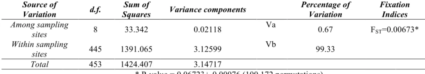
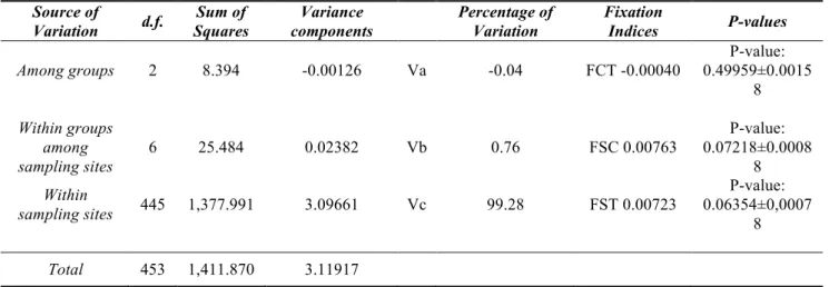
AMOVA
The Analysis of MOlecular VAriance (AMOVA, Excoffier et al., 1992), typically used to test genetic structures and to combine more populations, was used on the global dataset. The AMOVA, in fact, estimate show much of the total variance of
allele frequencies is due to differences between population groups (Va), how much can be attributed to differences between individuals within groups (Vb) and , finally, differences between populations within groups (Vc).
The software Arlequinv.3.1.1 (Excoffier, Laval and Schneider, 2005) estimates the“F” fixation indices from Wright (Wright, 1951, 1965), based on the variance components which measure the loss of heterozygosity compared to HWE or the increase of homozygosity that inevitably leads to 'fix' one or another allele, thus allowing an integrated view of genetic variation and population structure at different hierarchical levels.
The significance level of fixation indices was tested randomly permuting 1,000 times, genotypes, individuals, or populations, between individuals, between populations, or among groups of populations (Excoffier et al., 1992). After each permutation, the F indices are recomputed and compared with the observed one, so it is possible to estimate the frequency with which values equal or exceed the ones in the observed distribution. Then the associated probability that values would be observed by chance is calculated. If these values are significantly greater than zero, i.e., a probability of being observed by chance less than 0,05, they indicate the presence of differentiation. Bayesian analysis in Structure
AMOVA was joined with a further analys is also aimed at verifying the possible presence of underlying genetic structure in the sample. This analysis is based on the method from Pritchard et al. (2000), implemented in the software Structure v.2.3.3, that applies a Bayesian approach to define clusters of individuals based on allele frequencies of multiple loci, without considering population groups defined a priori.