A Comparison of MCMC Sampling for Probabilistic Logic Programming

(1)

Probabilistic Logic Programming

Damiano Azzolini1[0000−0002−7133−2673]_{, Fabrizio Riguzzi}2[0000−0003−1654−9703]_,

Franco Masotti2[0000−0002−1736−3858]_{, and Evelina Lamma}1[0000−0003−2747−4292] 1 _{Dipartimento di Ingegneria – University of Ferrara}

Via Saragat 1, I-44122, Ferrara, Italy

2 _{Dipartimento di Matematica e Informatica – University of Ferrara}

Via Saragat 1, I-44122, Ferrara, Italy

[damiano.azzolini,fabrizio.riguzzi,evelina.lamma]@unife.it, franco.masotti@student.unife.it

Abstract. Markov Chain Monte Carlo (MCMC) methods are a class of algorithms used to perform approximate inference in probabilistic mod-els. When direct sampling from a probability distribution is difficult, MCMC algorithms provide accurate results by constructing a Markov chain that gradually approximates the desired distribution. In this pa-per we describe and compare the pa-performances of two MCMC sampling algorithms, Gibbs sampling and Metropolis Hastings sampling, with re-jection sampling for probabilistic logic programs. In particular, we anal-yse the relation between execution time and number of samples and how fast each algorithm converges.

Keywords: Approximate Inference, Markov Chain Monte Carlo, Probabilistic Logic Programming.

1 Introduction

Probabilistic Logic Programming (PLP) is a useful paradigm for encoding mod-els characterized by complex relations heavily depending on probability [10,13]. One of the main challenges of PLP is to find the probability distribution of query random variables, a task called inference. Real world problems often re-quire very complex models. In this case, exact inference, which tries to compute the probability values in an exact way, is not feasible. Approximate inference overcomes this issue providing approximate results whose accuracy increases as the simulation continues. Markov Chain Monte Carlo methods are a class of algorithms used to perform approximate inference, especially when direct sam-pling from the probability distribution is not practical. In this paper we propose the first Gibbs sampling algorithm for PLP and we analyse how MCMC algo-rithms, Metropolis Hastings sampling and Gibbs sampling in particular, behave in terms of execution time and accuracy of the computed probability.

The paper is structured as follows: in Section 2 we introduce Probabilistic Logic Programming. In Section 3 we offer an overview of Markov Chain Monte

(2)

Carlo (MCMC) techniques and we analyse Metropolis Hastings sampling and Gibbs sampling. Section 4 shows the results of our experiments and Section 5 concludes the paper.

2 Probabilistic Logic Programming

Several approaches have been proposed for combining logic programming and probability theory. Here we consider languages based on the distribution seman-tics proposed by Sato in [15]. All the languages based on this semanseman-tics presented so far differ only in the way they encode choices for clauses but they all have the same expressive power [13].

A probabilistic logic program without function symbols defines a probability distribution over normal logic programs called instances or worlds. Logic Pro-grams with Annotated Disjunctions (LPADs) [16] are a PLP language based on the distribution semantics. In these types of programs, the possible choices are encoded using annotated disjunctive heads of clause. An annotated disjunctive clause has the form h1: Π1; . . . ; hm: Πm: − b1, . . . , bn, where h1, . . . , hmare

log-ical atoms, b1, . . . , bnare logical literals and Π1, . . . , Πmare real numbers in the

interval [0, 1] that sum to 1. b1, . . . , bn is called body while h1: Π1; . . . ; hm: Πm

is called head. In case ofPm

k=1Πm < 1, the head of the annotated disjunctive

clause implicitly contains an extra atom null that does not appear in the body of any clause and whose annotation is 1 −Pm

k=1Πm.

Each world is obtained by selecting one atom from the head of each grounding (i.e. substitution of variables with terms in all possible ways) of each annotated disjunctive clause.

Consider the following LPAD:

mistake(X) : 0.6 : − drunk(X). mistake(X) : 0.7 : − bad player(X). drunk(iverson).

bad player(iverson).

This program can be read as: if X is drunk, then X makes a mistake with probability 0.6 and nothing happens with probability 1 − 0.6 = 0.4. If X is a bad player, then X makes a mistake with probability 0.7 and nothing happens with probability 0.3. The last two clauses state that iverson certainly is a bad player and is drunk.

The probability of a query in a probabilistic logic program without function symbol is computed by extending the probability distribution over normal logic programs defined by the probabilistic logic program, to a joint distribution of the query and the worlds. Then, the probability is obtained by summing out the worlds. When a program contains also function symbols, the previous definition must be extended. This is because its grounding is infinite. So, the number of atomic choices in a selection that defines a world is infinite as well as the number of words. For a detailed definition see [12].

(3)

Performing inference, i.e. computing the probability distribution of the truth values of a query, can be done using exact or approximate methods. Exact in-ference can be performed in a reasonable time only when the size of the domain is relatively small, due to the #P-completeness of the task [7]. For larger do-mains, approximate inference is needed. Moreover, in programs with function symbols, goals may have an infinite number of possible infinite explanations and exact inference may not terminate [13]. Consider a one-dimensional random walk problem where a particle starts at position X > 0. At each time step, the particle can move one unit left (−1) or right (+1) with equal probability. The walk stops as soon as the particle reaches 0. In this case, the walk terminates with probability one [5] but there is an infinite number of walks with nonzero probability [6]. In this example, exact inference, which tries to find the set of all explanations and then computing the probability of the query from it, will loop because the number of explanations is infinite.

Approximate algorithms using sampling are implemented in cplint [14] in the MCINTYRE [11] module. To be able to sample a query from a program, MCINTYRE applies a program transformation to the original program and then queries the modified program. Consider a disjunctive clause

Ci= hi1: Πi1∨ . . . ∨ himi : Πimi : − bi1, . . . , bini,

where Pmi

k=1Πik = 1. Ci is transformed into the set of clauses M C(Ci) =

{M C(Ci, 1), . . . , M C(Ci, mi)}: M C(Ci, 1) = hi1 : − bi1, . . . , bini, sample head(P L, i, V C, N H), N H = 1. . . . M C(Ci, mi) = himi : − bi1, . . . , bini, sample head(P L, i, V C, N H), N H = mi.

where V C is a list containing each variable appearing in Ci and P L is a list

containing [Πi1, . . . , Πimi]. If the parameters do not sum up to 1, the last clause

(the one for null ) is omitted. In other words, a new clause is constructed for each head. Then, using the predicate sample head/4, a head index is sampled at the end of the body. If this index coincides with the head index, the derivation succeeds, otherwise it fails. The internal database of the SWI-Prolog engine [17] is used to record all samples (sampled random choices) taken with sample head/4 using the predicate assertz/1. Notice that sample head/4 is placed at the end of the body because at that point all the variables of the clause are ground (since we assume that the program is range restricted). The truth of a query in a sampled program can be tested by asking the query to the resulting normal program. This is equivalent to taking a sample of the query.

In general we are interested in computing approximate conditional proba-bilities: we want to compute the probability of an event Y = y given that an event E = e has been observed (i.e. P (y | e)) where Y and E are conjunctions of ground atoms and y and e are either true or false. In the rest of the pa-per we analyze three different algorithms available in cplint [14] for pa-performing approximate inference with sampling: Gibbs sampling (Subsec. 3.1), Metropolis-Hastings (Subsec. 3.2) and rejection sampling.

(4)

Rejection sampling [7] is one of the simplest Monte Carlo algorithms. To take a sample of the query, it works in two steps: 1) it queries the evidence e. 2) If the query is successful, it queries the goal g in the same sample (that is, computing P (g | e)). Otherwise it discards the sample. The pseudocode for rejection sampling is shown in Algorithm 1.

Algorithm 1 Function Rejection: Rejection sampling algorithm. 1:function Rejection Sampling(P, query, evidence, Samples)

2: Input: Program P, query, evidence, number of samples Samples

3: Output: P (query|evidence)

4: Succ ← 0

5: n ← 1

6: while n ≤ Samples do

7: Call evidence

8: if evidence succeeds then

9: Call query

10: if query succeeds then

11: Succ ← Succ + 1 12: end if 13: n ← n + 1 14: end if 15: end while 16: return Succ/Samples 17: end function

However, rejection sampling has a disadvantage: if the evidence is very un-likely, many samples are discarded, making the algorithm very slow. For exam-ple, if the probability of the evidence (P (e)) is very low, say 10−4, then even for N = 105 samples the expected number of unrejected samples is 10. So, to obtain at least Samples unrejected samples, we need to generate on average N = Samples/P (e) samples from the distribution [7]. There are several alter-natives to deal with low probability evidence, such as likelihood weighting [3] or Markov Chain Monte Carlo (MCMC) methods.

3 MCMC Sampling

Markov Chain Monte Carlo (MCMC) methods generate samples from the pos-terior distribution when directly sampling from the pospos-terior is not feasible, due to the complexity of the distribution itself. The main idea of MCMC methods is to iteratively construct a Markov chain in which sampling can be done directly. As the number of samples increases, the approximation gets closer to the desired posterior distribution. In this way, MCMC methods are theoretically capable of getting arbitrarily close to the true posterior distribution. During the execution of MCMC algorithms, usually the first few samples are discarded because they may not represent the desired distribution. This phase is called burnin phase.

In this section we analyse two of the most famous MCMC sampling algo-rithms: Gibbs sampling and Metropolis Hastings sampling.

(5)

Algorithm 2 Function Gibbs: Gibbs MCMC algorithm 1:function Gibbs(query, evidence, M ixing, Samples, block)

2: GibbsCycle(query, evidence, M ixing, block)

3: return GibbsCycle(query, evidence, Samples, block)

4:end function

5:function GibbsCycle(query, evidence, Samples, block)

6: Succ ← 0

7: for n ← 1 → Samples do

8: Save a copy of samples C

9: SampleCycle(evidence)

10: Delete the copy of samples C

11: ListOfRemovedSamples = RemoveSamples(block)

12: Call query . new samples are asserted at the bottom of the list

14: Succ ← Succ + 1 15: end if 16: CheckSamples(ListOfRemovedSamples) 17: end for 18: return Succ Samples 19: end function 20: procedure SampleCycle(evidence) 21: while true do 22: Call evidence

24: T rueEv ← true

25: return

26: end if

27: Erase all samples

28: Restore samples copy C

29: end while

30: end procedure

31: function RemoveSamples(block)

32: SampleList ← []

33: for b ← 1 → block do

34: retract sample S = (Rule, Substitution, V alue) . samples are retracted from the top of the list

35: Add (Rule, Substitution) to SampleList

36: end for

37: return SampleList

38: end function

39: procedure CheckSamples(ListOfRemovedSamples)

40: for all (Rule, Substitution) ∈ ListOfRemovedSamples do

41: if (Rule, Substitution) was not sampled then

42: Sample a value for (Rule, Substitution) and record it with assert

43: end if

44: end for

45: end procedure

3.1 Gibbs Sampling

The idea behind Gibbs sampling is the following: when sampling from a joint distribution is not feasible, we can sample each variable independently consid-ering the other variables as observed [4]. In details, suppose we have n variables X1, . . . , Xn. First we set these variables to an initial value x

(0) 1 , . . . , x

(0) n , for

instance by sampling from a prior distribution. At each iteration (or until con-vergence) we take a sample x(t)m ∼ P (xm| xt−11 , x

t−1 2 , . . . , x t−1 m−1, x t−1 m+1, . . . , xt−1n ).

(6)

to-gether two or more variables and sampling from their joint distribution condi-tioned on all other variables, instead of sampling each one individually.

Gibbs sampling is available on cplint. The code is shown in Algorithm 2. A list of sampled random choices is stored in memory using Prolog asserts. Function GibbsCycle performs the main loop. To take a sample, we query the evidence using function SampleCycle that performs a type of rejection sampling: it queries the evidence until the value true is obtained. When the evidence succeeds, we remove block random choices from the list of saved random choices using function RemoveSamples. Then, we ask the query and, if the query is successful, the number of successes is incremented by 1. The last step consist in calling function CheckSamples. This function checks if there are some rules not sampled in the list of removed random choices. If so, a value is sampled and stored in memory. This is due to the necessity of assigning a value to xm even if it was not involved in the new derivation of the query. The

probability is returned as the ratio between the number of successes and the total number of samples.

3.2 Metropolis Hastings

In Metropolis Hastings sampling, a Markov chain is built by taking an initial sample and, starting from this sample, by generating successors samples. Here we consider the algorithm developed in [9] and implemented in cplint [14]. Al-gorithm 3 goes as follows: 1) it samples random choices so that the evidence is true to build an initial sample. 2) It removes a fixed number (defined as lag) of sampled probabilistic choices to build the successor sample. 3) It queries again the evidence by sampling starting from the undeleted samples. 4) If the evi-dence succeeds, the query is asked by sampling. It is accepted with probability min{1, N0/N1} where N0is the number of choices sampled in the previous

sam-ple and N1 is the number of choices sampled in the current sample. 5) If the

query succeeds in the last accepted sample then the number of successes of the query is increased by 1. 6) The final probability is computed as the number of successes over the total number of samples.

In details, function MH returns the probability of the query given the ev-idence. Function resample(lag) deletes lag choices from the sampled random choices. In [9] lag is always 1. Function InitialSample builds the initial sample with a meta-interpreter that starts with the goal and randomizes the order in which clauses are used for resolution during the search to make the initial sample unbiased. This is achieved by collecting all the clauses that match a subgoal and trying them in random order. Then the goal is queried using regular sampling.

4 Experiments

We tested the performances of Gibbs sampling, Metropolis Hastings sampling, and rejection sampling using four different programs. For each program, we ran the queries mc gibbs sample/5, mc mh sample/5 and mc rejection sample/5

(7)

Algorithm 3 Function MH: Metropolis-Hastings MCMC algorithm 1:function MH(query, evidence, lag, Samples)

2: MHCycle(query, evidence, lag)

3: return MHCycle(query, evidence, Samples)

4:end function

5:function MHCycle(query, evidence, Samples)

6: T rueSamples ← 0

7: Ssample ← InitialSample(evidence)

8: Call query

10: querySample ← true

11: else

12: querySample ← f alse

13: end if

14: Save a copy of the current samples C

15: n ← 0

16: while n < Samples do

17: n ← n + 1

18: SamplesList ← Resample(lag)

19: Call evidence

21: Call query

23: querySample0← true

24: else

25: querySample0← f alse

26: end if

27: let CurrentSampled be the current number of choices sampled

28: if min(1,_{P reviousSampled}CurrentSampled) > RandomV alue(0, 1) then

29: P reviousSampled ← CurrentSampled

30: Delete the copy of the previous samples C

31: Save a copy of the current samples C

32: querySample ← querySample0

33: else

36: end if

37: else

40: end if

41: end while

43: Delete the copy of the previous samples C

44: returnT rueSamples_Samples

45: end function

46: function Resample(lag)

47: for n ← 1 → lag do

48: Delete a sample Sample

49: N ewSample ← Sample(Ssample)

50: Assert N ewSample

51: end for

52: return SamplesList

53: end function

provided by the MCINTYRE module [11] implemented in cplint. All the algo-rithms are written in Prolog and tested in SWI-Prolog [17] version 8.1.7. For each query we show how the number of samples affects the execution time and the computed probability. All the experiments were conducted on a cluster3

with Intel R _Xeon R _{E5-2630v3 running at 2.40 GHz. Execution times are} com-3

(8)

puted using the SWI-Prolog built-in predicate statistics/2 with the keyword walltime. The results are averages of 10 runs. For both Gibbs and Metropolis Hastings sampling, we set the number of deleted samples (burnin) to 100.

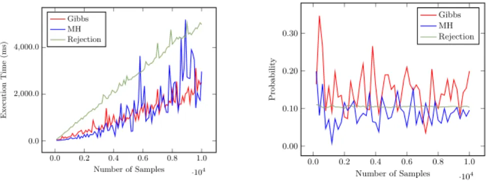
For the first comparison, we consider a program that generatively defines a random arithmetic function4_{. The problem is to predict the value returned by the}

function given one or two couples of input-output, i.e., to compute a conditional probability. The peculiarity of this program is that it has an infinite number of explanations. As described in Section 2, approximate inference is needed, as exact inference may loop. In this example, the evidence has probability 0.05. Results are shown in Fig. 1. In this case, Metropolis Hastings sampling and Gibbs sampling have comparable execution time, but Gibbs sampling converges more slowly. 0.0 0.2 0.4 0.6 0.8 1.0 ·104 0.0 2,000.0 4,000.0 Number of Samples Execution Time (ms) Gibbs MH Rejection 0.0 0.2 0.4 0.6 0.8 1.0 ·104 0.00 0.10 0.20 0.30 Number of Samples Probabilit y Gibbs MH Rejection

Fig. 1. Results for random arithmetic functions test.

The second program encodes a hidden Markov model (HMM) for modeling DNA sequences. The model has three states, q1, q2 and end, and four output symbols, a, c, g, and t, corresponding to the four nucleotides (letters)5 _{[2]. We}

compute the probability that the model emits the sequence [a,c] observing that from state q1 the models emits the letter a. The evidence has probability 0.25. Results are shown in Fig. 2. In this case, all the three algorithms converge to the same probability value, but Metropolis Hastings is the slowest one with execution time several times larger than Gibbs and rejection sampling.

For the third test we consider a Latent Dirichlet Allocation (LDA) model6[1]. LDA is a generative probabilistic model especially useful in text analysis. In particular, it models the distribution of terms and topics in documents in order to predict the topic of the analysed text. This program, differently from the others, is hybrid, i.e., it contains also continuous random variables. For this

4 _{http://cplint.eu/example/inference/arithm.pl} 5

http://cplint.eu/example/inference/hmm.pl

6

(9)

0.0 0.2 0.4 0.6 0.8 1.0 ·104 0.0 2,000.0 4,000.0 6,000.0 8,000.0 Number of Samples Execution Time (ms) Gibbs MH Rejection 0.0 0.2 0.4 0.6 0.8 1.0 ·104 1.0 1.5 2.0 2.5 ·10−2 Number of Samples Probabilit y Gibbs MH Rejection

Fig. 2. Results for HMM test.

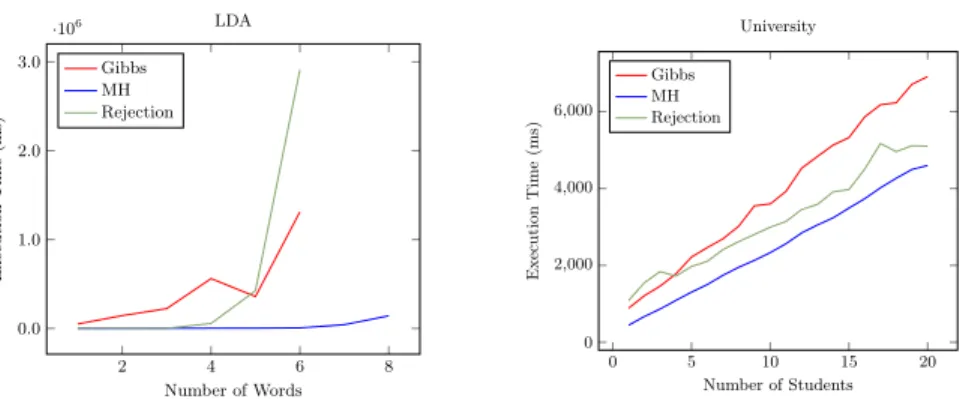
test, we fix both the number of words considered in a document (10) and the number of topics (2) and we compute the relation between number of samples, probability and execution time. In this example, we observe that the first two words of the document are equal, which has probability 0.01. The results are shown in Fig.3: in this case Gibbs sampling is slower than Metropolis Hastings both in execution time and number of samples needed to compute an accurate probability. Then we also fix the number of topics to 2 and increase the number of consecutive equal words from 1 to 8. In this test, the evidence is progressively extended, i.e., we observe that n number of words (from 1 to 8) are equal. In this case Metropolis Hastings sampling outperforms the other algorithms (Fig. 4 left). For Gibbs sampling and rejection sampling, the number of words in the plot is at most 6 since, for a value bigger than that, each query requires more than one hour of computation.

The last program describes a university domain7 [8] characterized by stu-dents, professors and courses. Each professor is related to a course and each student attends a course. We are interested in computing the probability that a professor teaches a course given that the same professor is advisor of some stu-dents of the same course. We fixed the number of stustu-dents to 10, and both the number of professors and courses to 1. In this case the evidence has probability 0.09. Results are shown in Fig. 5. As for the previous experiment, we also incre-mented the number of students up to 20 and plot how execution time changes (Fig. 4 right). In both cases, Gibbs sampling is still the slowest algorithm, but the performances are not so different from Metropolis Hastings and rejection sampling.

7

(10)

0 1,000 2,000 3,000 4,000 0.0 1.0 2.0 ·104 Number of Samples Execution Time (ms) Gibbs MH Rejection 0.0 1,000.0 2,000.0 3,000.0 4,000.0 0.2 0.4 0.6 0.8 Number of Samples Probabilit y Gibbs MH Rejection

Fig. 3. Results for LDA model.

2 4 6 8 0.0 1.0 2.0 3.0 ·106 Number of Words Execution Time (ms) LDA Gibbs MH Rejection 0 5 10 15 20 0 2,000 4,000 6,000 Number of Students Execution T ime (ms) University Gibbs MH Rejection

Fig. 4. Both graphs show how the number of facts affects the execution time. The left one is related to the LDA model while the right one to the university model. For both we fixed the number of samples to 104_.

5 Conclusions

In this paper we proposed the first Gibbs sampling algorithm for PLP. We also compared it with Metropolis-Hastings and rejection sampling. The three algo-rithms are available in the cplint suite and online in the web applicationcplint.eu. For each algorithm we conducted several experiments to compare execution time and convergence time. In three of the four experiments, Metropolis Hastings outperformed Gibbs sampling and rejection sampling in terms of accuracy and execution time. However, in the second experiment (HMM), Gibbs sampling has better performances than Metropolis Hastings and it is comparable to rejection sampling in terms of execution time. Also, in this test, Metropolis Hastings is the least accurate (it overestimates the probability) while Gibbs sampling and

(11)

0 0.2 0.4 0.6 0.8 1 ·104 0 1,000 2,000 3,000 4,000 Number of Samples Execution Time (ms) Gibbs MH Rejection 0 2,000 4,000 6,000 8,000 0.1 0.1 0.2 0.2 Number of Samples Probabilit y Gibbs MH Rejection

Fig. 5. Results for the university domain.

rejection sampling converge faster. Experimental analysis showed that Metropo-lis Hastings is the fastest among the three unless the evidence has a relatively high probability as in HMM where it has probability 0.25: in that case, Gibbs performs better.

References

1. Blei, D.M., Ng, A.Y., Jordan, M.I.: Latent Dirichlet allocation. J. Mach. Learn. Res. 3, 993–1022 (2003)

2. Christiansen, H., Gallagher, J.P.: Non-discriminating arguments and their uses. In: Logic Programming, 25th International Conference, ICLP 2009, Pasadena, CA, USA, July 14-17, 2009. Proceedings. Lecture Notes in Computer Science, vol. 5649, pp. 55–69. Springer (2009)

3. Fung, R.M., Chang, K.C.: Weighing and integrating evidence for stochastic simu-lation in bayesian networks. In: 5th Conference Conference on Uncertainty in Ar-tificial Intelligence (UAI 1989). pp. 209–220. North-Holland Publishing Co. (1989) 4. Geman, S., Geman, D.: Stochastic relaxation, gibbs distributions, and the bayesian restoration of images. In: Readings in computer vision, pp. 564–584. Elsevier (1987) 5. Hurd, J.: A formal approach to probabilistic termination. In: Carre˜no, V., Mu˜noz, C.A., Tahar, S. (eds.) TPHOLs 2002. LNCS, vol. 2410, pp. 230–245. Springer (2002). https://doi.org/10.1007/3-540-45685-616

6. Kaminski, B.L., Katoen, J.P., Matheja, C., Olmedo, F.: Weakest precondi-tion reasoning for expected run-times of probabilistic programs. In: Thie-mann, P. (ed.) ESOP 2016. LNCS, vol. 9632, pp. 364–389. Springer (2016). https://doi.org/10.1007/978-3-662-49498-115

7. Koller, D., Friedman, N.: Probabilistic Graphical Models: Principles and Tech-niques. Adaptive computation and machine learning, MIT Press, Cambridge, MA (2009)

8. Meert, W., Struyf, J., Blockeel, H.: Learning ground CP-Logic theories by lever-aging Bayesian network learning techniques. Fund. Inform. 89(1), 131–160 (2008) 9. Nampally, A., Ramakrishnan, C.: Adaptive MCMC-based inference in probabilistic

(12)

10. Nguembang Fadja, A., Riguzzi, F.: Probabilistic logic programming in action. In: Holzinger, A., Goebel, R., Ferri, M., Palade, V. (eds.) Towards Integrative Ma-chine Learning and Knowledge Extraction, LNCS, vol. 10344. Springer (2017). https://doi.org/10.1007/978-3-319-69775-8 5

11. Riguzzi, F.: MCINTYRE: A Monte Carlo system for probabilistic logic program-ming. Fund. Inform. 124(4), 521–541 (2013). https://doi.org/10.3233/FI-2013-847 12. Riguzzi, F.: The distribution semantics for normal programs with function symbols. Int. J. Approx. Reason. 77, 1–19 (2016). https://doi.org/10.1016/j.ijar.2016.05.005 13. Riguzzi, F.: Foundations of Probabilistic Logic Programming. River Publishers,

Gistrup, Denmark (2018)

14. Riguzzi, F., Bellodi, E., Lamma, E., Zese, R., Cota, G.: Probabilistic logic programming on the web. Softw.-Pract. Exper. 46(10), 1381–1396 (10 2016). https://doi.org/10.1002/spe.2386

15. Sato, T.: A statistical learning method for logic programs with distribution seman-tics. In: Sterling, L. (ed.) ICLP 1995. pp. 715–729. MIT Press (1995)

16. Vennekens, J., Verbaeten, S., Bruynooghe, M.: Logic programs with annotated disjunctions. In: Demoen, B., Lifschitz, V. (eds.) ICLP 2004. LNCS, vol. 3131, pp. 431–445. Springer (2004). https://doi.org/10.1007/978-3-540-27775-030

17. Wielemaker, J., Schrijvers, T., Triska, M., Lager, T.: SWI-Prolog. Theor. Pract. Log. Prog. 12(1-2), 67–96 (2012). https://doi.org/10.1017/S1471068411000494