Stochastic optimization for airport inventory management

(1)

UNIVERSITÀ DEGLI STUDI

ROMA

TRE

Roma Tre University

Ph.D. in Computer Science and Automation

Stochastic optimization for

airport inventory management

(2)

(3)

Stochastic optimization for airport inventory management

A thesis presented by Annalisa Cesaro

in partial fulfillment of the requirements for the degree of Doctor of Philosophy

in Computer Science and Automation Roma Tre University

Dept. of Computer Science and Automation 30 March 2010

(4)

Committee:

Prof. Dario Pacciarelli

Reviewers:

Prof. A. Agnetis

(5)

(6)

(7)

Acknowledgments

Con la conclusione di questa tesi, si chiude un periodo intenso della mia vita, in cui le esperienze vissute sono state molteplici e variegate.

Il percorso dottorale `e un percorso ricco di libere opportunit`a.

Ringrazio chi mi ha permesso di iniziare questo percorso, il mio tutor Dario Pacciarelli, che `e sempre stato un costruttivo punto di riferimento in tutti questi anni e che mi ha dato tanto.

Ringrazio Gianluca, per il suo amore e sostegno sempre.

Ringrazio i miei 4 angeli custodi: i miei genitori ed i genitori di Gianluca, senza di loro non sarei potuta venire serenamente a lavorare all’universit`a, sapendo di avere affidato mio figlio in mani premurose e sicure.

Ringrazio anche te, Vittorio: anche se cos`ı piccolo, doni gioia, grinta e forza. Vi amo tesori miei.

Ringrazio gli altri dottorandi del laboratorio e del dipartimento, sia chi an-cora qui e sia chi lontano, con cui abbiamo condiviso esperienze e momenti di soddisfazione o sconforto.

Ringrazio tutte le persone che ho incontrato nelle varie scuole o conferenze, perch`e ognuna sapeva comunicare la propria passione nel raggiungere un tra-guardo.

(8)

List of Tables

3.1 Two non solvable instances. . . 54

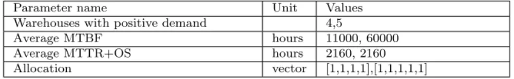
3.2 Parameter values for the computational experiment . . . 56

3.3 Numerical results . . . 56

4.1 Five non solvable instances. . . 76

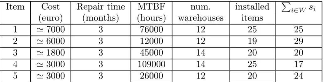
5.1 Parameter values for the computational experiment . . . 95

5.2 Performance of ISA and BB algorithms for the 12 items . . . 96

5.3 Performance of ISA and BB for different holding costs . . . 97

(11)

List of Figures

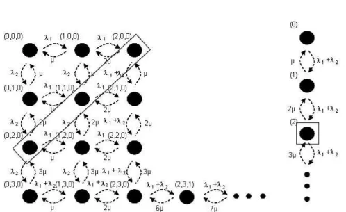
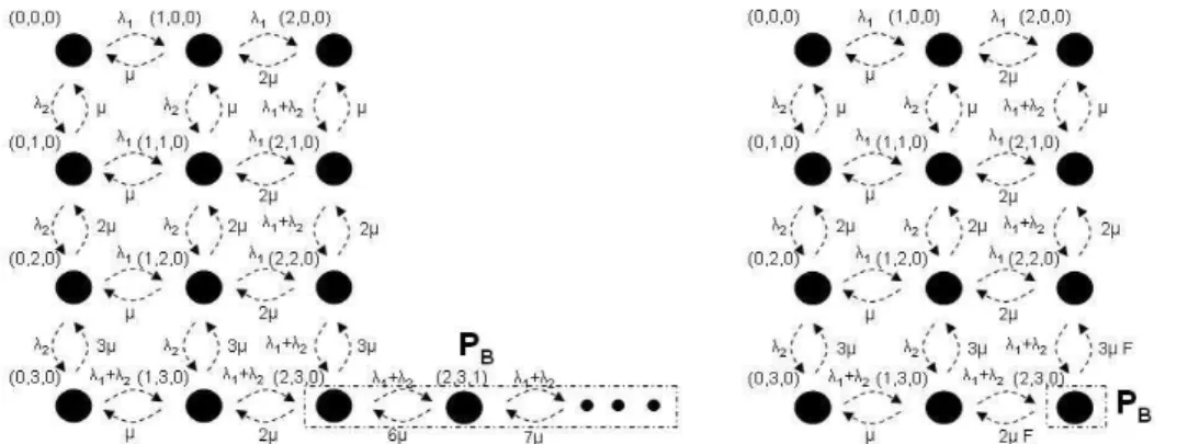
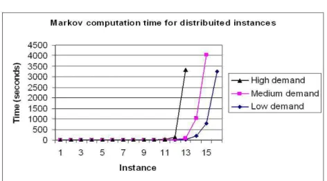
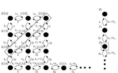
1.1 Logistics chain system: two echelon (left) and single echelon (right) 3 3.1 A Markov chain (left) and the aggregated birth death model (right) 43 3.2 A Markov chain with infinite (left) and finite (right) number of states. 45 3.3 Computation time for the Markov chain model and distributed

in-stances. . . 53

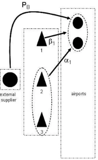
3.4 Memory effort for the Markov chain model and distributed instances. 53 4.1 A Markov chain (left) and the aggregated birth death model (right) 65 4.2 The three fractions α1, β1 and PB(S) of demand at warehouse 1. . 67

4.3 Equivalent system . . . 69

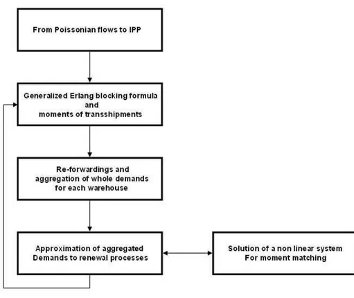
4.4 Iterative procedure for estimating steady state IPP parameters . . 73

4.5 Computation time for the Markov chain model and distributed in-stances. . . 76

4.6 Memory effort for the Markov chain model and distributed instances. 77 4.7 Computation time for the approximate models and practical instances. 78 4.8 Memory effort for the approximate models and practical instances. 78 4.9 Computation time (left) and memory effort (right) for the approx-imate models and random instances. . . 79

4.10 Percentage error for practical instances . . . 80

4.11 Percentage error for random instances . . . 81

4.12 4 sample instances: OA varying for different scale factor values . . 81

5.1 Pseudocode of the heuristic for Initial Spares Allocation . . . 92

5.2 Pseudocode of the BB algorithm . . . 94

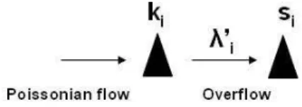
A.1 Sketch of IPP process . . . 127

A.2 Sketch of IPP overflow process . . . 128 xi

(12)

xii List of Figures

A.3 Pseudocode of the algorithm for the trust region approach . . . 148 A.4 Pseudocode of the algorithm for the cauchy point approximation . 152 A.5 Pseudocode of the algorithm for the trust region approach . . . 156

(13)

Chapter 1 Introduction

1.1. Airport inventory management

The ever increasing air traffic demand of passengers and cargos all over the world is currently limited by the capacity of the airports, which are expected to become a serious bottleneck for air traffic in a near future [1]. Facing such growth requires significant investments for developing existing airports and/or constructing new ones. Specifically, there is an increasing need for safety equipments in order to grant airport safety, as well as for supporting the correct execution of airport operations. In this scenario airports face every day the challenging task of maintaining high standards of safety at a sustain-able cost. In such a context maintenance plays an important role. Preventive maintenance is scheduled in advance and anticipates the realization of equip-ment failures. Corrective maintenance is carried out upon a failure happens in a system. Typically, when a failure of some equipment takes place, failed components must be promptly replenished with new spare parts, since safety standards are not compatible with long repairing times. As observed by sev-eral authors, see e.g. by [43], the logistics of spare parts differs from those of other materials in several ways. Equipments may have remarkable costs, long repairing times and sporadic failures. The latter are difficult to forecast and cause relevant financial effects, due to the economical and legal implications of a lack of safety of airport operations. These characteristics are particu-larly stringent in the airport context, where therefore maintenance deserves substantial attention. Maintenance concerns aftermarket service, which im-portance today is in general high. Deloitte [26] discusses of service revolution,

(14)

2 CHAPTER 1. INTRODUCTION

because the high combined revenues due to aftermarket service in Aerospace, Defence, Automotive and High Tech. Specifically, it reports that in Aerospace and Defence on average service revenues account for 47% of the total business and that profitability is much higher that in the primary product business. It follows clearly that improving aftermarket processes and resource allocation is crucial in aerospace business. The sporadic nature of the failure process for a single equipment translates in most cases into very low demand for spare parts. For an item there are typically less than ten working equipments with MTBF equal to six years or more. Therefore, for economical reasons, airports are usually grouped on a regional base and served by a single warehouse. For example, the Italian territory is divided in 17 service regions serving a total of 38 civil airports [30]. Each spare part warehouse manages the aggregated demand of all the airports encompassed in its region. It follows that the ag-gregated demand rate for some items may be low or high, depending on the number of working equipments in the area. The spare parts supply chain may typically involve at least three actors: airport authorities, logistics companies and equipment suppliers. The latter are responsible for supplying new compo-nents and/or repaired items, which usually require long replenishment times. Intermediate logistic companies are in charge of replenishing spare parts in the short term, by granting minimum levels of operational availability (i.e., the fraction of time during which all working equipments are operative) regu-lated by contracts with airport authorities. Clearly the best design of resupply networks and the optimal allocation of inventories within these networks is of unquestionable importance to the economical maintenance of equipment. The types of decisions that must be made relating to service parts can roughly be divided into three planning categories: strategic planning, tactical planning and operational planning. Strategic planning is an on-going activity that has two primary functions. First, the definition of customer requirements, e.g. the range of service parts needed and timeliness of these needs, today and for the next several years. Second, the definition of the resources to meet customer requirements, e.g. the operating environment, the information systems, the supply chain partners. From the perspective of service parts, tactical planning establishes what inventories will be required to meet operational objectives at some future time, given the design and the operational characteristics of an ex-istent resupply system infrastructure. Finally, the third category of planning concern operational decisions, which are based on real-time execution prob-lems, are formulated over short planning horizons and contain more details on current operating limitations.

(15)

1.2. RESEARCH MOTIVATION 3

1.2. Research motivation

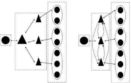
This thesis is devoted to constructing mathematical models that can be ef-fectively used to carry out the tactical planning goal of determining systems stock levels. Our case study is motivated by the practical needs of an Italian logistics company supporting the activity of 38 civil airports spread over the Italian territory. The company handles 17 warehouses and manages the overall processes of purchasing, holding, ensuring that the overall reliability of safety equipments is always within contractual limits. The aim of the company is therefore to grant the prescribed quality of service at minimum cost. To this aim, a two echelon inventory policy without lateral transshipments is currently adopted and the level of stock and geographical allocation of spare parts is obtained with the VARIMETRIC algorithm of [74]. This policy is depicted in figure 1(left).

Figure 1.1: Logistics chain system: two echelon (left) and single echelon (right)

Effective supply chain management is currently recognized as a key deter-minant of competitiveness and success in manufacturing and services, because the implementation of supply chain management has significant impact on cost service and quality. Numerous strategies for achieving these targets have been proposed. One such strategy allows movements of stock between locations at the same echelon level or across different levels. These stock movements are

(16)

termed lateral transshipments, or simply transshipments. As a demand oc-curs under the implementation of transshipment strategy, there will be three possible activities: the demand is met from the stock on hand or it is met via transshipment from another location or it is backordered. In other words, firstly, if a location’s on hand inventory level is greater than the demand size, than the demand is met. Secondly, if the on-hand inventory is positive but less than the demand size, than it is used to partially satisfy the demand and the remaining demand is met either via transshipment or is backordered. Thirdly, if the on-hand inventory level is zero, the demand is met via transshipment or is backordered under the assumption of no lost sales. Therefore, trans-shipment policy can improve stock availability, customer service level. without increasing stock level which may induce higher inventory relevant cost. In other words, transshipments enable the sharing of stock among locations, they facil-itate each location as a secondary, random supply source for the remainder. If transshipment is not limited to one direction, the locations which meet their demand via transshipment form a pool. Thus, the locations’ replenishment can be coordinated and even combined in order to avoid excessive inventory costs. The improvements in information technology coupled with the substan-tial reduction in the cost of processing, storing and analyzing data have made sharing of inventories more attractive. Furthermore, logistics companies, such as UPS, have made the rapid movement of parts from one place to another possible and more affordable. The underlying question that must be addressed is: which is the impact of lateral resupply on inventory levels and operations. A number of authors have addressed this issue. Several simulation studies have demonstrated the effects of lateral resupply in multi-echelon systems [32], [33], [73]. While the environments that were analyzed by these authors did differ, their results showed that in a wide variety of circumstances, lateral resupply among locations is a very effective way to improve customer service and lower inventory investments. Other authors have presented and tested many analytic models that explicitly consider the possibility of supplying location through lat-eral transshipments. For example, see Archibald [3], Lee [59], Alfredsson and Verrijdt [2], Axsater [4], Taragas [79], [81], Taragas and Cohen [80], Sherbrooke [73]. These models differ in many ways. Some are stationary, continuous time models, while other are periodic review. Essentially, though, all these analytic models are tactical planning models. They are either economic models that suggest what quantities of material to buy or they are models used to deter-mine the probabilities for various events occurring. We say that these models are tactical models because they do not consider the possibility of using all state-of-the-world information when representing the operational environment.

(17)

1.3. RESEARCH OBJECTIVES 5

For example FIFO inventory allocation rules are often assumed as the basis for shipping parts from a central location (depot) to field stocking location. Real time execution systems would take more information into account. Moreover, as observed, e.g., by [54], single echelon models with complete pooling might be more effective for reducing both reaction time to stockouts and inventory levels. In Figure 1(right) a single echelon policy is depicted. At the time of writing, lateral communication is only used by the company in emergency situations, when couriers or overnight carriers rapidly transfer parts to demand locations. However, lateral transshipment is not explicitly included in the model when deciding the spares allocation among the 17 warehouses. Therefore, the com-pany managers are interested in evaluating the potential benefits deriving from the adoption of a single echelon with a complete pooling policy. To this aim, however, there is a need of effective models for assessing the performance of a single echelon replenishment policy. This is not an easy task for large instances even for steady state analysis, as the size of the instance increases, as in case of high rate demand. And finally there is the need of efficient and effective models for allocating optimally the stock in such a context. In fact, in models where lateral transshipment is taken into account, the resulting optimization problems have non-linear constraints (on service levels) and objective and in-teger decision variables (like base stock levels). Especially for problem with large numbers of locations optimization is rough. In such models only explicit enumeration [50] has been proposed for solving the Spares Allocation Problem exactly or many heuristics algorithm have been evaluated in [93], [59], [54], [4] [70].

1.3. Research objectives

Based on the needs summarized above, the following research objectives are the subject of this dissertation. We focus on a single echelon one-for-one ordering policy with complete pooling, with a deterministic rule for lateral transship-ments.

• The main objective is to formalize mathematically the Spares Allocation Problem (SAP) and understand its mathematical structure for building an exact algorithm for optimally allocating the spares. In fact, in litera-ture to the best of our knowledge no exact algorithm has been proposed for allocating optimally the spares in a continuous review setting rather than a total enumerative algorithm. By exploiting the above algorithm it is interesting

(18)

– Making insight in the SAP and underline which factors influence inventories in such a context.

– Evaluating fast and accurate heuristics for SAP.

• Efficient and accurate models for assessing the performance of a single echelon replenishment policy are needed especially for large numbers of locations. A drawback of the policy of interest is the state dependent nature of re-forwardings in the systems, it’s therefore interesting.

– understanding the properties of the Markov chain associated to the chosen policy.

– exploring, despite its state dependent nature, the possibility of ex-pressing the state probabilities of the associated Markov chain model exactly in product form

– developing fast and accurate approximate models for evaluating the performance and costs in the system, since computing the state probabilities is not practical as the number of states in the Markov chain increases.

The achievement of the first objective clearly requires a strong connection with the resolution of the second objective. In fact, the development of an exact algorithm for allocating the spares may require in contexts with a large number of warehouses and high rates approximate models for assessing the performance and evaluating the costs.

1.4. Research contribution

This thesis presents an innovative contribution to the combined resolution of the research objectives of Section 1.3. Next, we briefly introduce the main achievements. We focus on a single echelon one-for-one ordering policy with complete pooling, with a deterministic rule for lateral transshipments. This policy may be modeled through a Markov chain. In fact, a Markov process allows us to model the uncertainty in many real-world systems that evolve dynamically in time. The basic concepts of a Markov process are those of a state and of a state transition. In specific applications the modeling art is to find an adequate state description such that the associated stochastic process indeed has the Markovian property that the knowledge of the present state is sufficient to predict the future stochastic behavior of the process. A Markov chain is a random sequence in which the dependency of the successive events goes back

(19)

1.4. RESEARCH CONTRIBUTION 7

only one unit in time. In other words, the future probabilistic behavior of the process depends only on the present state of the process and is not influenced by its past history. The main interest is the long-run behavior of the Markov chain, i.e. long-run averages are usually required in the analysis of practical applications, to this aim it’ s necessary defining the equilibrium distribution, if any, and computing this distribution, e.g. {πj, j ∈ I}. I is the state space

of the stochastic process. Hence, the equilibrium state probabilities πj may be

determined up to a multiplicative constant by the equilibrium equations πj=

X

k∈I

πk kj

where j ∈ I and pij are the one step state probabilities, when the Markov chain

is assumed time-homogeneous. The multiplicative constant is determined by the normalizing equation

X

j∈I

πh= 1

It’s known that in case of finite state Markov chain in general there are two methods to solve the Markov chain equations: direct and iterative methods, such as the Gauss-Jordan method and the Gauss-Seidel method respectively. What one usually does to solve numerically the infinite set of equilibrium equa-tions is to approximate the infinite-state Markov model by a truncated model with finitely many states so that the probability mass of the deleted states is very small. Indeed, for a finite-state truncation with a sufficiently large num-ber of states, the difference between the two models will be negligible from a computational point of view. However, such a truncation often leads to a finite but very large system of linear equations whose numerical solution will be quite time-consuming, although an arsenal of good methods is available to solve the equilibrium equations of a finite Markov chain. Moreover, it is somewhat dis-concerting that we need a brute-force approximation to solve the infinite-state model numerically. Fortunately, many applications allow for a much simpler and more satisfactory approach to solving the infinite set of state equations. Under rather general conditions the state probabilities exhibit a geometric tail behavior that can be exploited to reduce the infinite system of state equations to a finite set of linear equations. The geometric tail approach results in a finite system of linear equations whose size is usually much smaller than the size of the finite system obtained from a brute-force truncation. Hence, it’s clear that computing the state probabilities is not practical as the number of states in the Markov chain increases In fact, the above methods suffer from computer

(20)

memory problems and for long computation time.

Hence, we have explored the possibility to express the state probabilities of the associated Markov chain model in product form, thus reducing the com-putational effort. We have tested it numerically, but as expected the state dependent nature of re-forwarding in the systems does not allow to express these state probabilities in product form.

Therefore, we adapt four approximation techniques to our model and evalu-ate their performance in terms of computational effort, memory requirement and error with respect to the exact value (objective 2). Three techniques ap-proximate state probabilities with others that can be expressed in product form, so that the Markov chain can be decomposed. Specifically, we adapt a method by Alfredsson and Verrijdt, the Equivalent Random Traffic method and the Interrupted Poisson Process method. The fourth technique is based on the multi-dimensional scaling down approach, which studies an equivalent reduced Markov chain rather than decomposing the original one. The first three methods are based on decomposition approach. State probabilities are approximated with others that can be expressed in product form, so that the Markov chain can be decomposed and operational availability can be easily computed. Specifically, our first method, referred to in the following as the AV method, is a slight modification of a method by Alfredsson and Verrijdt [2]. The second and third method is based on ideas successfully used in the field of telecommunications, and specifically in the Equivalent Random Traffic method (ERT method) [45] and the Interrupted Poisson Process method (IPP method) [56],[61]. With the IPP and ERT methods part of the traffic may be lost when no server is available. In our adaptation of these methods we include the presence of an external supplier to avoid lost requests. The fourth method is based on the multi-dimensional scaling down approach, which studies an equivalent reduced Markov chain rather than decomposing the original one. A scaling down approach is used by Axsater [6] to study a two-echelon policy. We adapt this method to study the single echelon policy with complete pooling in a Markovian framework without decomposing the original chain. Computational experiments, carried on practical data from an airport equipment maintenance context show the accuracy degree and the computational effort required by each approximate method.

A major contribution of this thesis to solving efficiently and timely the Spares Allocation Problem consists in a branch and bound algorithm (objective 1). In literature an exact efficient method to solve SAP in a continuous review setting seems to lack. As noted in [50] it is very likely that no polynomial time optimization algorithm exists for our type of problem. The problem under

(21)

con-1.5. OUTLINE OF THE THESIS 9

sideration in this dissertation could also be considered as a nonlinear knapsack problem. For a general description of knapsack problems, see e.g.[46]. Kellerer et al. [46] prove that even the simplest type of knapsack problem belongs to the class of NP-hard problems. This is generally considered as strong theoret-ical evidence that no polynomial time algorithm exists for computing optimal solutions and thus a good reason for looking for efficient exact enumerative techniques or to apply approximation algorithms. Therefore, after modeling the stock allocation problem as a non convex integer program, we exploit the special structure of the problem to design an efficient branch and bound pro-cedure. Our bounds are obtained by solving a reduced problem with convex objective function, solvable at optimality very efficiently. Computational ex-periments, carried on practical data from an airport equipment maintenance context show that this method efficiently solves at optimality many practical instances.

Different cost scenario are evaluated for understanding which factors influence inventories and when the proposed procedure is more efficient.

Moreover a simple and fast heuristic is computed by distributing spare parts among warehouses with positive demand and by giving preference to ware-houses with larger demand (objective 1). In fact, simulation experiments car-ried out in [15] show that avoiding concentration of spares in few warehouses is an effective allocation policy. The accuracy of such an heuristic is evaluated by comparing it with the branch and bound allocations.

1.5. Outline of the thesis

This section gives a short introduction to each chapter.

Chapter 2 provides an overview of the state-of-knowledge in spare parts pro-visioning. In a first part, some relevant contributions to spare parts inventory control are described. In a second part, we focus on transshipment problems in Supply Chain Systems. Finally we give an overview of some relevant analytical and computational methods, used in the analysis of stock allocation problems where base stock policy is assumed. In fact, because of this assumption we can separate evaluation of a given policy and optimization, the latter giving a value to the decision variables of interest. Therefore, specific methods must be used for evaluation and optimization respectively. Note that the stochastic nature of the problem of interest is taken into account in the analysis of a given policy.

(22)

Chapter 3 introduces the main notation used in this dissertation and the two main mathematical models involved in the SAP analysis and solution. The first is a Markov chain model useful for evaluating the costs and waiting times in the system, while the second is an optimization model for stock allocation. This chapter also contains a short description of an optimization model used to prove that a product form of the state probabilities of the associated Markov chain model does not exist.

Chapters 4 describes four models for fast approximation of cost and perfor-mance.

In Chapter 5 heuristic and exact allocation algorithms are described.

The main results obtained in this thesis are summarized in Chapter 6. Further research is also addressed.

In Appendix 6.2 we give a resume of the Markov chain theory.

In Appendix 6.2 we describe shortly phase-type distribution and its evolu-tions.

In Appendix 6.2 we describe some optimization techniques applied in this dis-sertation.

(23)

Chapter 2 An overview on spare parts

provisioning

2.1. Spare parts inventory control

Taxonomy of service parts inventory systems

Different elements affects the amounts of inventory found in various portions of a service parts inventory system. In general there are numerous reasons for choosing to stock inventory of an item type within a system, often at multiple locations. The underlying echelon or network resupply structure will have a substantial impact on the amount of inventory needed. There are clearly many possible structures. However, for each one, there is usually a well defined resup-ply plan. Some systems have many echelon, some have fewer. While the basic structure may be similar for several systems, the actual operating environment can vary dramatically. Different item characteristics may create operational differences between systems, whether the systems are of the same type or not. In fact, each service parts resupply system is designed to accommodate the items found in it. The systems, and the items within them, can have varying characteristics.

• Systems differ in the number of items that are managed. In some envi-ronments there are just a few hundred or a few thousand items, up to hundreds of thousands of items.

• The demand rate among items can vary substantially. Demand rates of items also differ dramatically by location within a resupply system, as

(24)

12 CHAPTER 2. AN OVERVIEW ON SPARE PARTS PROVISIONING

well as between different resupply systems.

• The unit shortage, holding and transportation costs differ dramatically among the items as well. We also note that also transportation costs can be a substantial component of operating a service parts resupply system. In some instances the total cost of moving material can amount to hun-dreds of million of dollars per year. The size and weight of each item along with their demand rates obviously determine the volume, weight and quantity of material that must be transported. But the mode of transport selected to move this material is an important factor in deter-mining the annual transportation costs.

• The procurement, transportation and other components of lead times as-sociated with each item determine the amount of inventory carried in the system in two ways. There is pipeline stock that exists because of the time it takes to receive orders after they are placed, that is, the resupply time. Based on Little’s Law, this time results in an average number of units in the resupply system. Thus the choices of suppliers, transporta-tion modes and inventory policies, all affect the average resupply lead time and hence the average pipeline stock. Furthermore lead times are not always constant. Another factor which influences the resupply time is the inventory policy followed by the supplying location. When orders are shipped immediately because stock is on hand at the supplier, then resupply lead times are one value. If the supplier does not have stock available to ship, then the resupply action is delayed for some amount of time. This uncertainty in lead times is an important factor when setting the stock levels. We note that the average and uncertain length of resup-ply lead time also affects the second type of stock that is required: the safety stock. There will be inherent variability in the demand processes for each item. It’s common to assume in such a context that demand over replenishment lead times is governed by a random process. The degree of difference in this variation of demand can be substantial. Uncertain demand over uncertain replenishment lead times yields a requirement for safety stock. In many real world situations, safety stock is the predomi-nant component of total stock for most items.

• Some service parts are consumable and some are repairable after they fail.

There are many other characteristics associated with items that are of impor-tance when setting the inventory levels. These include the physical

(25)

character-2.1. SPARE PARTS INVENTORY CONTROL 13

istics of the items (volume, weight and shape), the special temperature and humidity storage requirements, the possibility of items becoming obsolete and the substitutability of one item type for another. In this dissertation we do not consider these other factors. Many types of inventory policies are found in practice. These range from policies that are location specific to echelon-stock-based inventory policies in which total system stock and system performance across all items at all location are considered. The inventory position at a location for an item is equal to its on-hand plus on-order minus backordered inventory. Reorder points are usually expressed in terms of inventory position. When following an (s,S) policy a location places an order when its inventory position falls to s or below and an order is placed to raise the inventory position to S. Echelon stock in a resupply network refers to the inventory position at that location plus all the inventory found in the resupply system for successor (downstream) locations in the resupply network. In some environments, inven-tory levels are monitored continuously while in others they are monitored only periodically. Policy implementation obviously depends on wether reviews are continuous or periodic. One important class of policies are called base stock, order-up-to or (s-1,s) policies. When employing these policies in a continuous review environment, an order is placed every time a demand arises. The quan-tity ordered equals the quanquan-tity demanded. In periodic review situations, an order is placed in a period to raise the inventory position to some specified level. In both cases, some target inventory level, based on either echelon or installation inventory position, is used to trigger an order. Thus, whenever the inventory position is below s when a review occurs, an order is placed immediately to raise the inventory position for the location to s.

An overview of the literature

Multi-echelon models

In 1968, Sherbrooke [72] published a landmark paper in which he described a mathematical model for the management of repairable items called METRIC (Multi Echelon Technique for Recoverable Item Control). Since that time many extensions and modifications to that model were proposed. The exact distri-bution of the number of units in the resupply system at each location in a two echelon depot base system is too computationally burdensome to be of practi-cal use, refer to [63] for its computation. Hence the METRIC model is based on an approximation to this distribution that is easy to compute, and therefore has been widely used in many applications. The METRIC approach

(26)

substan-14 CHAPTER 2. AN OVERVIEW ON SPARE PARTS PROVISIONING

tially means that we evaluate the average delay for stocking point orders due to shortages at the depot. This average delay is added to the stocking location transportation times to get exact average lead times for each location. When evaluating the costs at the locations, these averages are, as an approximation, used instead of real stochastic lead times. Hence a METRIC type approxi-mation is quite simple. It means essentially that a multi-echelon system is decomposed into a number of single echelon systems. Substantially under the METRIC approximation the number of backorders of each local warehouse is assumed to be Poisson distributed [72] and the improved two-moment approx-imations for that [75, 39]. Although the errors may be substantial in some cases, the approach is also often reasonable in practical applications.

Nahamias [65] and Axsater [5], [8] review the literatue. See Graves [39], Axsater [4] and Sherbrooke [73] for enhancements and applications.

In particular, METRIC was extended to represent more complicated environ-ments in which there are both repairable assemblies and subassemblies. This model was originally developed by Muckstadt [62], who included a hierarchical or indented-parts structure (MOD-METRIC).

In METRIC-type models, ample repair capacity is assumed. A complete stream of research is devoted to the situation with limited repair capacity. When lim-ited repair resources are available, it pays off to set certain repair priorities. For an overview of work that studies limited repair capacity, see Sleptchenko [78].

Cohen et al. [22] have considered the problem of determining stocking policies for low usage items in multi-echelon inventory systems. The problem of deter-mining the stocking quantities for the various parts so as to yield an optimal trade off between holding costs and transportation cost is made worse due to innovations and competitive pressures resulting in complex echelon structures, high priority for service, low demand probabilities, etc. Their paper develops a formula to find the target stocking levels which minimizes the total cost of the system subject to the satisfaction of the service level constraint. When the number of stocking points or stocking levels becomes high, the possible number of stocking policies will also be high, and they use a branch and bound algorithm to obtain the solution, merging all stocking points at all levels to ob-tain the cost of the full structure. This is followed by branching the structure starting from the toplevel and finding an optimal stocking policy at each level. In a separate but related paper, Cohen et al. [23] discuss the situation where

(27)

2.1. SPARE PARTS INVENTORY CONTROL 15

the requirement for rapid response is concurrent with a need for low levels of inventory. In this situation, both the common competitiveness requirements facing organizations today and the allocation decision for service support be-comes crucial. This paper fixes attention on a given product or product family and defines a multi-echelon inventory system based on level by level decom-position using the single location problem as their basic building block. Such rapid response implies regional and local suppliers for final products and spare parts for repair. They establish two types of demand: customers (emergency) demand and normal. Part stocking is assumed to follow a (s, S) policy for which a cost function is formulated.

Most of the previous study is focused on dealing with problems in a two echelon supply chain network, where it includes a single source supplier-warehouse at the higher level and multiple (two or more than two) stocking locations at the lower level. The assumption for simple problem structure are necessary for the reason of computational tractability in the process of finding the optimal solu-tion. Especially, the earlier study addressed relatively simple model with two stock points and/or one single period, thus limiting their practical application. To alleviate the loss of realism, the recent researchers have attempted heuristic approximation and/or simulation approaches in their analysis for the supply chain system with increased members, e.g. [71], [66], [19].

For relevant research specifically devoted to lateral transshipments (inventory pooling) refer to Section 2.2.

Number of items

Most of inventory related research deals with single item problems in which only one item at a time is considered. Such problems are typical when we use an item approach, where inventory levels for each individual item are set independently. An alternative approach, denoted as the system approach by Sherbrooke [74], considered all items in the system when making inventory lev-els decisions and may lead to large reductions in inventory costs in comparison to an item approach.

Archibald et al. [3] considered a two location, multi item, multi period, peri-odic review inventory system subject to a storage space limitation for all items. The demand is assumed to follow Poisson distribution and transshipments are possible during a period in response to stockouts.

(28)

Wong et al. [94] investigated a two location, multi item continuous review system for repairable items wit one for one replenishment. The optimization problem is to determine stocking policies for all items minimizing the total system cost subject to a target level for the average waiting time for an ar-bitrary request for a ready-for-use part at each of the two locations. In their model, the decisions with respect to different items are coupled because of the multi-item service measure that is used. The solution procedure requires a long computation time to solve rather large problems.

To overcome that limitation Wong et al [93] developed a simple and efficient solution procedure to obtain close-to-optimal solutions for the multi-item prob-lem with lateral transshipments. The model is further extended to the case with multiple (and not limited to two) locations. Further, they also analyze the magnitude of the savings obtained by using the multi-item approach and lateral transshipments. An efficient heuristic algorithm may be found also in [70].

Performance criteria

The commonly used performance measures are the cost and the service levels. The relevant costs are for short stockout costs, holding cost, transportation cost and ordering cost. There are two relevant criteria for the performance of the system: we do not want to order too frequently, because of scale economies, nor do we want to carry to much inventory. Typically these are translated into more precise criteria focusing on long-run averages over time.

In fact, in a system in general for example after developing the steady state probabilities for the number of units that are in the resupply system (both via transshipments or via emergency shipments) at a random point in time when the demand process has an assumed behavior, it is possible calculate different measures of system performance.

The first performance measure we want to underline, the fill rate, is the most commonly used measure in practice and is defined as follows. Given a stock level s, the fill rate, F(s), is the expected fraction of demands that can be sat-isfied immediately from on-hand stock. As is intuitively clear, as s increases the fill rate will increase.

(29)

Van Houtum [89] for fill rate usage as service level measure.

A second performance measure is called the ready rate corresponding to stock level s. The ready rate measures the probability that an item observed at a random point in time has no backorders, that is its net inventory is non nega-tive. We denote the ready rate by R(s). Either there are backorders or there are no backorders at a random point in time.

Silver [76] make use of this performance measure in spare part context. Observe that when computing either a fill rate or ready rate we are not con-cerned with the duration of backorders when they occur. Thus for example a fill rate of 95% implies that on average 95 of every 100 units that are ordered have that request satisfied immediately. But we are not measuring how long it takes satisfy the other 5% of the units requested. Thus is not always clear that a firm which maintains a high fill rate is truly satisfying its customer needs. A third performance criterion measures the expected number of backorders outstanding at a random point in time and is denoted by B(s). It is a response-time focused measure.

Observe that B(s) is equal to the demand rate times the average ”waiting time” of a demand. As noted in Muckstadt [63] this is a consequence of Little’s law, L = λW , where B(s) is L, λ the demand rate and W the average waiting time. We could also compute the conditional value of W, given that backorders exist. Sheerbrooke [73] considered multi-item, continuous review policies in a spare part setting and showed that maximizing the equipment availability is approx-imately equivalent to minimizing the sum of expected backorders, suggesting the use of total expected backorders as service measure.

We next shortly describe how these performance measure can be computed. We assume that backorders are allowed.

Let us now denote the random variable representing the number of units that are in resupply as X. Therefore P {X = x} is the probability of having x units in resupply. P {X = x} = p(x|λτ ), where λ is the demand rate and τ is the average resupply time.

The ready rate is the probability that there are no backorders existing at a random point in time. This is the probability that the number of units in

(30)

re-18 CHAPTER 2. AN OVERVIEW ON SPARE PARTS PROVISIONING

supply is s or less. R(s) =Ps

x=0p(x|λτ ).

The computation of the fill rate is more difficult, but it is obtained from the steady state probabilities, p(x|λτ ).

Suppose a customer order is received. There will be one unit of the order sat-isfied if there are s − 1 or fewer units in resupply. A second unit will be sent to the customer if the order is for two or more units and there are s − 2 or fewer units in resupply.

Hence the expected number of units filled per customer order is given by F1(s) =Px−1p(x|λτ ) + (1 − u1)Px≤s−2p(x|λτ )+

+(1 − u1− u2)Px≤s−3p(x|λτ ) + (1 −

P

j≤s−1uj)p(0|λτ )

(2.1)

uj measures the probability that a customer order is exactly for j units.

For example when the demand process is Poisson F1(s) = F (s) = R(s)−p(s|λτ )

and F (s) < R(s).

In case of compound Poisson demand λF1(s) measures the expected number of

units that can be shipped on time per day, when λ is the expected daily rate at which customers place orders.

λu measures the expected number of units demanded per day, where u is the expected number of units demanded per order. Thus F1(s)

u measures the

frac-tion of the units ordered that are sent to customers on time. Here is the fill rate F (s). Next we see that the expected number of units in backorder status in steady state is

B(s) =X

x>s

(x − s)p(x|λτ )

Properties of the performance measures

Some properties of the performance measures that will be important in the analysis of stock allocation problems are described in what follows. Such prop-erties are shown for the general representations of the service measure given above and may be commonly found also in specific service measures used in practice.

We begin by analyzing the fill rate measure. Let us assume for simplicity that the demand process is a simple Poisson process with rate λ. Furthermore, assume that resupply times for each order are independent and identically dis-tributed with mean τ . From the Palm’s Theorem, the probability that x units

(31)

are in the resupply system in steady state is given by p(x|λτ ) = e−λτ(λτ )x

x!

In fact, Palm Theorem states that if demand follows a Poisson process with mean λ and the replenishment lead time is independently and identically dis-tributed according to an arbitrary distribution with mean τ , then the steady-state probability distribution for the number of items in the replenishment pipeline follows a Poisson distribution with mean λτ . Since the demand pro-cess is a simple Poisson propro-cess, the fill rate, given a stock level s is given by F (s) = 1 −X x≥s p(x|λτ ) =X x<s p(x|λτ )

Perhaps the optimization goal might be to choose stock levels so that the aver-age fill rate is maximized given some target investment level in inventory. This type of optimization problem would be easy to solve if F(s) were a discretely concave function. Unfortunately it is not. We have

∆F (s) = F (s + 1) − F (s) and

∆2F (s) = (s + 1) − (s)

Hence with a demand process being a Poisson process ∆2_{F (s) > 0 when}

λτ > s + 1 and F(s) is not concave in that region. Hence F(s) is discretely con-cave only when s ≥ λτ − 1 when λτ is an integer. Hence typically in practical cases s may be constrained to assume values that are greater or equal to ⌈λτ ⌉ to assure that the fill rate is concave over the feasible region.

The backorder function B(s) has very desirable mathematical properties, how-ever.

B(s) =X

x>s

(x − s)p(x|λτ )

For B(s) to be discretely convex and strictly decreasing requires ∆B(s) = B(s + 1) − B(s) < 0

and

(32)

20 CHAPTER 2. AN OVERVIEW ON SPARE PARTS PROVISIONING We have ∆B(s) =P x≥s+1(x − (s + 1))p(x|λτ ) − P x≥s+1(x − s)p(x|λτ ) = −P x≥s+1p(x|λτ ) < 0 (2.2) and ∆2_B(s) _{= −}P x≥s+2p(x|λτ ) + P x≥s+1p(x|λτ ) = p(s + 1|λτ ) > 0 (2.3)

and hence B(s) is a strictly (discretely) convex function of s for all s ≥ 0.

Space, capacity and time

Space, capacity and time constraints are three factors that can affect signifi-cantly the system performance, either costs or service level. Not many works has been done in the areas of transshipment problem accounting for these fac-tors.

Wong [93, 94] investigated multi item spare parts system, minimizing total costs for inventory, holding, lateral transshipments and emergency shipments subject to a target level for the average waiting time per demanded part at each location. Recent similar studies may be found in [70].

Van Houtum and Zijm [87] classified inventory systems as two categories: ser-vice model and cost model. In a serser-vice model the objective is to minimize the total system costs subject to a set of service level constraints, such as space, time and capacity constraints. In a cost model, however, the service constraints are replaced with shortage penalty costs. Although in general the cost mod-els are analytically more tractable, they have a serious limitation in that the penalty costs are generally hard to estimate. Archibald et al. [3] analyzed a multi-period, periodic review model of a two locations inventory system with limited storage space.

These kind of optimization problem with space, capacity and waiting time constraints is appropriate to be analyzed by Lagrange relaxation [94].

(33)

Background: analysis of one-for-one and order up policies

In what follows we focus on a one-for-one (s-1,s) policy in the continuous re-view case. This policy is appealing intuitively in our context, where item costs are usually high. It is nonetheless important that they are optimal in many circumstances.

It is possible to show the optimality of the (s-1,s) policy for managing a single item by considering a single location and a serial system both when inventory levels are monitored periodically or continuously.

Classical proofs are based on dynamic programming. In their seminal paper, Clark and Scarf [21] proved the optimality of base stock policies for incapac-itated, periodic review, finite horizon, serial systems using dynamic program-ming approach.

A different approach to prove the same result was introduced by Federgruen and Zipkin [34] to prove the optimality of echelon base stock policies in the infinite horizon case. The arguments are based on a lower bound on cost. A third approach for establishing the forms of optimal policies in inventory sys-tems is the single item single customer approach introduced by Muharremoglu and Tsitsiklis [64]. They proved that state dependent echelon base-stock poli-cies are optimal for incapacitated multi-echelon serial systems for both the fi-nite and the infifi-nite horizon models when lead times and demands are Markov modulated.

In Muckstadt [63] their approach is presented and discussed. Under the hy-pothesis of compound Poisson demand, continuous review, constant lead times and a serial system of locations, the key idea in this innovative proof is to decompose the system in a collection of countably infinite subsystems, each having a single stock unit and a single customer demanding one single part. Let us now consider the continuous time divided into periods of different length: the length of a period is the time between the arrival of two consecutive cus-tomer orders.

Let us now consider each unit of demand as an individual customer. Sup-pose at the beginning of period 1 there are v0 customers waiting to have their

(34)

demands satisfied. Let us now index these customers as 1, 2, 3, . . . , v0 in any

order. All subsequent customers are indexed v0+ 1, v0+ 2, . . . in the order

of the period of their arrivals, arbitrarily breaking ties among customers that arrive in the same period.

Next, define the concept of the distance of a customer at the beginning of any period. Every customer who has been served is a at distance 0. Every customer who has arrived, placed in the actual order, but who has not yet received inventory, is at distance 1. All customers arriving in future periods are said to be at distance 2, 3, . . ., corresponding to the sequence in which they will arrive. Distances are assigned to customers that arrive in the same period in the same order as their indices. This ensures that customers with higher indices are always at higher distances.

Next, define the concept of a location of a unit. At location 0 there are the units already used to satisfy a customer order. At location 1 there is the stock on hand in the last warehouse in the serial system. Then there are as many artificial locations as the maximum possible lead time between the last stage in the serial system and the stage which precedes it. Then there is another physical location representing the stage which precedes the last one and so on up to have a location representing the supplier. For short there are as many physical location as many stages the serial system has, up to the supplier, and as many artificial location as the sum of the maximum possible lead time be-tween two consecutive stages for every consecutive stages couple in the serial system. If the unit has not been ordered from the supplier it is in the location with the greatest index, which represents the supplier.

At the beginning of period 1, an index is assigned to all units in a serial man-ner, starting with units at location 1, then at location2, and so on. Arbitrarily assign an order to units present at the same location. Assume a countably infinite number of units available at the supplier.

The state of the system at the beginning of period n is a vector with an element which stores the realization of the demand in the period n and a countable infi-nite number of couples. In the j-th couple the first element stores the distance of customer j at the beginning of period n and the second stores the location of unit j at the beginning of period n.

Define a release action as an order placement for a unit, which enter in the distribution system of the supplier/intermediate warehouses in the serial

(35)

sys-2.1. SPARE PARTS INVENTORY CONTROL 23

tem, otherwise an hold action is realized.

Let a policy be a vector of release/hold actions for each unit in the location representing the supplier and those representing the intermediate warehouses in the serial system.

Let a committed policy be such that it ensures that the only customer that the j-th unit can satisfy is customer j’s demand and that the only unit that customer j can receive is the j-th unit. Let a monotone policy be such that it always releases the units with the smallest indices from the supplier and the intermediate locations in the serial system.

In each period the demand is observed. At the beginning of period n each stage places an order to the former one, which release the number of units requested to the successive location, i.e. these units enter in its distribution process. By observing the number of units in the artificial locations, we know how many units were ordered a known number of periods before.

The demand Dn is realized, these new customer arrive and are at distance

1. All customer at distance 2, 3, . . . , 2 + Dn− 1 all arrive at distance 1. All

customers at distance 2 + Dn, 3 + Dn, . . . at the beginning of the period move

Dn steps toward distance 1.

Units on hand at the first warehouse and waiting customers are matched to the extent possible.

Then, h monetary units are charged per unit of inventory remaining on hand and b monetary units are charged per waiting customer at distance 1. We assume b > h, thus ensuring that if the inventory position is negative in some period, then the optimal policy will be to increase the inventory position to some non negative level.

The outline of the proof is as follows.

Each pair ”j-th unit - j-th customer” represents the j-th subsystem.

The cost for the overall system is the sum of the expected costs for the sub-systems because of the linear cost structure. In fact, every monotone and committed policy for the entire system corresponds to a set of a monotone and committed policies for the subsystems and any set of monotone and committed policies for the subsystems yields a feasible policy for the system.

When the individual subsystems are managed independently and optimally, the resulting policy for the entire system is optimal.

(36)

The optimal policy for a subsystem should be such that if it is optimal to re-lease a unit from a stage or physical location when the corresponding customer is at distance y, then it would also be optimal to release the unit from that stage if the customer were any closer. Consequently, an appropriately defined so called ”critical distance” policy is optimal for every subsystem. There is a critical distance corresponding to each stage. When this policy is used for every subsystem, the resulting policy is a state dependent echelon base stock policy for the entire system.

Observe that the subsystems are operationally independent in the sense that each subsystem can be managed independently without being affected by the policies used to manage the other subsystems. Those parts of the state vector that pertain to unit j and customer j are a sufficient state descriptor for the j-th subsystem. A subtle point to be noted is that the subsystems, though operationally independent, are stochastically dependent through the demand process.

Theorem 1 For any starting state x1 in period 1, the optimal expected cost

in periods 1, 2, . . . for an entire system S equals the optimal expected costs in periods 1, 2, . . . for the group of subsystems. Furthermore, when each subsystem

w is managed independently and optimally the resulting policy is optimal for

the entire system.

The proof is given in [63]. Next we show the existence of an optimal policy with a very special structure for every subsystem, a so-called a ”critical distance” policy.

Theorem 2 If it is uniquely optimal for subsystem w to release unit w (if it is at the supplier or at any physical location) in period n when the system is in the Markovian state sn and customer w is at a distance y + 1, then it is

optimal to release it if the customer were any closer.

The proof is given in [63] and is by contradiction: it is suboptimal for a subsys-tem to hold unit w if customer w is at distance y + 1 while it is suboptimal for a subsystem to release unit w if customer w were at a distance y. Therefore, a ”critical distance” policy y for a certain stage in period n and Markovian state snfor every subsystem is the maximum distance in which it is optimal to

release: it is optimal to release unit w if and only if customer w is at distance of y or closer. When the critical distance policy is used in period n for every subsystem, the resulting policy for the original entire system is an order-up-to policy.

(37)

2.2. TRANSSHIPMENT PROBLEMS IN SUPPLY CHAIN SYSTEMS 25

Theorem 3 The optimal policy for the system is to release as many units as necessary to raise the inventory position in each physical location to its critical distance minus 1 in period n when in Markovian state sn.

The proof is given in [63].

2.2. Transshipment problems in Supply Chain Systems

Effective supply chain management has become an important management paradigm. Basically, it is an effective an systematic approach of managing the entire flow of information, material and services in fulfilling a customer demand. In this dissertation we are mainly focused on material flow manage-ment in the supply chain system. At present many quantitative models have been proposed to provide decision support for the management of materials in supply chain [83]. Moreover, since the network of entities that constitute the entire supply chain is typically too complex to analyze and optimize globally, it is often desirable to focus on smaller parts of the system. One such part that is attracting growing attention is the local distribution network, consisting of multiple stocking locations, which are supplied by one or more sources. The overall performance of the distribution network, whether evaluated in eco-nomic terms or in terms of customer service, can be substantially improved if the stocking locations collaborate in the occurrence of unexpectedly high de-mand, which may result in shortages in one or more locations. Collaboration usually takes the form of lateral inventory transshipment from a stock point with a surplus of on-hand inventory to another location that faces a stockout. Since the cost of transshipment in practice is generally lower than both the shortage cost and the cost of an emergency delivery from the designated ware-house and the transshipment time is shorter than the regular replenishment lead time, lateral transshipment simultaneously reduces the total system cost and increases the fill rates at the locations. A group of stocking locations that share their inventory in this manner is to form a pooling group, since they effectively share their stock to reduce the risk of shortages and provide better service at lower cost.

Common assumptions

As pointed by Chiou [20] there are several basic assumptions that are com-monly seen in the literature of transshipment such as the behaviors of demand occurrence, transshipment time, repair time and transshipping priority rule.

(38)

The behaviors of demand occurrence are usually characterized by the time between demands and the distribution of demand size. The time between de-mands is commonly assumed to follow an Exponential or Gamma distribution. However, the distributions of demand size per each demand occurrence depend on the characteristics of the investigated industry. For example, it was taken as Weibull distribution for spare parts which have slow moving, expensive and lumpy demand pattern [55]. Needham and Evers [66] assume the normal distri-bution for military spare parts. A drawback of using the normal distridistri-bution is that it is less appropriate for low volume items [77], however, it does not place any restriction on the values of the mean and variance. Besides, Wong et al. [94] assumed the demand occurs according to the Poisson process with constant rate for repairable parts in equipment-intensive industries such as air-lines, nuclear power plants and manufacturing plants using complex machines. Furthermore in a large amount of transshipment literature the behaviors of demand are alternatively characterized by assuming what distribution the av-erage demand per time period follows [66, 81, 94].

In the majority of the literature transshipment time is assumed to be neg-ligible. Kukreja and Schmidt [55] assumed that a part can be transshipped between any two locations within a working day. This transshipment time is assumed to be negligible. At present only some papers account for the non-negligible transshipment time. In any case transshipment times are assumed to be shorter than emergency supply. Lateral transshipment are faster and cheaper than emergency supplies. Otherwise it makes no sense to pool the item inventories. Wong et al [93, 94] addressed the analysis of a multi item, continuous review model of a multi location inventory system of repairable spare parts with lateral transshipment and waiting time constraints, in which lateral and emergency shipments occur in response to stockouts. He considered non negligible transshipment times. For the case of transshipment for spare parts, the repair time is usually assumed exponentially distributed. This as-sumption is probably not very realistic. However Axsater [4] and Alfredsson and Verrijdt [2] showed that the service performance of the system is insensi-tive to the choice of the lead time distribution.

Wong et al.[91] showed that delayed lateral transshipments can improve the system performance, i.e. if a location having no backorders receives a repaired part and at the same time at least one location in the pooling group has back-orders, than it is reasonable to send the repaired part to the location with backorders.

(39)

2.2. TRANSSHIPMENT PROBLEMS IN SUPPLY CHAIN SYSTEMS 27

One common transshipping priority rule for fulfilling the demands is that a location receiving an order first satisfied its own backorder, if one exists and then uses the remaining units to satisfy backorders at other locations in a way that minimizing transshipping costs. The requested backorders are to be ful-filled according to FIFO policy. A significant amount of literature in transship-ment assumed that complete pooling policy is to be applied. A unit demand is backordered if it cannot be satisfied via transshipment, in other words when there are no units in the system. In case last parts cannot be shared, one may introduce threshold parameters, having a situation of partial pooling,and agree that a stocking point does not supplies a part by lateral transshipment if the physical stock of the requested item is at or below the threshold level. A rule has to be added for how the values of the threshold parameters are chosen, e.g. [7].

Preventive and Emergency transshipments

There are two classes of transshipment. Lee [60] proposed that lateral trans-shipment can be divided into two categories: emergency lateral transtrans-shipment (ELT) and preventive lateral transshipment (PLT).

ELT is an emergency redistribution from a stocking point with ample stock to a location that has reached stock out. However, PLT reduces risk by redistribut-ing stock between retailers thus anticipatredistribut-ing stockout before the realization of costumer demands. In short, ELT responds to stockouts, while PLT reduces the risk of future stockout.

Lee [59] presented a model that allows ELT between local warehouses that are part of a group. If a local warehouse cannot satisfy costumer demands with its on-hand stock, ELT is used to fill the demands from a warehouse in the same group that has enough stock on-hand. If ELT is impossible due to group-wide stockout, the unmet demand will be backordered. Lee [59] derived expressions that approximate the fractions of demand that can be satisfied by stock on-hand, ELT and backordering, and in doing so proved that applying lateral transshipment reduces total costs.

Axsater [4] analyzed a system similar to that of Lee but with the modifica-tion of assuming that warehouses within each group are not identical. Axsater derived steady state probability by assuming exponentially distributed replen-ishment time. Analytical results were compared with simulation results to

(40)

show that in case of non identical warehouses the proposed model gives better results. Rather than describing all the approaches for incorporating lateral resupply into models, e.g. Archibald [3], Lee [59], Alfredsson and Verrijdt [2], Axsater [4], Taragas [81], Taragas and Cohen [80], Sherbrooke [73], we want to focus just on two relevant models: Lee’s model [59] and Axsater one [4], respectively. Both are approximations.

In the first model Lee constructs probability distributions for key random vari-ables, but also constructs an economic model that can be used to set stock levels in a two-echelon system. This model is a METRIC like (Multi Echelon Technique for Recoverable Item Control) model, refer to the landmark paper of Sherbrooke [72]. A METRIC model is based on an approximation to the distri-bution of the number of units in the resupply system at each location in a two-echelon depot base system. The second model is a queueing like model based on the assumption that the underlying system is governed by a continuos-time Markov process. In such a model Axsater focuses on computing probabilities of system performance resulting from given stock levels. The models pertain to repairable items. Lee conducted experiments showing that the approximations are accurate when service levels are high. Axsater developed the alternative model, which substantially differs from the previous in a couple of ways. The most important difference is as follows. In Lee’s model the location demand rate is implicitly independent of wether or not there is stock on hand at the location.The other difference between the models arises because Axsater rep-resents the entire operating environment as a continuous-time Markov process. Axsater model is more accurate.

Policies

Transshipment policies are incorporated with traditional inventory control poli-cies, which are classified based on two fundamental questions: when to replen-ish and how much to order. We focus here just on (s-1,s) policies, because we assume this policy in this dissertation. In fact, continuous one-for-one stock replenishment is a commonly used inventory control policy for a system in co-operation with transshipment. It means whenever any stock is withdrawn, a replenishment order is released. This control policy is especially suitable for slow-moving and expensive items. The first to deal with continuous (s-1,s) pol-icy in multi echelon systems with transshipment were Dada [24] and Lee [59]. One can refer to the following research for more in depth description [59], [4], [73], [2], [38], [54], [92, 95], [57].