Optimal seismic retrofitting of existing RC frames through soft-computing approaches

UNIVERSITÀ DEGLI STUDI DI SALERNO

DIPARTIMENTO DI INGEGNERIA CIVILE

Dottorato di Ricerca in Rischio e Sostenibilità nei sistemi

dell’Ingegneria civile, edile e ambientale

XXX Ciclo (2014-2017)

Optimal seismic retrofitting of existing RC frames

through Soft-Computing approaches

Roberto Falcone

Tutor

Prof. Enzo Martinelli

Co-Tutor

Prof. Raffaele Cerulli

Prof. Ciro Faella

Il Coordinatore

ACKNOWLEDGMENT

This study has been conducted under the supervision of Professor Enzo Martinelli. I would like to express my sincere appreciation for his visionary inspiration, guidance, continuous support and valuable comments that he has provided me throughout this research project and my entire study in the field of civil engineering. At the end of this Ph.D. project, I feel honored to have known both his great human qualities and professional skills.

I also wish to deeply acknowledge Professor Raffaele Cerulli, the co-supervisor, along with Doctor Francesco Carrabs for their devoted attention and the scientific contribution that have enriched the work herein presented by broadening its horizons.

A special thanks to Doctor Carmine Lima for his assistance and essential suggestions, and to Doctor Marco Pepe for his welcome opinion.

A proper thanks to Eng. Giuseppe Cesarano, for convincing me to meet this “challenge” without ever failing to provide his encouragement to win it.

Finally, I would like to gratefully acknowledge the financial support of the University of Salerno through the Ph.D. scholarship, giving me also the opportunity to spend a few months of my Ph.D. program at the Imperial College of London and at the Technical University of Darmstadt.

1.  Introduction 1 

1.1  Motivation and objectives 1 

1.2  Common deficiencies in existing R.C. buildings 7 

1.2.1  Component deficiencies 8 

1.2.2  System deficiencies 14 

1.2.3  Deficiencies in concrete mixing and placement 19 

1.2.4  Deficiencies in analysis 20 

2.  State of practice on seismic analysis for design and assessment 23 

2.1  Simulation process 23 

2.1.1  Idealization 23  2.1.2  Discretization 25  2.1.3  Solution 26 

2.2  Methods of analysis 29 

2.2.1  Linear static analysis 30 

2.2.2  Linear Dynamic analysis 31 

2.2.3  Non-Linear Static Analysis 33 

2.2.4  Non-Linear Dynamic procedures 34 

2.3  Material nonlinearities in frame models 36 

2.3.1  Concentrated plasticity model 37 

2.3.2  Distributed plasticity model 39 

2.4  Seismic assessment 41 

2.4.1  Performance levels 41 

2.4.2  N2-Method 43  3.  State of practice on retrofitting strategies and systems 49 

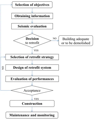
3.1  Performance-based retrofit program 49 

3.2  Retrofit strategy 54 

3.2.1  Global strengthening/stiffening 55 

3.2.2  Increasing of deformation capacity 56 

3.2.3  Reduction of seismic demand 57 

3.2.4  Existing procedures for selecting an optimal strategy 59 

3.3  Retrofit systems 63 

3.3.1  Global intervention techniques 63 

3.3.2  Local intervention techniques 68 

4.  Engineering application of Soft-Computing: a literature review 75 

4.1  Fuzzy logic 79 

4.1.1  Applications of FL in modeling problems 80  4.1.2  Applications of FL in simulation problems 80  4.1.3  Applications of FL in optimization problems 82 

4.2  Artificial Neural Networks 84 

4.2.1  Applications of ANN in modeling problems 85  4.2.2  Applications of ANN in simulation problems 88  4.2.3  Applications of ANN in optimization problems 89 

4.3  Evolutionary Computation 93 

4.3.1  Swarm Intelligence 94 

4.3.2  Evolutionary Algorithms 99 

5.  A Soft-Computing approach to seismic retrofitting 107 

5.1  Formulation of the optimization problem 107 

5.2  Optimization algorithms 111 

5.3  Simulation Framework 116 

5.3.1  Model Builder Object 117 

5.3.2  Domain Object 118 

5.3.3  Analysis Object 119 

5.3.4  Recorder Object 124 

5.4  Software Environment 124 

6.  Implementation of the Soft-Computing procedure 127 

6.1  Population representation and initialization 127  6.2  Creation of Finite Element Models (Pre-processing) 134 

6.2.1  Modeling of local intervention 137 

6.2.2  Modeling of global intervention 138 

6.3  Seismic analysis (Processing) 143 

6.4  Post-processing 147 

6.4.1  Evaluation of constraints 147 

6.4.2  Evaluation of the objective function 156 

6.4.3  Evaluation of the penalty 158 

6.5  Selection 161  6.6  Crossover 165  6.7  Mutation 168 

6.8  Convergence criteria 171 

6.9  Tuning of the GA parameters 172 

6.9.1  Proposal of fast tuning strategy 174 

6.10 Parallel computing 183 

7.  Applications 191 

7.1  The “case studies” 206 

7.1.1  The Finite Element Model for as built-configurations 207 

7.1.2  As-built conditions 210 

7.2  The outcomes of the procedure 218 

7.2.1  The optimal genotype 226 

7.2.2  The optimal phenotype 235 

7.2.3  The “retrofitted” condition 243 

8.  Concluding remarks and open issues 261 

8.1  Concluding remarks 261 

8.2  Reduction of CPU time 262 

8.2.1  Classifying the retrofit solutions through ANN 262 

8.2.2  Changing the hardware architecture 267 

8.3  Future developments 268 

8.3.1  Accurate seismic analysis 268 

8.3.2  Other retrofit systems 269 

8.3.3  Brittle mechanisms 270 

8.3.4  Architectural constraints 271 

8.3.5  Multi-objective function 273 

1.1 Motivation and objectives

The seismic risk generally means the expected loss in terms of lives injury, property damage, direct and indirect costs due to potential ground shaking associated with energy release from a fault for a given area and a reference period [1]. It is determined by a combination of earthquake hazard, vulnerability, and exposure. The greater or lesser presence of goods at risk and, therefore, the consequent possibility of suffering damage is defined as “exposure” (of human life, economic assets, and cultural heritage).

Earthquake hazard, also called “seismicity”, measures the likelihood that a seismic event of a given magnitude (or intensity) affects a certain area in a certain interval of time. Geological studies and historical records indicate that lower magnitude earthquakes generally occur more frequently than higher magnitude ones [2] [3] [4]. The ground motion at a site depends on the natural evolution of the earth's crust and, hence, seismicity is a physical characteristic of a certain area. The higher the seismicity, the higher the probability of earthquake occurrence in the same interval of time.

Moreover, vulnerability represents the building’s susceptibility to damage induced by the seismic event of a given magnitude (or, correspondingly, return period). In fact, the greater the vulnerability (among the other things, due to inadequate design, poor quality materials, construction methods, lack of maintenance as described in Section 1.2) the more serious damage the structure will suffer as a result of the induced seismic shaking [5].

However, the fault rupture that originates the earthquakes does not itself kill people or induce great economic losses. What causes most of the injury and economic losses is the interaction of the earthquake ground motions with the built environment. Seismic “disaster” at any site or region is, hence, the consequence of the interaction of the sources of potential earthquake hazards (created by the local seismic activity associated with energy release from a fault) with the vulnerability of the human-made facilities (either engineered or not). The economic loss induced

by earthquakes depends not only on their magnitude and on the surface propagation of the seismic waves but also on the level of “anthropization” of the affected areas and the human ability to build safe buildings and infrastructures.

That said, Italy is characterized by a medium-to-high seismicity due to the frequency and magnitude of the earthquake phenomena. In the last 150 years, there have been around 30 earthquakes with a destructive character. From the beginning of the 20th _{century, there have been 6 major earthquakes (Figure 1.1) with a} magnitude equal or higher than 6.5 causing a total number of casualties equal to 126,607 [6].

Messina 1908 (deaths: 85,926) Avezzano 1915 (deaths: 32,610)

Friuli 1976 (deaths: 989) Irpinia 1980 (deaths: 2,914)

L’Aquila 2009 (deaths: 309) Amatrice 2016 (deaths: 299)

The exposure in Italy stands at high values as a result of the high population density and the presence of an important historical, artistic and monumental heritage [7]. In this sense, it is significant the seismic event in Umbria and Marche occurred in 1997, which severely damaged 600 churches and, particularly, the Basilica of St. Francis of Assisi (Figure 1.2).

(a) (b) Figure 1.2: Damage to Basilica of St. Francis (a) and San Biagio Church (b)

Hence, Italy is one of the countries facing the highest seismic risk in the Mediterranean area. However, the ratio between occurred damage and the recorded amount of energy released during the events is much higher than other highly seismic countries. Italy with respect to those countries, where the earthquake hazard is even greater, is characterized by a very high vulnerability affecting constructions built even in the recent past and devoted to public and strategic purposes [8]. Some of them have been designed and consequently built prior to the entry into force of the first regulations for construction in the seismic area or in accordance to subsequently replaced or radically amended seismic regulations which over time, due to advancement in engineering knowledge, have improved the degree of analysis and considerably enhanced the magnitude of the design seismic forces [9]. The older buildings usually cannot comply with the more stringent specifications of the latest standards even if constructed in compliance with prevailing standards of the time. Other existing buildings are placed on sites whose seismicity has been upgraded after their construction.

The evolution of the seismic hazard assessment of Italian territories over the years and subsequent application of appropriate design rules have often led to seismic design actions higher than expected during the design stage [10] [11]. The following Table summarizes the time evolution of both seismic codes and hazard classification occurred in Italy during the last century.

Evolution of Italian seismic code Evolution of seismic classification R.D. 193, 1909 1 st generation standards purely prescriptive 1909 R.D. 143, 1909 No Zone R.D. 2089, 1924 R.D. 431, 1927 R.D. 431, 1927 Zone I – II R.D. 640, 1935 R.D. 2228, 1939 1950 Law n. 1684, 1962 C.M. 6090, 1969 Law n.64, 1974 2 nd generation standards 1-level performance D.M. 1975 D.M. 1981 D.M. 515 1981 Zone I – II - III D.M. 1984 D.M. 1986 D.M. 1996 Testo Unico 2001 2000 O.P.C.M. 3274, 2003 3

rd generation standards 2-levels performance

O.P.C.M. 3274, 2003 Zone I – II – III – IV O.P.C.M. 3431, 2005 D.M. 2005 D.M. 2008 [15] 4th _generation standards multi-levels 2010

According to the most recent seismic classification [12], 43.5% of the national territory is characterized by high earthquake hazard (seismic zone I or II). According to the 2011 Italian census [13], the number of buildings with a predominantly residential use shown in Table 1.1 is 12,180,131.

More than 35% of the residential buildings are placed in a high-risk area where 21.7 million people live. Particularly, the census states that reinforced concrete structures on which the present Ph.D. thesis is focused are rather spread in all the aforementioned seismic prone regions, representing the 33% of Italian built stock.

However, a percentage equal to 68% of existing residential buildings have been built before 1971 according to the 1st _{generation (purely prescriptive) standards.} Moreover, a percentage lower than 2% of homes were built in the years 2000 when technical standards began to impose far more restrictive criteria.

Table 1.1:Estimated number of homes with potential seismic risk [14]

Region

I generation

standards II generation standards III - IV generation standards _Total

< 1971 1972 - 2001 2002-2011 Abruzzo 193,488 95,891 3,808 293,187 Basilicata 88,184 40,417 1,571 130,172 Calabria 292,312 179,335 1,554 473,201 Campania 646,446 307,505 6,095 960,046 Emilia-Romagna 590,290 260,064 30,046 880,400 Friuli 185,350 81,753 6,258 273,361 Lazio 716,741 310,627 4,394 1,031,762 Liguria 419,296 63,939 1,508 484,743 Lombardia 1,287,572 525,336 52,320 1,865,228 Marche 202,243 93,341 7,419 303,003 Molise 62,613 21,436 1,163 85,212 Piemonte 849,156 210,936 6,607 1,066,699 Puglia 495,199 283,620 1,015 779,834 Sardegna 178,954 144,636 5,911 329,501 Sicilia 675,706 386,492 5,035 1,067,233 Toscana 623,183 174,037 15,958 813,178 Trentino 157,764 68,008 6,798 232,570 Umbria 111,188 53,881 5,671 170,740 Valle d'Aosta 31,994 13,333 1,023 46,350 Veneto 560,107 298,649 34,955 893,711 Total 8,367,786 3,613,236 199,109 12,180,131

Although recent progress have been done in the area of seismic prediction, the earthquakes cannot be accurately predicted in time, magnitude or location. Furthermore, despite earthquake resistance requirements in building codes have become more stringent and improved significantly even the last codes are not infallible [15]. Therefore, the main way of decreasing economic and life losses as a

direct consequence of earthquake disasters is making new building earthquake-safe and strengthen existing ones. Therefore, the need for strengthening existing buildings has emerged as a technical challenge [16] and a societal priority [17] as a result of the significant damages and casualties often deriving from seismic events.

Over the last seventy years, around 190 billion euros have been spent in post-event restoration and reconstruction including direct and indirect costs [18]. Retrofitting of vulnerable structures is a major task that many building corporations and government have to address. In future projection, the costs of securing the housing stock from earthquakes depend on the level of risk coverage that is deemed acceptable.

Based on this assumption, referring to the Italy’s housing stock and using as a parameter of seismic intensity the impact of the earthquake of L'Aquila [19] (representing, on the scale of historically recorded in Italy, an average destructive event), CNI’s Study Center has suggested a possible distribution of the intervention costs based on the age distribution of the buildings and their structural conditions [14]. According to this study, the percentage of structures to be retrofitted based on the examination of the damages recorded to houses in L'Aquila and the housing conditions gathered from census surveys is equal to approximately 40% of houses in the country, regardless of the seismic risk level.

In this perspective, about 12 million properties (with a population of around 23 million people involved) should be involved in rehabilitation and static safety intervention. Applying the average parameters of technical specifications for seismic interventions, there would be an overall cost to secure the Italians’ housing stock by average seismic events of about 93 billion euros (Table 1.2). Hence, the financial implication of such a huge task could be mind-boggling.

Nowadays, no well-established and completely accepted procedures are available for obtaining the optimal seismic retrofitting solution. Therefore, the definition of a rational strategy for seismic retrofitting is still an open issue. In the Authors’ best knowledge, no relevant study is currently available for approaching seismic retrofitting of existing RC frames as an optimization problem, as recent scientific contributions on optimization algorithms are restricted to seismic design of new structures [20][21].

Conversely, in the current practice, as well as in most relevant scientific contributions on this topic [22]-[26], seismic retrofitting of RC frames are only based on common sense. Considerations about optimization are left to the engineering judgment and, hence, they are not part of a systematic analysis. This is partly due to the complexity of the constrained optimization problem under

consideration, which cannot be duly approached by means of analytical techniques commonly employed in structural engineering, as it can only be solved by means of alternative techniques that are not in the background of common structural engineers.

Table 1.2:Cost estimate necessary to make Italian homes safe from seismic risk [14]

Region Seismic _{zone 1} Seismic _{zone 2} Seismic _{zone 3} Seismic _{zone 4} Total [€]

Abruzzo 519,608,951 956,819,990 1,026,708,276 - 2,503,137,217 Basilicata 389,756,074 578,689,566 110,593,193 - 1,079,038,833 Calabria 2,261,606,036 1,674,589,040 - - 3,936,195,076 Campania 757,085,265 6,495,980,770 842,691,565 - 8,095,757,600 Emilia-R. - 1,886,802,360 4,444,537,374 360,037,192 6,691,376,926 Friuli 175,023,026 912,238,866 282,330,683 668,360,083 2,037,952,658 Lazio 289,653,340 2,251,614,507 4,944,840,424 188,586,014 7,674,694,285 Liguria - 358,830,381 978,983,635 1,978,397,589 3,316,211,605 Lombardia - 244,134,343 2,127,065,643 10,530,581,244 12,901,781,230 Marche 21,979,822 2,286,865,047 145,423,612 1,608,381 2,455,876,862 Molise 180,286,210 473,637,420 94,327,642 - 748251272 Piemonte - 259,827,928 726,379,390 6,400,791,351 7,386,998,669 Puglia 82,257,196 1,206,391,434 2,125,295,858 2,952,326,318 6,366,270,806 Sardegna - - - 2,376,413,502 2,376,413,502 Sicilia 562,630,213 7,477,470,927 11,386,789 637,807,857 8,689,295,786 Toscana - 1,264,897,651 5,031,170,932 475,004,478 6,771,073,061 Trentino - - 272,053,211 1,128,520,230 1,400,573,441 Umbria 238,681,660 1,054,306,951 230,937,694 27,123,598 1,551,049,903 Valle d'A. - - 37,820,498 264,450,404 302,270,902 Veneto - 929,716,300 3,857,865,949 2,497,349,972 7,284,932,221 Total 5,478,567,793 30,312,813,481 27,290,412,368 30,487,358,213 93,569,151,855

Therefore, this Ph.D. Thesis proposes a soft-computing (Chapter 4) approach capable of selecting and designing the “best” solution (in terms of initial costs) for seismic retrofitting of existing RC buildings.

1.2 Common deficiencies in existing R.C. buildings

Recent devastating earthquakes [27]-[31] have evidenced the vulnerability of many existing reinforced concrete buildings. The seismic vulnerability mainly depends on the seismic deficiency of the building under consideration, which, in turn, is defined as a condition that prevents a building from meeting the required performance. These deficiencies have a strong influence on the potential damage and modes of failure of components during an earthquake when directly affects the structure’s ability to sustain the seismic loads and remain stable. More than any

laboratory test or analytic study, the lessons learned from past earthquakes should serve to establish a historical record of what worked well in past earthquakes, as well as what did not.

Damage investigations have demonstrated the poor performance of older buildings designed using out-dated technology. The most important and the most frequently observed deficiencies that have been found to have negative consequences for seismic behavior can be taken as a reference to learn from past mistakes and avoid them in the future. A wide, yet not-exhaustive, list of critical deficiencies contributing to the vulnerability of concrete buildings is proposed in the following subsections. For convenience, the deficiencies have been broadly classified as follows: local deficiencies, when they refer to the deficiencies in individual members, and global deficiencies, when they refer to the deficiencies which are observed in the structure as a whole [32]. Finally, even the common mistakes made in analysis and concrete mixing are described.

1.2.1 Component deficiencies

Component (or local) deficiencies typically include the poor detailing of single structural members or connection between them, the inadequate sizing of cross sections or steel reinforcement and so on. Consequently, the structural members are not able to behave properly under seismic actions.

1.2.1.1 Deficiencies of columns

During an earthquake, columns of frame buildings may fail under shear-compression or bending-shear-compression force. It is often difficult to distinguish such mechanisms, as both failures take place near the column ends and involve concrete crushing. However, shear failure is a result of the opening of diagonal cracks and degradation of the shear transfer mechanism, which is associated with low energy dissipation and sudden failure also known as “brittle failure”.

The tensile stresses carried by the concrete before the onset of significant shear cracking cannot be resisted by shear reinforcement once shear cracks open, leading to diagonal tension failure. Further opening of cracks and movement along the diagonal failure plane, in the case of high axial loads and inadequate stirrups, can lead to loss of gravity load-carrying capacity, accompanied by buckling of longitudinal reinforcing bars. As axial capacity is lost, gravity loads should be transferred to neighboring columns, which can lead to a progression of overload, damage and eventually collapse of the buildings.

This type of failure occurs due to several reasons, such as the widely spaced horizontal ties laid in the column, the low strength of shear reinforcement, the reduction in steel area due to corrosion, the inadequate cross-section size of the column (Figure 1.3a). Moreover, if the ends of rectilinear lateral reinforcement are not properly anchored in the core concrete with a bend it may lead to shear failure of columns by pull-out of lateral reinforcement from the anchorage zone (Figure 1.3b).

Another type of shear failure may be caused by interaction with masonry infills during an earthquake. In fact, columns next to openings or short (and stiff) columns, due to infill walls of partial height (Figure 1.3c), attract larger shear force which leads to their failure prior to flexural yielding at their ends because of reinforcement not properly done.

(a) (b) (c) Figure 1.3: a) Corroded re-bars; b) inadequate stirrups [33]; c) short column

If short and tall columns exist within the same story level, then the “short columns” [34] attract several times larger earthquake-induced force and suffer more damage as compared to taller ones. The negative effect can be caused by the free inflection length reduced by the presence of infills for a partial height that acts as a constraint where it is present, subjecting the column to shear stresses only into the short free length. The “short column” effect can also happen when the effective height of some columns in a particular story is reduced by the presence of an intermediate floor.

Bending (or flexural) failure, whereas, may occur either due to the premature crushing of concrete in compression or due to yielding of steel, accompanied by tensile cracking of concrete. Bending failures usually occur because of an inadequate amount of steel bars provided vertically in the columns, inadequate amount of lateral reinforcement, particularly near the beam-column joints or column-foundation junctions, namely the region of plastic deformation. Finally, columns with a large aspect ratio (length to width ratio) are often inadequate under biaxial bending forces.

1.2.1.2 Deficiencies of beams

Under gravitational loads, the beams typically sag in the middle and hog near the column supports, generating a flexural crack pattern in beam span. On the contrary, under seismic conditions, this hogging action increases at one end, but decreases and sometimes reverses to sagging at the other end. The pre-existing cracks may be opened further because of the effects of the vertical component of the earthquake.

During an earthquake, the beams may also fail either in shear or in bending (flexural failure), but their failure is less “catastrophic” than the failure of a column: in contrast to failure of a column which can affect the stability of the whole building, the failure of a beam causes a localized effect. However, shear (brittle) failure is always undesirable, as it decreases the load resisting capacity and prevents the yielding of the longitudinal steel bars (ductile behavior).

These failures mainly occur because of the absence of proper detailing. In fact, the lack of proper stirrup spacing (nearly equal to the beam depth) often designed for gravity shear loads along with the use of smooth longitudinal steel bars can generate the formation of shear cracks that led to a reduction in both flexural and shear strength.

Bending failures often occur because of the poor quality of concrete, inadequate amount of horizontal steel bars, or inadequate anchorage of the re-bars, particularly near the beam-column joints, or. In fact, the yielding of the re-bars under reversed cyclic loading increases the rotation near a beam-column joint, resulting in the formation of the so-called “plastic hinge” that plays a significant role in the seismic response of structures for the dissipation of internal energy. The rotation capacity of a beam near the joint may be inadequate due to lack of confining reinforcement. In fact, the amount of hoops near the joints is often such that the beam doesn’t generate their rotation (flexural) capacity before they fail in shear. This may lead to a sudden shear failure before a hinge is formed (Figure 1.4).

 

 

   

Figure 1.4: Example of shear failure in the beam [35]

1.2.1.3 Deficiencies in the beam-column joints

Joints between beams and columns play an important role: their integrity ensures that beams can safely transfer forces to columns and columns, in turn, can transfer forces to foundations. However, in existing frames, beam-column joints (also called “panel zone”) sometimes lack adequate confinement and transverse reinforcement (Figure 1.5a).

It is also very common to find eccentric beam-column connections usually located in the perimeters of moment frames structures. In existing structures, top bars have often hooks bent upward, while bottom bars are typically discontinued at the face of the supporting column (anchored in essentially plain concrete) or provided with only a short embedment into the joint. This is in contrast to the preferred detailing for beam longitudinal reinforcement of extending the top and bottom bars through beam-column joints with hooks bending into the joint.

 

 

(a) (b) Figure 1.5: a) Poor beam-column connection; b) failure of a corner joint

In case of a moment-resisting frame characterized by “weak-beam strong-column behavior”, the weak detailed joint after the yielding of the beam is not able

to develop the strength of the connected members. Such deficiencies could lead to axial and/or sudden shear failure of the panel zone characterized by diagonal cracking which results in redistribution of gravity loads to neighboring joints (and columns), reduction of the stiffness and progressive collapse of the building.

In principle, interior joints are less vulnerable due to the confinement provided by four beams connected to the column. On the contrary, the corner joints around the building perimeter are usually more prone to fail, as shown in Figure 1.5b. 1.2.1.4 Deficiency of frames

As known, in the 3D configuration of a framed structure, only the frames aligned in one direction form a lateral-force-resisting system capable to react to seismic loads acting in the same direction. However, if the existing buildings were designed to resist only to gravity loads, they generally are not characterized by a specific lateral-force-resisting system.

The presence of frames in one direction and the mono-directional warping of the floors are typical of buildings designed according to the past seismic codes: for designing buildings in non-seismic areas the engineer had to account only the vertical loads. In such cases, sometimes transverse beams (i.e. placed in the frames on which the floor does not directly rest) are completely absent or have very small size. In this situation, the resistance to lateral actions in the direction parallel to the joist is very low. Therefore, under moderate to a large earthquake, the overall lateral resisting strength and stiffness are often inadequate to limit story drifts and/or to resist additional demand due to earthquake loading. Excessive horizontal displacements generate P- effects, thus, impairing the global stability of the frame.

Another deficiency can be due to low structural redundancy, i.e. the ability to redistributed overstress by creating alternative load paths. In the lack of redundancy in a structure, the seismic capacity is mostly dependent on the nonlinear behavior of the lateral load resisting elements. Finally, in curved buildings with non-rectangular grid plans, the frames are not parallel or symmetric about the major orthogonal axes of the seismic force resisting system. This leads to decreasing the lateral strength of the building.

1.2.1.5 Deficiencies of foundations

Foundation deficiencies can occur within the foundation element itself, or due to inadequate transfer mechanisms between foundation and soil. Element deficiencies include inadequate bending or shear strength of spread foundations, inadequate

axial capacity or detailing of isolated foundation system. On the other hand, the overall stability of a building depends, among the others, on the transfer mechanism of the supported loads to the soil (or rock). A deficient transfer of loads to the foundation system often causes an inappropriate behavior of the structure leading to several damages. Many existing structures were built upon isolated footings, not properly designed against seismic forces.

Other dangerous situations occur when the deformations or volume variation of the soil are not caused by the load. It is the case of the building placed on poorly compacted or water-sensitive soil that may result in loss of bearing capacity, uniform or differential settlements and, consequently, in large uniform or differential displacement.

The so-called “liquefaction” phenomenon occurs when a saturated or partially saturated soil substantially loses strength and stiffness in response to sudden change in stress condition (due to earthquake shaking), causing it to behave like a liquid. The earthquake (or other cyclic) loading reduces the soil volume and develops pore water pressure. This reduces the effective stress to zero and the soil cannot support a structure (Figure 1.6a).

The soil liquefaction sometimes is also the cause of the occurrence of global “overturning” mechanism of many multi-story buildings during the earthquake (Figure 1.6b), which results in the excessive rotation. This failure mode happens when the moment at the base of a building due to the lateral seismic forces is larger than the resistance provided by the foundation’s uplift resistance and building weight. The global overturning mechanism results in high tensile or compressive forces in the vertical member located close to the end of the lateral force resisting systems.

 

(a) (b) Figure 1.6: Example of a) liquefaction of soil; b) overturning mechanism

Sometimes damages may be caused also by the presence of heterogeneous foundation systems on heterogeneous soils. In other cases the construction of large buildings nearby existing frame structures causes the intersection of stresses “bulbs”, increasing the settlements in that area.

Another observed source of damage is the construction of additional stories upon weak columns, instead of enhancing the existing foundation system. The load increment usually lead to loss of bearing capacity and/or compaction of soil foundation.

1.2.2 System deficiencies

System (or global) deficiencies are the attributes responsible for degradation of the lateral load resisting mechanism of a building subjected to an earthquake. Typically, such deficiencies are caused by “irregularities” in the structural configuration which result in an irregular load path, damage and eventually failure of the structure.

They are generally classified in plan and vertical irregularities [36]. Both are important factors that decrease the seismic performance of the structures and can result in significant increase of loads and deformations in comparison to those assumed by the conventional linear methods of analysis. The irregularities are broadly classified as plan irregularities and vertical irregularities. The section list the different types of irregular configuration.

1.2.2.1 Plan Irregularities

The plan irregularities can be detected by observation and simple calculations based on the plan of a building. Sever plan irregularities can result in dynamic behavior governed by torsion, leading to large displacement demands and collapse on the “soft” or “weak” side of the building.

The existence of an asymmetric in-plan configuration (e.g. T, L or U-shaped plans) without seismic joints or the asymmetric (or even non-parallel) existence of lateral force-resisting elements are usually leading to an increase in stresses of certain elements that consequently results in a significant damage during an earthquake. Such category includes torsional irregularity, diaphragm inadequacy, and out-of-plane offsets.

1.2.2.1.1 Torsional irregularity

In a multi-story structure, seismic force at each level acts through its center-of-mass and is resisted by the building through resulting shear force applied in the center-of-rigidity of its frames. Centre-of-mass is the point of each floor where the mass of the floor and tributary portions of the adjacent stories can be considered to be lumped for the purpose of analysis. Centre-of-rigidity (or stiffness), whereas, can be identified for each floor as the point such that when the horizontal force along a direction acts at that point, the resulting displacement of the level is a pure translation in the same direction.

Torsional irregularity is caused by plan asymmetry and/or eccentricity between these centers. This is usually due to a particular in-plan configuration, such as the asymmetric in-plan distribution of lateral stiffness or the asymmetrical position of stairs and/or lift, that leads to twisting of the building and increased shear forces especially in the in members away from the center of rigidity (that is on the “flexible side”). Because of torsional effects, different portions of the same floor move horizontally by different amounts and this induces larger damage (higher inelastic demands) in the exterior columns and walls.

This problem is especially common in buildings at the corner of a block, where common walls as the back of the building provide large resistance while the street sides provide less resistance. Another example occurs in office buildings in which an elevator hall surrounded by structural walls may be placed on one side of the floor to leave large open office area in the remainder of the floor.

1.2.2.1.2 Diaphragm inadequacy

Structural diaphragms are required to span between vertical elements of the lateral-force-resisting system and, thus, to transfer forces in the horizontal plane. A rigid floor slab acts as a horizontal diaphragm that mobilizes the frames to resist the lateral load and to undergo the same displacement at the floor level.

A diaphragm discontinuity refers to a large cut-out or open areas in a floor slab which generates stress concentration in the corners of the cut-out. Large openings in floor diaphragms (usually greater than 50% of the gross enclosed diaphragm area) due, for instance, to the presence of stairwells and/or lift are considered structural deficiency.

As consequence of this deficiency, the diaphragm action of the slab may be reduced and the global behavior of the existing building could be inadequate. Moreover, buildings having diaphragms that span large distances between vertical

elements of the lateral-force-resisting system usually become overstressed in moment or shear, leading to unexpected inelastic behavior in the diaphragm. 1.2.2.1.3 Out-of-plane offsets

The out-of-plane offset refers to the discontinuity (or interruption) of the lateral load resisting systems which are shifted within their own plane in a certain story.

An example is a peripheral column in the upper stories that is interrupted at the ground floor. In this case, the columns are supported on cantilever overhang beams and they are termed as “floating” columns. This leads to a discontinuity in load path from the perimeter frame in the upper stories to the outer columns in the ground story.

This deficiency usually occurs when there is a limitation for moving space along the border of the building at ground level. This type of frame may be adequate for gravity loads but perform poorly when subjected to earthquakes. 1.2.2.2 Vertical Irregularity

The vertical irregularities can be detected by observation and simple calculations based on the elevation of a building profile. Discontinuity of vertical elements in the seismic-force-resisting system can result in excessive earthquake-induced deformations and force demands concentrate just above the vertical irregularity.

Such category includes geometric irregularity, mass irregularity, stiffness irregularity, strength irregularity, and deficiency in separation joints

1.2.2.2.1 Geometric irregularity

A geometric irregularity generally occurs with “setback buildings”, where the horizontal dimension of the story is greater than the adjacent one. An example of setback building can be found in existing building with a small appendage, such as a penthouse, at the upper levels. Such configuration can cause large deformation just above the setback during an earthquake.

1.2.2.2.2 Stiffness irregularity

Stiffness irregularity refers to the variation in terms of lateral stiffness between consecutive levels. The substantial reduction in lateral stiffness in any story with respect to that in the upper story may lead to a “soft story” failure.

A soft story is a relatively flexible story in which its relative horizontal displacement is much larger than the corresponding displacements of other stories.

This mechanism is highly undesirable because significantly increases the deformation demand and puts the burden of energy dissipation concentrated on the columns of the same level, with almost irrelevant damage to the remaining part of the building (both lower and upper floors).

As a matter of fact, if the columns have not been well detailed, or in case of large axial forces (particularly at ground-story), the columns are unable to follow the large story drift without failure (Figure 1.7a).

Soft stories are especially common in multi-story residential buildings where the infill walls, which affect the stiffness of the story, are absent to meet the change in use. In this case, the first story often is used for “open space” (like the “pilotis” configuration), commercial facilities or garages. Moreover, soft intermediate stories have also been observed in buildings with large windows on the façade (Figure 1.7b).

(a) (b) Figure 1.7: Example of a) ground soft story; b) soft intermediate story

1.2.2.2.3 Strength irregularity

The strength irregularity refers to substantial discontinuity in terms of lateral strength in any story with respect to the upper story. The story strength is the total strength of all seismic-resisting elements sharing the story shear for the direction under consideration. Inadequate story shear strength caused by an insufficient number of columns and/or walls is referred to as “weak story”.

Figure 1.8a shows an example of weak story mechanism that usually occurs in buildings with an “open” story at the first floor, while infill or structural walls in the upper stories. Moreover, it can also occur in many residential buildings characterized by massive beams and smaller designed columns (also called ‘‘weak

column-strong beam’’) in which yielding mechanism of columns is possible at any story.

The weak story can lead to an undesirable “sway” mechanism under seismic load and, eventually, in “pancake” failure (Figure 1.8b). The sway mechanism generally refers to the movement of the upper stories like a single block with severe deformation of the ground story columns. The process results in a concentration of inelastic deformation demands in the columns of one story which are exacerbated by P- effects in taller buildings.

(a) (b) Figure 1.8: Example of a) weak story; b) pancake failure

1.2.2.2.4 Mass irregularity

Existing buildings are sometimes used for a different purpose from their original intended function. The observed substantial difference in mass (or weight) between two consecutive stories due to heavy equipment in a particular floor is accounted in this category. The concentration of mass at a particular story attracts higher seismic forces and generally results in the creation of a “weak” story.

1.2.2.2.5 Deficiency in separation joints

Inadequate separation joints (gap) between two adjacent buildings, especially those with different heights, different materials, different dynamic properties and free to oscillate independently, may lead to “pounding” (or “hammering”) mechanism when they collide between them during the vibration (Figure 1.9a).

This condition is particularly adverse when the floor levels of the adjacent buildings do not match. If the floor slabs of adjacent buildings do not line up horizontally, the top slab of the shorter building can severely damage the columns of the adjacent building leading to axial load failure due to excessive demands

caused by dynamic horizontal vibrations of the two buildings. This mechanism is called “mid-column” pounding whose example is shown in Figure 1.9b.

On the other hand, if the buildings are located within in a block of similar height buildings, collapse due to pounding is less likely to occur since differential movement and dynamic effects are “constrained” by the presence of the adjacent structures.

 

 

(a) (b) Figure 1.9: Example of a) pounding mechanism [33]; b) mid-column pounding 

1.2.3 Deficiencies in concrete mixing and placement

Due to insufficient mixing, placement, and workmanship, the compressive strength of concrete is often smaller than half of the expected strength. In order to achieve workability, the water-cement ratio is usually exceeded compromising the strength of concrete [37].

Quality and shape (mostly rounded) of fine and coarse aggregates can lead to low stiffness and improper binding of concrete [38]. In addition, aggregate dimensions used in the concrete are sometimes larger than the allowable diameter: segregation and bleeding have been commonly observed in the damaged buildings in the seismic-affected area.

The aging of materials and aggressive environmental conditions can unavoidably lead to their deterioration with an adverse effect on the potential seismic performance of a building [39]. In addition, the inadequate bar cover, poor or cracked concrete may cause moisture and oxygen to penetrate to the steel reinforcement leading to its corrosion. Another source of deficiency has been found in many existing frames built in stages: the non-homogenous and non-monolithic construction can lead to a variation in terms of structural performance.

1.2.4 Deficiencies in analysis

The most important source of deficiency in the analysis is related to the acting loads. Existing buildings have been often designed to resist under gravity loads, while the seismic loads have been underestimated or completely neglected in the analysis.

Moreover, practitioners usually do not take into account the modifications to the structural system happened for functional reasons over time. Both addition and removal of elements commonly observed in existing building result in significant increases in dead and live loads which are sometimes neglected in the analysis.

As regards the nonstructural elements, despite they are placed for the purpose of building function (the case of partition walls), they are commonly neglected in the analysis for design calculations. For instance, the contribution of unreinforced masonry in infill walls is often neglected in the analysis leading to a longer time period and, as consequence, lower seismic forces [40]. Although the infill walls are not designed to absorb seismic actions, actually they can absorb still part of these actions in proportion to their stiffness and affect the shear resistance of the story. Moreover, the stiffness of an infill wall can influences also the location of the center of rigidity of the lateral load resisting system in a story. For instance, if infill walls are present only on one side, neglecting them analysis may lead to overlooking a torsional irregularity.

On the one hand, damage occurring in infill wall could contribute to the dissipation of input energy and reduce the seismic forces on the frame. On the other hand, when stiff and strong nonstructural elements are placed in contact with structural elements the interaction can result also in structural element damage. In the examples of Figure 1.10 a-b, the compressed rod forming in the wall acts in a concentrated area of the frame where it may cause brittle failure in the columns.

   

(a) (b) Figure 1.10: Example of a) interaction with the column; b) diagonal rod in infill wall

Moreover, the engineer sometimes did not account for the P-∆ effect in the analysis. This effect is due to the increase of lateral displacement response of structure during the seismic event which leads to a higher eccentricity of the vertical loads, causing additional moment in the columns. Neglecting this effect can result in the under-estimation of the design forces.

Regarding the foundation system, whereas, it is sometimes designed without adequate information on geotechnical data such as the type of soil, bearing capacity, locations of fill and fault. Therefore, the amplification effects due to the interference of the earthquake waves are neglected in the analysis.

2.

State of practice on seismic analysis for design and

assessment

2.1 Simulation process

Seismic analysis of structures is a typical example of simulation problem, in which both earthquake-induced actions and mechanical properties of structural components are known and the mechanical response of the system is searched for.

Key issues in simulation include the acquisition of valid source information about the relevant properties of materials and models, the use of simplifying approximations and assumptions, and the validation results. Figure 2.1 shows the main steps characterizing the simulation problem are idealization, discretization, and solution.

Figure 2.1: A simplified view of the physical simulation process

2.1.1 Idealization

Engineering systems often tend to be highly complex. Hence, for simulation, it is necessary to reduce that complexity to manageable proportions by developing a reasonably simplified model intended to predict the key characteristics and aspects of the selected system’s behavior. Complexity reduction can be achieved by filtering out the physical details of the system that are not relevant to the analysis process. Engineers often approach the simulation problem intuitively by creating an analogy between the real world and the simplified system.

The idealization is a simplifying process by which an engineer passes from the real system to its mathematical model. Hence, idealization is an abstraction tool by which complexity is tamed. It is the most important step in engineering practice because it must be done by humans. Models introduce approximations and

Real World Simplified system Mathematical Model Discretized Model (Mesh) Discrete Solution Solution Discretization Idealization

assumptions, but allow the description of a property over a wide range which cannot be covered by real data.

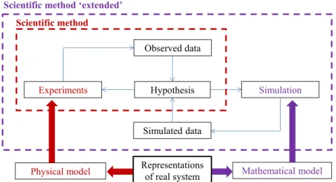
According to an “extension” of the scientific method whose flow-chart is shown in Figure 2.2, mathematical models allow exploring system behavior in an articulated way which is often either impossible or too risky in the real world. Mathematical models also enable the search for conditions outside the range of known properties.

Figure 2.2: Flow-chart of scientific method based on a mathematical model

Two types of models can be distinguished: rather simple equations, where parameters are fitted to experimental data, and predictive methods, where properties are estimated. The equations are normally preferred because they describe the property almost exactly. To obtain reliable parameters it is necessary to have experimental data which are usually derived from data banks or from measurements.

Despite using predictive methods is much cheaper than experimental work, predicted properties are normally only used in early steps of simulation because these estimation methods normally introduce higher errors than equations (or correlation) obtained from real data.

Moreover, the modeling can be further divided into implicit or explicit modeling. The former means choosing a specific component system from a “catalog” which automatically implies fully aware of the choice (including the mathematical models on which the component are based). The other extreme is explicit modeling: a mathematical model of the physical problem is selected on the basis of own technical expertise, resources, and maturity.

Observed data

Hypothesis

Simulated data

Simulation

Experiments

Physical model Representations_{of real system} Mathematical model

Scientific method

2.1.2 Discretization

In “continuous” systems the simulation problem can only be defined by using coupled partial differential equations in space and time subject to boundary and/or interface conditions which imply a huge number of unknowns (degrees of freedom). However, since the capacity of all computers is limited, the models of continuous systems can be solved by mathematical manipulation: it is necessary to reduce the number of unknowns to a finite number.

The process of sub-dividing a system into its individual well-defined components, whose behavior is readily understood, and then assemble the original system from a finite number components is called “discretization” (or “meshing”). This approximation approaches in the limit the true continuum solution as the number of components increases. The basic concept of discretization is the subdivision of the mathematical model into a finite number of disjoint components of simple geometry (Table 2.1) whose behavior is expressed in terms of a finite number of degrees of freedom.

Table 2.1:Typical element geometry defined by nodal location [41]

1D element 2D element 3D element

The response of the mathematical model of the complete system is then considered to be approximated by the response of the discrete model obtained by assembling the collection of all elements.

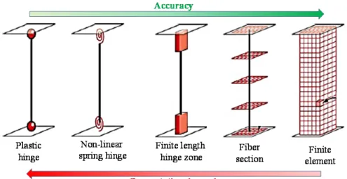
In particular, two main discretization strategies characterized by an increasing level of accuracy and complexity can be employed in the analysis of structures [42]:

 discrete finite element models, where a structural model is obtained through the assembly of a reasonable number of interconnected members;  microscopic finite element models, where members and joints are modeled

through a large number of two or three-dimensional elements connected between each other [43][44].

On the one hand, microscopic models are typically suitable for the detailed study of critical regions as a result of its complication and high-cost computational process. On the other hand, member element models often guarantee the best balance between simplicity and accuracy.

2.1.3 Solution

Analytical solutions (also called “closed-form solutions”) tend to be restricted to very simple problems of regular geometries with simple boundary conditions. Practical problems either do not yield to analytical treatment or the domain is geometrically complex and the likelihood of obtaining an exact analytical solution is very low.

Once formulated, the resulting mathematical models can be often hard to solve, especially when the governing equations are nonlinear partial differential equations. Alternatively, approximate solutions based on numerical methods are most often obtained in engineering analyses of complex problems (Figure 2.3).

Figure 2.3: Classification of solution methods for a mathematical model

Nowadays, the Finite Element Method (FEM) [45] is considered as one of the most powerful numerical methods for obtaining approximate solutions with good accuracy of complex boundary value (or field) problems in different fields of engineering.

A boundary value problem is a mathematical problem in which one or more dependent variables must satisfy a differential equation everywhere within a known domain and specific conditions on the boundary of the domain. The field is the domain of interest and most often represents a physical structure, while the field variables are the dependent variables of interest governed by the differential equation.

Methods

Analytical Numerical

Exact Approximate Numerical

solution

FEM method

The FEM solution process consists of the following steps:

1) discretization of the structure domain into regular finite elements with nodes (specific points at which the value of the field variable is to be explicitly calculated);

2) assembly of the elements at the nodes to form an approximate system of equations for the whole structure;

3) solving of the system of equations involving unknown values of the primary field variables (such as the displacements) at the nodes;

4) computation of desired additional quantities (derived variables) at selected elements.

The software executing the calculations is termed “solver” because it solves a set of mathematical equations for each node of the “meshed” model. It is worth highlighting that the way of assembling finite elements should ensure the following conditions:

 the field variables at the shared node of adjacent finite elements are equal (compatibility requirement);

 the elemental forces are in equilibrium with the external forces applied to the system nodes (equilibrium requirement);

 the system satisfies the boundary constraints (boundary conditions). The constraints are fixed values of the field variables (or their derivatives) on the boundaries of the field. Moreover, the values of the field variable computed at the nodes are used to approximate the values at non-nodal points (in the element interior) by interpolation of the nodal values. The interpolation functions, also known as “shape” (or blending) functions, are most often predetermined polynomial functions of the independent variables, derived to satisfy certain required conditions at the nodes and can be expressed by the displacement field of the real problem [46][47][48].

Based on the law of conservation of energy, the Finite Element Method has to solve the energy balance to find a stable operating point for the examined system. This is based on the Principle of Virtual Works which postulates that if a particle is under equilibrium, the work done by internal forces must be equal to the work done by the external forces acting on it. The FEM obtains the solution of desired field variables by minimizing the total potential energy of the discretized structure which can be expressed as follows:







   Γ T Ω T Ω T_{εdV d bdV d qdS} σ 2 1 Π _(2.1)

where  and  are the vectors of the stress and strain components at any point, respectively, d is the vector of displacement at any point, b is the vector of body force components per unit volume, and q is the vector of applied surface force components at any surface point.

The volume and surface integrals are defined over the entire domain of the system  and that part of its boundary subject to load . The first term on the right-hand side of this equation represents the internal strain energy, while the second and third terms are, respectively, the potential energy contributions of the body force loads and distributed surface loads.

However, the displacement is assumed to have unknown values only at the nodal points, and the variation within the element can be described in terms of the nodal values by means of interpolation functions. Thus, within any single element, the displacement d can be replaced by N u, where N is the matrix of interpolation functions and u is the vector of unknown nodal displacements. Likewise, the strains within the element can be expressed in terms of the element nodal displacements as  = B u where B is the strain displacement matrix. Finally, the stresses may be related to the strains by use of an elasticity matrix (e.g., Young’s modulus) as  = E .

The total potential energy of the discretized structure is the sum of all the energy contributions associated with each individual finite element which is given by the following equation (Eq. 2.2):





_

_



   Γ T T Ω T T Ω T T T e u B EB udV u N udV u N qdS 2 1 Π e e (2.2) Applying the principle of minimum potential energy, the stable operating point is found by setting the derivative of the functional with respect to the unknown displacement equal to zero (Eq. 2.3).



B EB



udV u N udV u N qdS 0 u 2 1 u Π Γ T T Ω T T Ω T T T e e e      







(2.3)

u k

f   (2.4)

where the term f represents the mechanical force (Eq. 2.5):





  Γ T Ω T_{udV N qdS} N f e (2.5) and k is known as the finite element stiffness matrix (Eq. 2.6)







 e Ω T T_{EB udV} B 2 1 k _(2.6)

However, for nonlinear problems, the stiffness matrix of a finite element depends on the actual displacements intensity and Eq. (2.4) must be reformulated as:

 

u u

k

f   (2.7)

On the one hand, the stiffness matrix of the whole system is nothing more than the summation of each element stiffness matrix. Likewise, the summation of load integrals yields the applied load vector.

Finally, there are two major methods for improving the accuracy of the solution. The aim of both methods is to obtain solutions that exhibit asymptotic convergence to values representing the exact solution. In the first method, the number of elements used to model a given domain is increased and, consequently, the finite element size is reduced (fine meshing).

Element type, size, shape, and quality have a big effect on the accuracy of the results: the more elements, the more accurate the results, but with a longer computational time analysis. In the second method, element size is unchanged but the order of the polynomials used as interpolation functions is increased.

2.2 Methods of analysis

Both Eurocode 8 [9] and Italian Seismic Code [15] allow to assess the seismic performance of a given structure on the base of the following linear and nonlinear methods:

 Linear Static analysis;  Linear Dynamic analysis;

 Non-Linear Static analysis;  Non-Linear Dynamic analysis.

The complexity of the procedure and the required computational “cost” are generally increasing in the list above: the Linear Static procedure is the easiest and quickest method, while the Non-Linear Dynamic procedure is the most accurate and computation intensive. Conversely, the computational effort decreases as complexity increases as shown in Figure 2.4.

Nowadays, the linear methods are permitted only in few cases, because the conditions for their applicability are very restrictive. They are mainly applied to the design of new structures.

Figure 2.4:Accuracy vs computational speed of most common methods of seismic analysis

According to both Eurocode 8 [9] and Italian Seismic Code [15], the need for accuracy in predicting the building’s internal forces and deformations together with the need of simulating particular case of extreme seismic loading direct the structural engineer into using non-linear analysis methods which have widespread applicability mainly in the assessment of existing structures. In fact, non-linear modeling and analysis allow more accurate determination of global capacity and ductility of the structure. The above-mentioned methods will be better discussed in the following Sections pointing out their relevant advantages and limitations.

2.2.1 Linear static analysis

The Linear Static Analysis (LSA) is the simplest method of seismic analysis. The term “static” means that the effect of seismic shaking is simulated by a system of forces constantly applied to the structural model. Linearity comes from the basic hypothesis of the methods: small deformations and elastic material. It implies a linear equation defining the relationship between loads and displacements.

In a linear static procedure, the building is modeled as an equivalent Single-Degree-of-Freedom (SDoF) system with an elastic stiffness and an equivalent viscous damping consistent with components responding at near yield level. The

Linear Static Analysis Non-Linear Static Analysis Linear Dynamic Analysis Non-Linear Dynamic Analysis Accuracy Computational speed

seismic input is modeled by a set of equivalent lateral static forces applied at the center of the mass in horizontal directions with the aim to produce the same stresses and strains caused by the earthquake they represent. The purpose is to simulate the peak inertia loads due to the horizontal component of the seismic action.

Based on an empirical estimation of the first fundamental period [49][50][51], engineers can calculate the seismic acceleration by mean a given Response Spectrum. The Response Spectrum is a plot of the peak or steady-state response (displacement, velocity or acceleration) of a series of SDoF oscillators of varying natural frequency, that are forced to a motion by the same base vibration. Once known, the seismic acceleration is multiplied by the mass of the building to calculate the equivalent static forces. The lateral shear force is then distributed over the height of the building assuming that the deformed shape associated with the 1st vibration mode is linear.

If the system responds basically elastically to the applied loads, the evaluated internal forces can be considered reasonable approximations of those expected during the design earthquake. As already seen, the linear static procedures are used primarily for design purposes. However, their applicability is restricted to regular buildings for which the 1st _{mode of vibrating is dominant.}

2.2.2 Linear Dynamic analysis

Linear Dynamic Analysis (LDA) removes some of the limitations of LSA and it is nowadays applicable for calculating the linear response of complex structures. Engineers have to model the building as a Multi-Degree-of-Freedom (MDOF) system with a linear elastic stiffness matrix and an equivalent viscous damping matrix. The seismic input can be modeled using either Response Spectrum Analysis or Time History Analysis.

2.2.2.1 Response Spectrum Analysis

The Response Spectrum (or Modal) Analysis [52][53][54][55] uses the peak modal responses calculated through a dynamic analysis of a mathematical model which takes into account the three-dimensional character of seismic acceleration.

The dynamic response of a building is supposed being the superposition of the independent responses of each individual vibrating mode, each characterized by its own pattern of deformation (the mode shape), frequency and modal damping. The first step of Modal Analysis is the determination of the so-called “eigenmodes” and “eigenvalues”, meaning the 3D modal shapes and natural frequencies of vibration,

respectively. The minimum number of modes to be taken into account is chosen on the basis of the effective modal participating mass on the X, Y or even Z seismic action components: only those contributing significantly to the response must be considered.

The peak member forces, displacements, and base reactions for each mode of response can be combined by either the SRSS (square root sum of squares) rule or the CQC (complete quadratic combination) rule. On the one hand, if all relevant modal responses can be considered independent of each other, the most likely maximum value may be calculated through the SRSS rule. On the other hand, two consecutive modes cannot be considered as independent of each other, then the most likely procedure for the combination of modal maximum responses must be the CQC rule.

Similarly to LSA, also the Linear Dynamic Analysis takes into account the nonlinear behavior through the behavior factor q. The q-factor derives from the assumptions that greater ductility corresponds to a greater dissipative capacity. As a result, the forces given by the Design Response Spectrum can be reduced.

As noted, such approach does not allow to have information on the inelastic demand distribution while the plastic-ductile mechanisms are evolving. This fact confirms that linear elastic methods are suitable to the structural design as the ductile behavior is guaranteed following the Capacity Design’s rule and the plastic hinge detailing proposed by the modern seismic codes.

2.2.2.2 Response-History Analysis

The Response History (or “Time-History”) Analysis involves a time-step-by-time-step evaluation of building response, using recorded or synthetic earthquake records as base motion input. In both cases, the corresponding internal forces and displacements are determined using linear elastic analysis. If seven or more consistent pairs of ground motion records are used for Time-History analysis, the average the parameter of interest is allowed.

The advantage of these linear dynamic procedures with respect to linear static procedures is that higher modes can be considered. This feature makes Time-History analysis suitable for irregular buildings. However, it is based on linear elastic response and, hence, its applicability decreases with the increase of global force reduction factor which describes, in summary, the nonlinear behavior of the structure.

2.2.3 Non-Linear Static Analysis

Non-Linear Static (or Pushover) Analysis is essentially an extension of the LSA because the geometric and material nonlinearities of individual components are taken into account into the finite element model [56].

The non-linear force-deformation behavior of the building is obtained by a pushover procedure carried out by subjecting the model to monotonically increasing lateral forces under constant gravity loads. The lateral forces are distributed over the height of the model according to a given load pattern until a target displacement is exceeded or a failure mechanism develops. Usually, a displacement control strategy is employed. The displacement control strategy requires the specification of an incremental displacement and a control node (usually center of gravity of top roof) whose horizontal displacement (or others degree of freedom) is monitored.

According to EC8 [9] and NTC [15], pushover analyses are carried out with two sets of the monotonically increasing lateral forces pattern: uniform and modal pattern. The uniform pattern attempts to simulate the inelastic response dominated by a “soft-story” mechanism (development of plastic hinges at both top and bottom ends of the columns) that concentrates lateral drifts in a story (in general the ground floor, which is subjected to highest lateral forces) and this causes the storeys above to move with roughly the same lateral displacement.

Instead, the modal pattern of lateral loads (which should follow the fundamental elastic translational mode shape) tries to simulate the response up to global yielding, or even beyond that point, if a beam-sway mechanism (“strong” columns which remain elastic except for the base and “weak” beams which develop plastic mechanisms at their ends) governs the inelastic response. In case of existing buildings, the inelastic mechanisms which are likely to develop are, in general, unknown. Therefore, the results obtained using the two standard lateral force patterns should be considered as an envelope of the actual response, which should lie between the results obtained with the two lateral forces pattern.

The main outcome of the pushover analysis is a nonlinear force-displacement capacity curve (also known as “pushover curve”) which relates the base shear force and the lateral displacement in the control node. Each step on the pushover curve defines a specific damage state for the structure because the deformation for all components can be related to the global displacement of the structure. Each point of the curve can be used to evaluate important parameters such as the total displacement, the drift, forces, and deformations of the individual member.