UNIVERSITA’ DEGLI STUDI DI SALERNO
DIPARTIMENTO DI INFORMATICA
XIII CICLO – NUOVA SERIE
ANNO ACCADEMICO 2013-2014
TESI DI DOTTORATO IN INFORMATICA
Compression and Protection of
Multidimensional Data
Tutor
prof. Bruno Carpentieri
Raffaele Pizzolante
Candidato
Coordinatore
i
A
A
A
Acknowledgements
cknowledgements
cknowledgements
cknowledgements
I would like to deeply thank my advisor Prof. Bruno Carpentieri for its precious and friendly support and guidance during my studies and the Ph.D. programme. I would like to thank also my course chairman, Prof. Pino Persiano.
I am infinitely grateful to my dear friend Arcangelo Castiglione, which is also a colleague and which collaborated with me to most of the experiences related to this thesis. I would like to thank Aniello “Nello” Castiglione, Prof. Francesco Palmieri and Prof. Alfredo De Santis for their valuable collaboration, their suggestions, etc.. I would like to thank also my colleague Ugo Fiore for the useful hints that provided me during my Ph.D. programme.
Finally, I would like to thank ALL who have shared with me also a part of this pathway.
iii
Contents
Contents
Contents
iv Acknowledgements AcknowledgementsAcknowledgements Acknowledgements p. i 1. 1.1. 1. Introduction p. 1 1.1. Introduction p. 3 1.1.1. Lossy Compression p. 4 1.1.2. Lossless Compression p. 6
1.2. Our Contribution and the Organization of Thesis p. 8
2. 2.2. 2. Multidimensional Data p. 12 2.1. Introduction p. 14 2.2. 3-D Medical Images p. 15 2.3. 3-D Microscopy Images p. 20
2.4. Multispectral and Hyperspectral Images p. 21
2.5. 5-D Functional Magnetic Resonance Imaging (fMRI) p. 27
3. 3.3.
3. Low Complexity Lossless Compression of 3-D
Medical Images p. 30
3.1. Lossless and Low-Complexity Compression of 3-D
Medical Images p. 32
3.1.1. The 2-D Linearized Median Predictor (2D-LMP) p. 34
3.1.2. The 3-D Distances-based Linearized Median Predictor
(3D-DLMP) p. 36
3.1.3. Error Modeling and Coding p. 38
3.1.4. Experimental Results p. 40
3.1.5. Results Discussion p. 44
3.2. Parallel Low-Complexity Lossless Compression of 3-D
Medical Images p. 46
3.2.1. Review of the OpenCL Framework p. 46
3.2.2. Description of the Parallel MILC p. 51
3.2.3. The Host Program p. 53
3.2.4. The OpenCL Kernel p. 55
v
4. 4.4.
4. Protection of 3-D Medical and 3-D Microscopy
Images p. 66
4.1. Introduction p. 68
4.1.1. Review of Watermarking Techniques on Images p. 68
4.2. Protection and Compression of 3-D Medical Images p. 71
4.2.1. The Compression Strategy p. 71
4.2.1.1. Review of the MED (Median Edge Detector)
Predictor p. 72
4.2.1.2. The Adaptive Inter-slice Predictive Model p. 73
4.2.1.3. Error Modeling and Coding p. 74
4.2.2. The Embedding and the Extraction of the
Watermark p. 75
4.2.3. Experimental Results p. 80
4.3. Protection of 3-D Microscopy Images by using Digital
Watermarking Methods p. 85
4.3.1. The Embedding Procedure p. 85
4.3.2. The 3-D Embedding procedure p. 88
4.3.3. The 2-D Embedding procedure p. 90
4.3.4. The Detection Procedures p. 94
4.3.5. Experimental Results p. 99
5. Lossless Compression of Multidimensional Data p. 103
5.1. The Predictive Structure for Multidimensional Data p. 105
5.1.1. Definitions and Notations p. 105
5.2. The Predictive Structure p. 112
5.3. Complexity Analysis p. 114
5.4. The Exceptions p. 114
5.5. Error Modeling and Coding p. 115
5.6. Experimental Results p. 116
5.6.1. 3-D Medical Images p. 117
vi
5.6.2. Hyperspectral Images p. 134
5.6.2.1. Results Discussion p. 138
5.6.3. 5-D functional Magnetic Resonance Images (fMRI) p. 140
5.6.3.1. Experimental Results on Dataset 1 p. 140
5.6.3.2. Experimental Results on Dataset 2 p. 143
5.6.3.3. Results Discussion p. 146
Conclusions and Future Work Conclusions and Future WorkConclusions and Future Work
Conclusions and Future Worksss s p. 151
Appendix Appendix Appendix Appendix ––– – AAAA p. 155 References ReferencesReferences References p. 162
1
Chapter
Chapter
Chapter
Chapter –
–
–
–
1
1
1
1
IntroductionHighlights of the chapter
1.1. Introduction
1.1.1. Lossless Compression 1.1.3. Lossy Compression
p. 3
1.2. Our Contribution and the Organization of
the Thesis
2
The main purpose of this introductory chapter is to provide a brief review of the basic ideas behind compression techniques. In detail, we start from the main motivations and essence of Data Compression. Subsequently, we briefly introduce the two main categories of data compression techniques: the lossless and the lossy strategies. Finally, we outline our contribution and the organization of this Thesis.
3
1.1.
Introduction
The main aim of data compression techniques is to reduce the space related to the representation of digital information. In particular, the compression process is the process that allows to transform an input data stream (a video, an image, an audio file, etc.) from one representation into another (the
compressed data stream). The size of the compressed data stream is less than the size of the input one. From the compressed data stream, it is possible to either recover the input data stream or an approximation of the latter. The primary ability of a compression algorithm is to exploit the redundancy of the input data stream.
Despite the exponential decrease in the cost of digital storage as well as the growing interest in novel Internet-based technologies (i.e., Cloud, P2P
networks, etc.), it is easy to think that compression strategies could appear to be less relevant than in the past. In fact, the simplest solution, which could appear plausible, is to store an input data stream “as is”, in raw format, without the application of any compression approaches. However, it is important to consider that even the size of the data has exponentially grown, since new or upgraded technologies have been developed. Clearly, the acquisition technologies, which produce increasingly large data, as well as the decreasing costs of the (remote and local) storage space are continuously evolving. Therefore, Data Compression is a very actual problem, when also considering, for instance, portable devices (with reduced capabilities in terms of storage spaces).
4
Many research teams are currently involved in the development of novel techniques, which allow to obtain better compression performances as well as compress new types of data.
There are two main compression techniques: • Lossy Compression;
• Lossless Compression.
In particular, when using lossy compression techniques, is not possible to recover the original data from the compressed data through the decompression process, but only their approximation.
On the other hand, when considering lossless compression approaches, the original data can be easily extracted from the compressed data by using the decompression algorithm.
1.1.1.
Lossy Compression
Lossy compression strategies are widely used for the compression of multimedia data, since data loss can be tolerated. It is important to note that the obtained approximation is “similar” to the original data, since only the information, which are not relevant (or not perceptible to the end-users), are not considered. Lossy compression algorithms have generally higher compression performances than lossless ones. Images, videos, audio are just some examples of multimedia data.
5
(a) (b)
(c) (d)
Figure 1.1: The Lena image: (a) uncompressed, JPEG compressed
at quality of 100% (b), 50% (c) and 25% (d).
For instance, in the case of the images, one of the most used approaches, especially on the World Wide Web, is the JPEG (Joint Photographic Experts
Group) lossy compression algorithm [56].
Basically, JPEG uses the Discrete Cosine Transform (DCT), which permits to convert the image from the spatial domain to the frequency domain (or
transform domain). After the conversion, a quantization process is performed. Through quantization, the high-frequency coefficients are discarded, since this information is not relevant to the Human Visual System (HVS). The quantized coefficients are finally encoded through a lossless compression algorithm (a
Run-Length Encoding (RLE) schema [57].
Generally, JPEG implementations permit to define the quality of the output (see Figure 1.1), which will be achieved after the decompression process. It is
6
important to note that, in general, outputs with higher quality need more space than outputs with lower quality.
Figure 1.1.a shows the original “Lena” (or “Lenna”) image, while Figures 1.1.b, 1.1.c and 1.1.d show the output of the decompression process, where the Lena image is compressed through the JPEG compression at 100%, 50% and 25%, respectively.
Various strategies are currently being adopted, in order to compress digital data. For example, MPEG-1 or MPEG-2 Audio Layer III (known as MP3)
[55] and MPEG-4 [55] are two of the most popular lossy compression
algorithms and are widely diffused for audio and video data.
1.1.2.
Lossless Compression
Lossless compression techniques are preferred in all those areas in which any information loss may compromise the value of the data. Through such approaches, the original data can be exactly restored. One of the main goals of lossless compression techniques is related to exploiting the possible redundancies.
For example, consider the following string s: AAAAAXXBBBBBBBZZZZ. It is easy to note that s has a length of 18 characters. In detail, only 4 symbols are used (i.e., ‘A’, ‘X’, ‘B’ and ‘Z’) and all of them are repeated in s. Supposing that each symbol of s requires 8 bits, then the required space by s is 144 bits.
The string s can be represented in a more compact form, by preceding each symbol by its number of future occurrences. Therefore, the string s can be then
7
compacted into the new representation as 5A2X7B4Z. By supposing that an integer can be represented through 8 bits, the required space for the new string is 64 bits. Thus, in this example, the required space for the new representation is 55% less than the space of the original string s.
This idea is exploited by the Run-Length-Encoding (RLE) algorithm. RLE is a well-suited strategy for the compression of palette-based images (i.e., icons, etc.). Furthermore, the RLE scheme, coupled with other approaches, is used by fax machines, in which the documents produced are generally composed of a white background and some textual information, in black. However, the RLE algorithm is not efficient with static images.
On the other hand, lossless image compression strategies are generally based on a predictive model. A predictive-based strategy consists of two independent and distinct phases:
• Context-modeling;
• Prediction residual coding.
In the context-modeling phase, the current pixel, 𝑥(0), is substantially guessed
in a deterministic manner, by considering a subset of previous coded pixels (the
prediction context). The result of this phase is the predicted pixel, 𝑥̂(0).
The prediction residual (or prediction error), 𝑒(0), related to the current
pixel, is modeled and encoded by sending it to an entropy coder. It is important to note that 𝑒(0) is obtained by means of the equation (1.1).
𝑒𝑥(0) = ⌊𝑥(0) − 𝑥̂(0)⌋ (1.1)
Once computed, the prediction error is sent to an entropy or statistical encoder.
8
The prediction phase plays the main role, since it is delegated to exploiting all the redundancy among the pixels.
1.2.
Our Contribution and the Organization of the
Thesis
The main goal of this dissertation is to understand and introduce novel approaches for the compression and protection of multidimensional data.
In Chapter 2, first the formal structure of the multidimensional data (Section 2.1) is described, with some synthesized examples: 3-D medical images (Section 2.2), hyperspectral images (Section 2.3), 3-D microscopy images (Section 2.4) and 5-D functional Magnetic Resonance Images (fMRI – Section 2.5).
In Chapter 3, the focus is on the delicate task related to the compression of 3-D medical images. In this case, we review a novel approach, introduced in
[20] and denoted as Medical Images Lossless Compression algorithm(MILC).
MILC is a lossless compression algorithm, which is based on the predictive model and is characterized to provide a good trade-off between the compression performances and reduced usage of the hardware resources. The results achieved by the MILC approach are comparable with other approaches in the current state-of-art. In addition, the MILC algorithm is suitable for implementations on hardware with limited resources (Section 3.1). It is important to note that in the medical and medical-related fields, the execution
9
consideration, we review a redesigned and parallelized implementation of the compression strategy of the MILC algorithm, which is referred to as Parallel
MILC (Section 3.2). In detail, Parallel MILC, introduced in [47] exploits the capabilities of the Parallel Computing and can be executed on heterogeneous devices (i.e., CPUs, GPUs, etc.). The achieved results, in terms of speedup, obtained by comparing the execution speed of Parallel MILC with respect to the MILC, are significant. In addition, the design choices related to the compression strategy of Parallel MILC allow to use the same decompression strategy of MILC. It is therefore possible to compress a 3-D medical image by using the MILC or Parallel MILC algorithms as well as the decompress the coded stream, using the same strategy for both.
In Chapter 4, we consider the important aspect of the protection of two sensitive types of multidimensional data: 3-D medical images and 3-D microscopy images. First, a hybrid approach is reviewed, introduced in [37], allowing for the efficient compression of 3-D medical images as well as the embedding of a digital watermark (see Section 4.1 for more details on the digital watermark), at the same time as the compression (Section 4.2). Subsequently, we focus on the protection of 3-D microscopy images (Section 4.3). 3-D microscopy images are extremely sensitive, since they can be used in different and delicate contexts (i.e., forensic analysis, chemical studies, etc.). In detail, we review a novel watermarking scheme that allows for the simultaneously embedding of two watermarks, in order to protect the data. It is important to emphasize that, to the best of our knowledge, our approach,
10
presented in [8], is the first that addresses the protection of 3-D microscopy images.
In Chapter 5, we review a predictive structure that can be used for the compression of different types of multidimensional data [44]. In detail, we use our predictive structure for the lossless compression of multidimensional data. We successfully carry out our experiments on different datasets of 3-D medical images, hyperspectral images and 5-D fMRI images, which are publicly available. The experimental results show that our approach obtains results in line with, and often better, with respect to other current state-of-art approaches, in the case of both 3-D medical and hyperspectral images. On the other hand, to the best of our knowledge, there are no existing approaches, which are tested on the two datasets we used, in relation to the two 5-D fMRI datasets.
Finally, we draw our conclusions and the future research perspectives, by explaining possible future directions for each one of the discussed techniques.
The description of all the used datasets is provided in Appendix A, by reporting only the useful details for the purpose of the techniques discussed.
12
Chapter
Chapter
Chapter
Chapter –
–
–
–
2
2
2
2
Multidimensional DataHighlights of the chapter
2.1. Introduction p. 14
2.2. 3-D Medical Images p. 15
2.3. 3-D Microscopy Images p. 20
2.4. Multispectral and Hyperspectral Data p. 21
2.5. 5-D Functional Magnetic Resonance Imaging
13
During the last decades, digital data are rapidly diffused and used in wide range of areas, ranging from industrial and research contexts to medical applications, etc.. This chapter focusses on the description of multidimensional digital data, which are constituted by a N-dimensional collection of 2-D components. Such components can be images, data matrices, etc..
3-D medical images, 3-D microscopy images, hyperspectral images, and 5-D functional Magnetic Resonance Images are some examples of multidimensional data, which are briefly outlined in this chapter.
It is important to point out that such data need a large amount of memory space for their storage as well as a significant amount of time to be transmitted. In general, multidimensional data are sensitive, expensive and precious.
14
2.1.
Introduction
Informally speaking, we can define a multidimensional dataset as a 𝑁 -dimensional (with 𝑁 ≥ 3) collection of highly-related bi-dimensional
components [1]. It is important to observe that a component can be an image,
a data matrix, etc.. In detail, all of these bi-dimensional components have the same size. Formally, we can describe the size of a multidimensional (𝑁 -D) dataset by means of Definition 2.1.
Definition 2.1 (Size of a Multidimensional Dataset).
< 𝐷1, 𝐷2, … , 𝐷𝑁−2, 𝑋, 𝑌 > is a sequence of integers that is used to define the size of a 𝑁 -D dataset, where 𝐷𝑘 indicates the size of the 𝑘-th dimension (1 ≤ 𝑘 ≤ 𝑁 − 2), 𝑋 and 𝑌 indicate respectively the width and the height of each bi-dimensional component. □
The atomic elements of a multidimensional dataset are the samples, which are the elements that compose a component. For example, a sample can be a pixel of an image, an element of a matrix, etc..
Therefore, by considering a scenario in which we have a 𝑁 -D dataset of size < 𝐷1, 𝐷2, … , 𝐷𝑁−2, 𝑋, 𝑌 >, we can easily observe that each component is composed by 𝑋 × 𝑌 samples and the whole dataset contains 𝐷1× 𝐷2× … × 𝐷𝑁−2× 𝑋 × 𝑌 samples.
In particular, it is possible to identify a sample, through its coordinates, and a component, through a vector of 𝑁 − 2 elements. In detail, Definition 2.2
15
and Definition 2.3 define the formal notations we used for the unambiguous identification of a sample and the unambiguous identification of a component, respectively.
Definition 2.2 (Sample Identification). (𝑑1, 𝑑2, … , 𝑑𝑁−2, 𝑥, 𝑦) (where 1 ≤ 𝑑𝑖 ≤ 𝐷𝑖, 1 ≤ 𝑥 ≤ 𝑋, 1 ≤ 𝑦 ≤ 𝑌 and 1 ≤ 𝑖 ≤ 𝑁 − 2) are integer coordinates that unequivocally identify a sample, in a 𝑁 -D dataset of dimensions < 𝐷1, 𝐷2, … , 𝐷𝑁−2, 𝑋, 𝑌 >. □
Definition 2.3 (Component Identification). [𝑐1, 𝑐2, … , 𝑐𝑁−2] (where 𝑐𝑖 ∈ {1, 2, … , 𝐷𝑖} and 1 ≤ 𝑖 ≤ 𝑁 − 2) is a vector that univocally identifies a component in a 𝑁 -D dataset of dimensions < 𝐷1, 𝐷2, … , 𝐷𝑁−2, 𝑋, 𝑌 >. □
In the following subsections, we briefly discuss various types of multidimensional data: 3-D Medical Images (Section 2.2), 3-D Microscopy images (Section 2.3), Multispectral and hyperspectral data (Section 2.4) and 5-D functional Magnetic Resonance Images (Section 2.5).
2.2.
3-D Medical Images
Nowadays, medical digital imaging techniques are continuously evolving and most research focusses on the improvement of such techniques, in order to obtain greater acquisition accuracy. It is important to point out that thanks to
16
the widespread diffusion of inter-connections, new services are provided to medical staff. For examples, the exchange of medical data among different entities/structures connected by networks (e.g. trough Internet, Clouds
services, P2P networks, etc.), telemedicine, radiology, real-time tele-consultation, PACS (Picture Archiving and Communication Systems), etc..
In such scenarios, one of the main disadvantages is related to the significant amount of storage space required as well as time for the transmission.
It should be noted that such costs are growing proportionally to the size of the data (i.e. images, etc.). It is important to emphasize that the future expectations in medical applications will increase the requests for memory space and/or transmission time.
Different medical imaging methodologies produce multidimensional data. For instance, Computed Tomography (CT) and Magnetic Resonance (MR) imaging technologies, which produce three-dimensional data (𝑁 = 3).
In detail, a 3-D CT image is acquired by means of X-rays, in order to obtain many radiological images. The overall acquisition process is supported by a computer, which is able to obtain different cross-sectional views. 3-D CT images are an important tool for the identification of normal or abnormal structures of the human body. It is important to emphasize that an X-ray scanner allows for the generation of different images, by considering different angles around the body part, which is undergoing analysis. Once processed by the computer, the output is a collection of the cross-sectional images, often referred to as slices.
17
3-D MR images are an important source of information in different medical applications and, especially, in medical diagnosis (ranging from neuroimaging to oncology). It is important to note that MR images are preferred in most cases. In fact, in the case where both CT and MR images produce the same clinical information, the latter are preferred, since MR acquisitions do not use any ionizing radiation. On the other hand, in presence of subjects with cardiac pacemakers and/or metallic foreign bodies, MR techniques cannot be used.
Figures 2.1 and 2.2 show five slices, respectively, of a 3-D CT (“CT_carotid”) image and a 3-D MR image (“MR_sag_head”).
Figure 2.1: Graphical representation of five slices of a CT image.
18
Figure 2.3: A zoomed portion of a slice of a CT image.
Starting from the consideration that medical data need to be managed in an efficient and effective manner, it is clear that data compression techniques are essential, in order to improve the transmission and storage aspects. Basically, due to the importance of such data, the choice of lossless compression strategies is often required and, in many situations, indispensable. In fact, the acquired data are precious or often obtained by means of unrepeatable medical exams. Lossy compression techniques could be considered, but it is necessary take into account that that the lost information due to such methods, might lead to either an incorrect diagnosis or it could affect the reanalysis of data, with future techniques.
It is important to emphasize that 3-D medical images present substantially two types of correlation: intra-slice correlation and inter-slice correlation.
In particular, it is worth noting that adjacent samples are generally related to the same tissue and may have similar intensity (intra-slice correlation). Figure 2.3 shows a zoomed portion of a slice (of the “CT_carotid” image), outlined
19
with a red border, in which it is possible to observe the similarity of the intensity of the samples. In addition, consecutive slices of a 3-D medical image are generally related (inter-slice correlation).
In Figure 2.4, the Pearson’s Correlation [36] coefficients for a CT image (“CT_wrist”) are graphically reported. In detail, the red color indicates a high correlation, while the violet indicates a low correlation. Furthermore, the slices are indicated on the X and Y-axis. In particular, the color assumed by each point is related to the correlation value, between the slice on the X-axis and the slice on the Y-axis. Thus, it is possible to note that the graph is symmetric on the secondary diagonal. The graph in Figure 2.4, highlights that the consecutive slices are strongly related, observing the area around the secondary diagonal, which is completely red.
Figure 2.4: A graphical representation of the matrix of
20
2.3.
3-D Microscopy Images
The microscope is an essential scientific tool and is extremely used in many fields and for various purposes.
In particular, it is widely used in chemistry, especially for the analysis of polymer and plastics, catalyst evaluation and testing, etc.. In the industrial
field such images are precious and helpful for the designing and development of
nanomaterials and biotechnology as well as the analysis of fibres, fabrics and textiles. In addition, such technology plays an important role in medical and
biological fields, in which such data is used in different types of analysis
concerning pathologies (histopathology, cytopathology, phytopathology). In
forensic science, microscopy images are used to study specimens, which are
generally acquired at the crime scene.
It is important to highlight that several microscopy imaging techniques commonly produce digital data, namely, images or image sequences that can be processed later. For instance, confocal microscopy is an optical imaging technique that can be essential for the study of different structures, since it is possible to obtain their three-dimensional (3-D) representation.
In particular, through conventional Laser Scanning Confocal Microscope (LSCM) a high intensity source of light is used: a laser. Such a laser is able to excite the molecules of the evaluated sample [5]. In addition, the laser light is reflected through a dichroic mirror. The reflected light is then directed towards two mirrors, which can rotate.
21
More precisely, the fluorescent sample is excited by the light, by traversing the microscope objective. In detail, the excited light emitted by the sample passes back through the microscope objective and is then
de-scanned by the two previously used mirrors.
Subsequently, the emitted light traverses the dichroic mirror onto a pinhole, which is placed onto a conjugate focal plane of the sample under analysis. For these reasons, this kind of microscope is known as confocal (conjugate focal). Finally, the light reaches a photomultiplier tube (a detector), which is able to convert the measured light into electronic signals. This detector is connected to a computer, which is able to create the final image by considering one pixel at time. In detail, a confocal microscope is not able to have the complete image of the sample. In fact, only one point is observed at any time. One of the main advantages that a confocal microscope presents is related to its ability in rejecting out-of-focus fluorescent light [5, 6], by means of the confocal pinhole, which prevents the out-of-focus light reaching the detector.
2.4.
Multispectral and Hyperspectral Data
The main aim of multispectral and hyperspectral imaging is to collect information from a scene through the exploration of the electromagnetic spectrum. Differently to the human eye and traditional camera sensors, which can only perceive visible light, spectral imaging techniques allow to cover a significant portion of wavelengths. In particular, the spectrum is subdivided into different spectral bands.
22
Thus, it is possible to identify and/or classify materials, objects, etc.. These capabilities are related to the fact that some objects have a unique signature (a sort of fingerprint) in the electromagnetic spectrum, which can be employed for identification purposes.
Multispectral and hyperspectral data, produced by airborne and spaceborne remote sensing acquisitions, play an important role in a large and growing range of real-life applications. In particular, such data are used in different fields, varying from environmental studies to mineralogy, from astronomy to physics, etc..
For instance, in some geographical areas, the monitoring of the Earth’s surface is provided through the hyperspectral remote sensing technologies coupled with other technologies. Hyperspectral scanning methodologies are also employed in military applications. In particular, for aerial surveillance purposes such types of information can be helpful in many scenarios. Recently, by means of such imaging techniques, it is possible to improve the accuracy in food processing activities.
The multispectral remote sensors are characterized for their capability to acquire information from few spectral bands: from 4 to about 30, for example LANDSAT [2], MODIS [3]. Instead, the hyperspectral sensors are able to acquire information up to few hundreds of bands. It should be noted that hyperspectral sensors (e.g. AVIRIS, Hyperion, etc. allow for the measurement of narrow and contiguous wavelength bands.
It is important to emphasize that the spectral resolution (i.e. the width of a measured spectral band), is generally one of the most important parameters to
23
evaluate the precision of a sensor. Nevertheless, also the spatial resolution is a significant aspect and needs to be considered. Informally speaking, the spatial resolution indicates how extensive the geographical area mapped by the sensor into a pixel is. It is also worth noting that it could be difficult to recognize materials from a pixel, if a too wide an area is mapped into it.
Airborne Visible/Infrared Imaging Spectrometer (AVIRIS) hyperspectral
sensors, developed by NASA Jet Propulsion Laboratory [4], for instance, make it possible to measure from 380 to 2500 nanometers (nm) of the electromagnetic spectrum. In detail, the spectrum is segmented into 224 spectral bands, where each one has a width of about 10 𝑛𝑚.
Figure 2.5 shows an RGB graphical representation of an AVIRIS hyperspectral image (“Lunar Lake – Scene 03”), in which the 140-th band is associated to the red component, the 65-th band is associated to the green component and the 28-th band is associated to the blue component. Whereas, Figures 2.6.a, 2.6.b, 2.6.c and 2.6.d show a graphical representation respectively of the 30-th, 100-th, 150-th and 200-th band, of an AVIRIS image (“Lunar Lake – Scene 03”).
24
Figure 2.5: A RGB graphical representation of an
AVIRIS hyperspectral image.
(a) (b)
(c) (d)
Figure 2.6: A graphical representation respectively of the 30-th (a),
25
Figure 2.7: A false-color graphical representation of an
AVIRIS datacube.
It should be observed that the result of a hyperspectral acquisition is a 3 − 𝐷 data collection (often denoted as a datacube). In particular, the output is a multidimensional data (where 𝑁 = 3), which is constituted by the collection of bi-dimensional images. It is important to highlight that each image is related to each measured spectral band. In Figure 2.7, a graphical representation (in
false-color) of an AVIRIS datacube is shown.
Hyperspectral datacubes need a large amount of memory space in order to be stored and transmitted. Due to these implicit costs, in many scenarios, only a subset of bands can be stored directly “on board” and successively analyzed, by limiting the potentiality of hyperspectral remote sensing. For such reasons, efficient data compression techniques are essential, thus allowing for efficient storing and transmission.
Such 3-D data present significant redundancies, which can be exploited by th compression algorithms. In particular, there are two types of correlation:
intra-band correlation and inter-intra-band correlation. Basically, adjacent pixels are
26
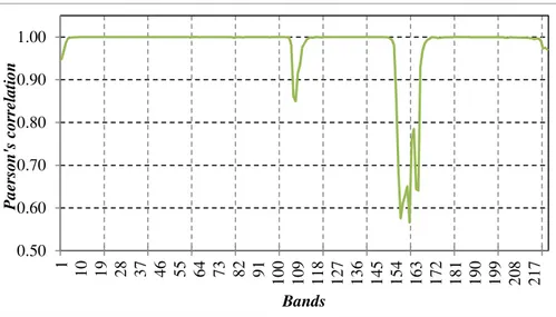
the same materials. Thus, adjacent pixel values are effectively correlated in the space (intra-band correlation). Similarly, it is observable that consecutive spectral bands show a high correlation (inter-band correlation). In Figure 2.8, a graph of the Pearson’s correlation among all the bands of an AVIRIS hyperspectral image is shown. In detail, on the Y-axis the value assumed by the Pearson’s correlation, obtained by considering the i-th and the (𝑖 − 1)-th bands (the bands are reported on the 𝑋-axis), is reported.
It is noticeable that the correlation assumes high values (around 0.999) in most of the cases. Only a subset of bands, which are affected by noise, present low correlation values.
Figure 2.8: The trend of the Pearson’s correlation among the spectral band of
an AVIRIS datacube (the “Lunar Lake scene 03” image).
0.50 0.60 0.70 0.80 0.90 1.00 1 1 0 1 9 2 8 3 7 4 6 5 5 6 4 7 3 8 2 9 1 1 0 0 1 0 9 1 1 8 1 2 7 1 3 6 1 4 5 1 5 4 1 6 3 1 7 2 1 8 1 1 9 0 1 9 9 2 0 8 2 1 7 P a e r s o n 's c o r r e la ti o n Bands
27
2.5.
5-D Functional Magnetic Resonance Imaging
(fMRI)
Over recent years, many methods have been proposed with the main objective being to investigate the functioning of the human brain. Mainly, the research activities have focused on specific brain regional and functional features. One of the main objectives is to identify and, consequently, evaluate the distribution of the neural activities in the brain as a whole at a given moment.
Functional Magnetic Resonance Imaging (functional MRI or fMRI) allows to
measure the hemodynamic response (change in blood flow), related to neural activity in the brain. In detail, through fMRI techniques, it is possible to observe the neuronal activities, characterized by neuroactivation task, which need metabolic oxygen support. It is important to point out that a fMRI scanner is a type of specialized MRI scanner.
The fMRI technique is a fundamental tool for assessing the neurological status and neurosurgical risk of a patient and, through its capabilities, the brain anatomical imaging is extended. Furthermore, by analyzing these data, it is possible to determine the regions of the brain that are activated by a particular task. In particular, a fMRI scanner is able to map different structures and specific functions of the human brain.
Different clinical applications use fMRI for the localization of brain functions, the searching of markers of pathological states, etc.. In particular, fMRI techniques are helpful in identifying preclinical expressions of diseases and developing new treatments for them [7].
28
Consequently, a fMRI scanner produces a dataset, which is composed of a collection of 3-D data volumes (T dimension). Each volume is substantially a collection (on the Z dimension) of bi-dimensional images (X and Y dimensions). In general, multiple trials of observation are performed (R dimension), in order to improve the accuracy of the examination. It is evident that such data can be viewed a multidimensional data (where 𝑁 can be equal to 4 or equal to 5).
30
Chapter
Chapter
Chapter
Chapter –
–
–
–
3
3
3
3
Low-Complexity Lossless Compression of 3-D Medical Images
Highlights of the chapter
3.1. Lossless and Low-Complexity Compression
of 3-D Medical Images
3.1.1. and 3.1.2. The Predictors 3.1.3. Error Modeling and Coding 3.1.4. Experimental Results
p. 32
3.2. Parallel Low-Complexity Lossless
Compression of 3-D Medical Images
3.2.1. Review of the OpenCL Framework 3.2.2. Description of the Parallel MILC 3.2.3. The Host Program
3.2.4. The OpenCL Kernel 3.2.5. Experimental Results
31
In this chapter, we describe a predictive-based approach for lossless compression of 3-D medical images (such as 3-D MR, 3-D CT, etc.). In detail, our method is characterized by the low usage of computational resources and the parsimonious usage of memory. Furthermore, it is easily implementable and provides a good trade-off between computational complexity and compression performances.
By considering the medical and medical-related contexts, in which the time could be a critical parameter, we focus on the improvement of the execution time of our approach. In particular, we exploit the capability of the parallel computing, in order to design a parallelized version of the compression strategy of the proposed method.
32
3.1.
Lossless and Low-Complexity Compression of
3-D Medical Images
In different medicine and healthcare scenarios, it could be relevant to consider the efficiency of an algorithm in terms of execution time, which is involved in the analysis and/or processing of medical data. In particular, this aspect might be fundamental in many medical applications. Generally, algorithms with a low usage of computational resources are efficient in terms of execution time. In the case of lossless compression algorithms, it is important to take into account the trade-off between the compression performances and the execution time/computational complexity.
Considering the delicate medical circumstances, during the design phases of a compression scheme, it is essential to take into account and examine, which strategy, between lossless and lossy, could be employed. In particular, the lossy compression strategies are used only in a few cases, while lossless compression techniques are generally preferred. In fact, starting from the coded data, it is possible to get back the original data through lossless strategies.
In this section, we describe a lossless compression technique for 3-D medical images, we referred to it as Medical Images Lossless Compression algorithm (MILC). In detail, MILC uses limited resources in terms of computational power and memory.
33
Figure 3.1: The MILC diagram block (adapted from [20]).
Figure 3.1 shows the MILC diagram block, with our approach being based on the predictive model and using two predictors:
• 2-D Linearized Median Predictor (2D-LMP);
• 3-D Distances-based Linearized Median Predictor (3D-DLMP).
In particular, MILC processes each sample, 𝑥(0), of the input 3-D medical image. It should be noted that the 2D-LMP predictor (described in Section 3.1.1) is used only for the first slice, which has no previous reference slices. Thus, the 2D-LMP exploits only the intra-slice correlation.
On the other hand, the 3D-DLMP predictor (explained in Section 3.1.2) is used for all the samples of all the slices (except for the first). It is important to point out that both the intra-slice and inter-slice correlations are exploited by the 3D-DLMP.
Finally, once a sample is predicted, the related prediction error is computed by calculating the difference between the sample, 𝑥(0), and the predicted
34
sample, 𝑥̂(0). Then, the prediction error is modeled and coded, as explained in Section 3.1.3.
3.1.1.
The 2-D Linearized Median Predictor (2D-LMP)
The 2D-LMP predictive structure uses a prediction context composed only by samples, which belong to the same slice of the current sample, 𝑥(0).
In particular, three neighboring samples of 𝑥(0) are used, namely, 𝑥(1), 𝑥(2) and 𝑥(3). Figure 3.2 shows a graphical example of the prediction context used by the 2D-LMP. It should be noted that the light blue samples are already processed and coded.
It is important to point out that the prediction of 𝑥(0) is obtained by means of the equation (3.1).
𝑥̂(0) = 2(𝑥(1)+ 𝑥(2))
3 − 𝑥
(3)
3 (3.1)
Figure 3.2: A graphical example of the prediction context used by
35
In detail, this predictive structure is derived from the well-known predictive structure of the Median Predictor [24, 38], used in the JPEG-LS algorithm.
𝑥̂(0) = ⎩ { ⎨ { ⎧ min(𝑥(1), 𝑥(2)) max(𝑥(1), 𝑥(2)) 𝑥(1)+ 𝑥(2)− 𝑥(3) 𝑖𝑓 𝑥(3) ≥ max(𝑥(1), 𝑥(2)) 𝑖𝑓 𝑥(3) ≤ min(𝑥(1), 𝑥(2)) 𝑜𝑡ℎ𝑒𝑟𝑤𝑖𝑠𝑒 (3.2)
As may be observed from the equation (3.2), which reports the predictive structure of the Median Predictor, one of three possible options is used by the latter predictor for the computing of the prediction. The capability of the 2D-LMP predictor is to combine all of these three options, as explained by equation (3.3). 𝑥̂(0) = 13(max(𝑥(1), 𝑥(2)) + min(𝑥(1), 𝑥(2)) + (𝑥(1)+ 𝑥(2)− 𝑥(3)) = = 13((𝑥(1)+ 𝑥(2)) + (𝑥(1)+ 𝑥(2) − 𝑥(3))) = = 13(2 (𝑥(1)+ 𝑥(2)) − 𝑥(3)) = = 2(𝑥(1)3+ 𝑥(2))− 𝑥3(3) (3.3)
It is noticeable that the third line of the equation (3.3) is obtained because min(𝑥(1), 𝑥(2)) + max(𝑥(1), 𝑥(2)) = 𝑥(1) + 𝑥(2).
36
3.1.2.
The 3-D Distances-based Linearized Median
Predictor (3D-DLMP)
The 3D-DLMP predictor exploits the inter-slice and intra-slice correlations. In particular, the used prediction context is composed by neighbors of the current sample, 𝑥(0), in the current slice as well as the previous slice. In detail, three adjacent samples of the current sample in the same slice (i.e., 𝑥(1), 𝑥(2) and 𝑥(3)) and three adjacent samples in the previous slice (i.e., 𝑥(1)(−1), 𝑥(2)(−1)
and 𝑥(3)(−1)), compose the prediction context. Moreover, also the sample, with the same spatial coordinates of the current sample of the previous slice (𝑥(0)(−1)), is used.
Figure 3.3 shows a graphical representation of the prediction context, used by the 3D-DLMP. It is important to note that the light blue samples are already coded.
Figure 3.3: A graphical example of the prediction context used by
37
Basically, three main steps are needed to implement the 3D-DLMP: 1) Computing of the distances;
2) Computing of a sort of average distance; 3) Computing of the prediction.
In step (1), the distances between the samples of the current slice and the samples of the previous slice are computed, by means of the equations (3.4), (3.5) and (3.6).
𝛿𝑥(1) = 𝑥(1)− 𝑥(1)(−1) (3.4)
𝛿𝑥(2) = 𝑥(2)− 𝑥(2)(−1) (3.5)
𝛿𝑥(3) = 𝑥(3)− 𝑥(3)(−1) (3.6)
These differences are used in step (2), in which a sort of “average distance”, we denoted as 𝛿, is obtained. The equation (3.7) defines how 𝛿 is computed.
𝛿 = 2(𝛿𝑥(1) + 𝛿𝑥(2))
3 − 𝛿𝑥
(3)
3 (3.7)
In step (3), the prediction of the current sample is performed, as explained in the equation (3.8). In detail, the above computed distance, 𝛿, is added to the sample 𝑥(0)(−1).
𝑥̂(0) = 𝑥(0)(−1) + 𝛿 (3.8)
It is easy to note that the 3D-DLMP predictor is based on the 2D-LMP predictive structure, which is described in the previous subsection. Moreover, the 3D-DLMP predictor can be further optimized, in terms of the number of operations related to the prediction of a sample.
38
In equation (3.9), we report the optimized predictive structure, in which only 1 division and 7 additions/subtractions are involved, by also taking into account the computing of 𝛿𝑥(1)𝑥(2).
𝑥(0) = 𝑥(0)(−1) + 𝛿𝑥(1)𝑥(2) + 𝛿𝑥(1)𝑥(2) − 𝛿𝑥(3)
3 (3.9)
In particular, the computation of 𝛿𝑥(1)𝑥(2) is performed by means of the
equation (3.10).
𝛿𝑥(1)𝑥(2) = 𝛿𝑥(1) + 𝛿𝑥(2) (3.10)
3.1.3.
Error Modeling and Coding
The prediction error related to the current sample, 𝑥(0), is obtained by means of the equation (3.11).
𝑒𝑥(0) = ⌊𝑥(0) − 𝑥̂(0)⌋ (3.11)
In detail, the prediction error is first mapped, by using the mapping function of the equation (3.12), and then the mapped error is encoded through the
Prediction by Partial Matching with Information Inheritance (PPMII or
PPMd) encoding scheme [29].
𝑚(𝑒𝑥(0)) = { 2 × |𝑒𝑥(0)| 𝑖𝑓 𝑒𝑥(0) > 0
39
It is important to remark that the PPMd algorithm improves the efficiency of PPM [30]. In particular, its complexity is comparable with other compression schemes, for example LZ77 [31], LZ78 [32], BWT Transform [33].
It is important to emphasize that all the prediction residuals constitute a
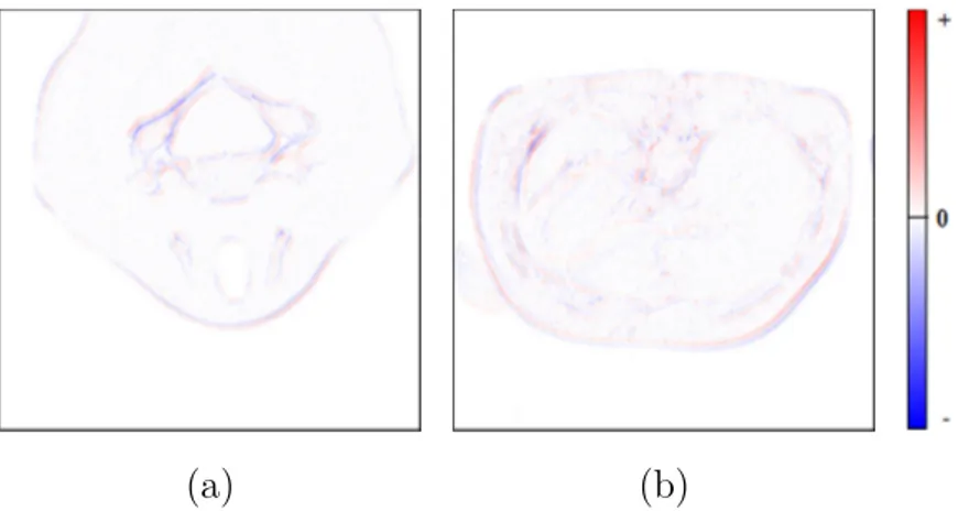
residual image [55]. Figures 3.4.a and 3.4.b show two graphical examples of
residual images in false-color, of a slice of a CT image (“CT_carotid”) and of a MR image (“MR_liver_t2e1”), respectively. Such residual images are obtained by using the 3D-DLMP predictive structure. The positive errors are represented through a gradient of color, which varies from white to red, and the negative errors are represented through a gradient, which varies from white to blue. It is important to point out that the color intensity proportionally grows with respect to the value of the prediction error.
In Figure 3.5, we graphically report the distribution of prediction errors related to a slice of a MR image (the “MR_liver_t1” image). It should be noted that such distribution follows a skewed Laplacian-like distribution, centered on zero. In general, we obtain similar distributions for all the slices of a 3-D medical image, by using our predictive structures. In literature, Laplacian-like distributions of prediction errors are efficiently modeled and coded [18].
40
(a) (b)
Figure 3.4: A false-color residual image of a slice of a CT image (a)
and of a MR image (b) (from [20]).
Figure 3.5: The prediction error distribution of a slice
of a MR image (from [20])
3.1.4.
Experimental Results
This section focusses on the experimental results achieved by using our approach on the dataset described in Appendix A.1, which is composed of four 3-D CT images and four 3-D MR images. It is important to point out that we
41
experimentally performed our approach by using two different orders (i.e., 2 and 4) for the coding of the prediction errors through the PPMd algorithm. In detail, Table 3.1 reports the experimental results, in terms of BPS, for each one of the CT images. In particular, the first column reports the images, while the second and third columns report the results by using the order equal to 2 and the order equal to 4 for the coding of the prediction errors, respectively. Analogously to Table 3.1, in Table 3.2 we report the achieved experimental results on the MR images.
It is easy to note that our approach obtains better results when the order is set to 4. However, the computational complexity of PPMd is affected by increasing the order.
In addition, we analyzed the coding of prediction errors in terms of required memory through the PPMd scheme, for both the used orders.
Table 3.1: Experimental results achieved on the CT images. Images MILC (PPMd o = 𝟐) MILC (PPMd o = 𝟒) CT_skull 2.0683 2.0306 CT_wrist 1.0776 1.0666 CT_carotid 1.4087 1.3584 CT_Aperts 0.8473 0.8190 Average 1.3505 1.3187
42
Table 3.2: Experimental results achieved on the MR images. Images MILC (PPMd o = 𝟐) MILC (PPMd o = 𝟒) MR_liver_t1 2.1839 2.1968 MR_liver_t2e1 1.7749 1.7590 MR_sag_head 2.1201 2.0975 MR_ped_chest 1.6612 1.6556 Average 1.9350 1.9272
Table 3.3: Memory usage for the coding of prediction errors
on the CT images. Method /
Images CT_skull CT_wrist CT_carotid CT_Aperts Average
PPMd
(order = 4) 9.90 0.70 2.50 1.40 3.63
PPMd
(order = 2) 0.40 0.10 0.30 0.10 0.23
Table 3.4: Memory usage for the coding of prediction errors
on the MR images. Method /
Images MR_liver_t1 MR_liver_t2e1 MR_sag_head MR_ped_chest Average
PPMd
(order = 4) 1.50 3.60 4.10 0.70 2.48
PPMd
(order = 2) 0.10 0.20 0.30 0.10 0.18
In Tables 3.3 and 3.4, we report the used memory (in terms of Megabytes), related to the coding of the errors. In particular, the first column indicates the
43
used order for the PPMd scheme, the columns from the second to the fifth indicate the images and the last column indicates the average.
In Figures 3.6 and 3.7, we graphically represent the information contained in Table 3.3 and Table 3.4, respectively.
Figure 3.6: A graphical representation of Table 3.3.
Figure 3.7: A graphical representation of Table 3.4.
0.00 2.00 4.00 6.00 8.00 10.00 12.00
CT_skull CT_wrist CT_carotid CT_Aperts
M B CT Images MILC (PPMd o = 4) MILC (PPMd o = 2) 0.00 0.50 1.00 1.50 2.00 2.50 3.00 3.50 4.00 4.50
CT_skull CT_wrist CT_carotid CT_Aperts
M
B
MR Images
MILC (PPMd o = 4) MILC (PPMd o = 2)
44
The figures show how by setting the order equal to 4 for the PPMd scheme, MILC uses 16 times (CT images) and 14 times (MR images) more memory with respect to the case in which the order is set to 2.
3.1.5.
Discussion of Results
We compare the results achieved by using the MILC algorithm with respect to other currently used approaches.
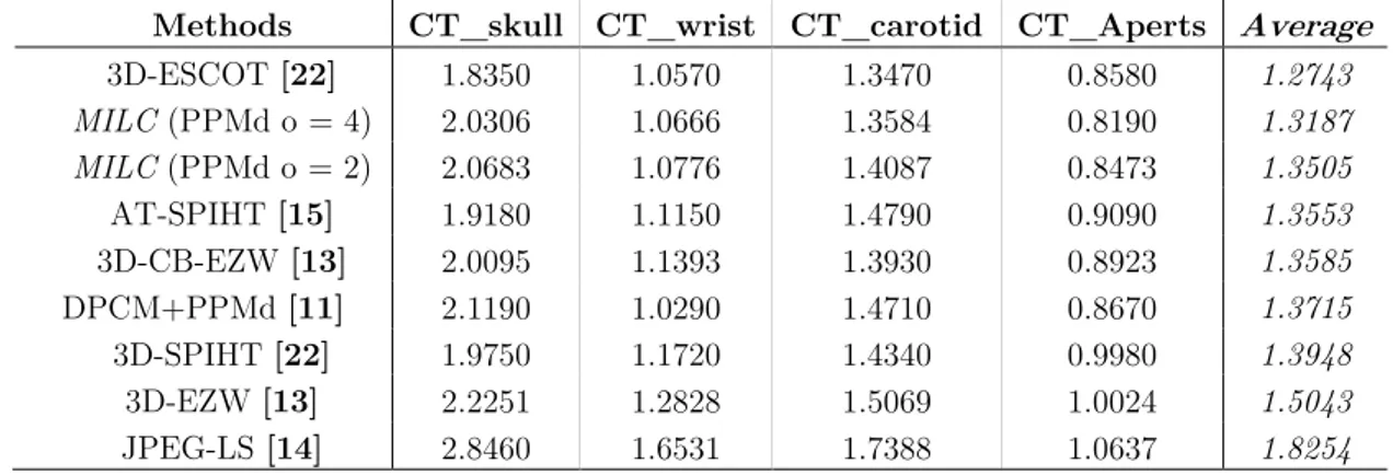
In Table 3.5, we report the results in terms of bits-per-sample (BPS), for each one of the CT images (the columns from the second to the fifth), obtained by using different methods (first column) and, in the last column, the average of the results related to a method is reported.
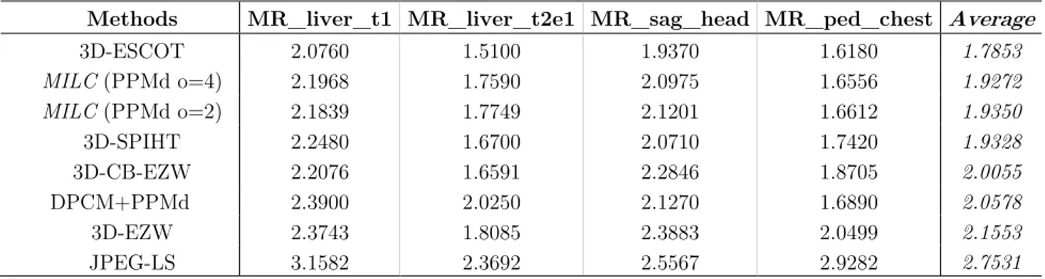
Similarly to Table 3.5, in Table 3.6 we report the achieved results for the MR images.
Table 3.5: Memory usage for the coding of prediction errors
on the MR images.
Methods CT_skull CT_wrist CT_carotid CT_Aperts Average
3D-ESCOT [22] 1.8350 1.0570 1.3470 0.8580 1.2743 MILC (PPMd o = 4) 2.0306 1.0666 1.3584 0.8190 1.3187 MILC (PPMd o = 2) 2.0683 1.0776 1.4087 0.8473 1.3505 AT-SPIHT [15] 1.9180 1.1150 1.4790 0.9090 1.3553 3D-CB-EZW [13] 2.0095 1.1393 1.3930 0.8923 1.3585 DPCM+PPMd [11] 2.1190 1.0290 1.4710 0.8670 1.3715 3D-SPIHT [22] 1.9750 1.1720 1.4340 0.9980 1.3948 3D-EZW [13] 2.2251 1.2828 1.5069 1.0024 1.5043 JPEG-LS [14] 2.8460 1.6531 1.7388 1.0637 1.8254
45
Table 3.6: Memory usage for the coding of prediction errors
on the MR images.
Methods MR_liver_t1 MR_liver_t2e1 MR_sag_head MR_ped_chest Average
3D-ESCOT 2.0760 1.5100 1.9370 1.6180 1.7853 MILC (PPMd o=4) 2.1968 1.7590 2.0975 1.6556 1.9272 MILC (PPMd o=2) 2.1839 1.7749 2.1201 1.6612 1.9350 3D-SPIHT 2.2480 1.6700 2.0710 1.7420 1.9328 3D-CB-EZW 2.2076 1.6591 2.2846 1.8705 2.0055 DPCM+PPMd 2.3900 2.0250 2.1270 1.6890 2.0578 3D-EZW 2.3743 1.8085 2.3883 2.0499 2.1553 JPEG-LS 3.1582 2.3692 2.5567 2.9282 2.7531
As can be observed from the tables, the results achieved, on average, for the 3-D CT images are slightly worse than the 33-D-ESCOT approach, which is the most performing schema. In detail, our approach outperforms 3D-ESCOT only in the case of the “CT_Aperts” image. Regarding the case of the 3-D MR images, the results achieved by the MILC algorithm, are significantly worse with respect to the 3D-ESCOT algorithm.
On the other hand, the MILC approach presents different advantages related to the trade-off between the computational complexity and the compression performances. In particular, the possibility to easily implement our approach and the low resources usage, with our approach being preferable in various scenarios, even in the case of hardware restrictions.
46
3.2.
Parallel Low-Complexity Lossless Compression
of 3-D Medical Images
In this section, we focus on the review of a novel design and implementation for the MILC compression algorithm, which is denoted as “Parallel MILC”
[15]. In particular, Parallel MILC is able to exploit the features and
capabilities of the parallel computing paradigm. It is important to consider that our approach can be executed on several heterogeneous devices, which support the OpenCL framework. Currently, there are many types of devices that support the OpenCL framework, for example Central Processing Units (CPUs), Graphic Processing Units (GPUs), Field Programmable Gate Arrays (FPGAs), etc.. The main aim of Parallel MILC is to improve the execution time of the compression algorithm.
In detail, our objective is the redesigning of the MILC compression strategy, according to the OpenCL framework. The key points of this framework are briefly reviewed in the following subsection.
3.2.1.
Review of the OpenCL Framework
The Open Computing Language (OpenCL) allows to design parallelized applications. An Open CL-based application can be executed across heterogeneous platforms, i.e., CPUs, GPUs, FPGAs as well as many others. It is important to point out that OpenCL supports both task-based and data-based parallelism.
47
Regarding the OpenCL platform model, it is easy to note that only a single
Host entity is included in the model. In detail, as shown in Figure 3.8, the Host
is connected to one or more device(s). The devices connected to the Host, need to support the OpenCL framework, and are denoted as OpenCL devices.
In this case, the Host serves as a sort of “connection point” between the OpenCL devices and the external environment (i.e. I/O, interactions with the end-user, etc.). On the other hand, an OpenCL device is able to execute a stream of instructions or a function (denoted as the kernel).
By focusing on the logical architecture of an OpenCL device (graphically represented in Figure 3.9), it is easy to find out that such device can be composed by one or more Compute Units (CUs). Furthermore, a CU can be composed of different Processing Elements (PEs).
Figure 3.8: Graphical representation of the OpenCL platform model.
Generally, an application based on the OpenCL framework is characterized by two main components:
48
• The host program; • One or more kernels.
The host program has to be executed on the Host entity, while the kernel(s) have to be executed on the OpenCL device(s). In detail, the OpenCL standard has no explicit definitions on how a host program works [39]. Nevertheless, the interactions with the OpenCL objects are well defined [39]. While, the kernel is substantially a sort of function, which is charge of implementing all (or a significant portion) of the application logic of a program. In particular, through the kernel is possible to perform the logical work of such programs [39, 40]. Two main types of kernels are defined by the OpenCL framework, namely,
OpenCL kernels and native kernels. An OpenCL kernel is characterized by the
possibility to program it through the embedded C-based programming language (i.e. the OpenCL C language). Furthermore, it can be compiled through an OpenCL compiler and executed over any OpenCL device. Regarding a native kernel, it can be composed of one or more external functions, which can be accessed by OpenCL through a specific function pointer [39].
It is important to take into account another fundamental aspect of the OpenCL framework, relating to the manner in which a kernel is executed. Considering a basic example, in which a host program has been defined a kernel. The host program is able to invoke, by using a proper command, the execution of the kernel on one or more OpenCL devices.
In particular, once an OpenCL device has received such a command, the relative “runtime environment” enables it to create an integer index space,
49
which is denoted as NDRange [39]. It is important to emphasize that an instance of NDRange characterizes a 𝑁-dimensional index space. The current version of the OpenCL framework (1.2) allows to create an 𝑁-dimensional instance of NDRange, with 𝑁 ∈ {1, 2, 3}. Thus, the simplest type of instance of NDRange can describe a 1-dimensional integer space (𝑁 = 1). In this case, the instance of NDRange is defined as a sort of linear array of a given size.
Subsequently, in each “point” of the instance, a kernel is instantiated. It should be noted that a kernel under execution is denoted as “work-item”, and can be addressed through its 𝑁 global identifiers (global IDs), where 𝑁 is the number of the dimensions of the instance. For example, in a bi-dimensional NDRange (where 𝑁 = 2), it is possible to address a work-item through two global IDs (each one related to a dimension).
The work-items can be organized into groups (work-groups), which can be identified by their group identifier (work-group ID).
Another main point of OpenCL is the memory model. Substantially, two main types of objects are defined by the framework, namely, the buffer and the
image objects. Basically, a buffer object can be viewed as a portion of memory
provided by the kernel, which the programmer can use as wanted (i.e. to store data structure, arrays, matrices, etc.). While an image object can be used for the management of images.
50
Figure 3.9: Graphical representation of the logical architecture of an OpenCL
device.
Furthermore, five memory regions are defined by the memory model and can be used in OpenCL-based applications:
• Host Memory; • Private Memory; • Local Memory; • Global Memory; • Constant Memory.
In particular, the Host Memory is a memory region accessible and modifiable only by the host. Whereas, the other regions are accessed by the OpenCL devices. The Private and Local Memory can be only accessed/modified respectively by a work-item and a work-group. Furthermore, the Global Memory is accessible/modifiable by all the work-items. Analogously to the
51
Global Memory, the Constant Memory is accessible by all the work-items with the limitation that this region is not modifiable.
3.2.2.
Description of the Parallel MILC
As discussed in Section 3.1, the MILC algorithm processes each sample of the input 3-D medical image, in the raster-scan order. In particular, each sample is predicted and its related prediction error is mapped and sent to the PPMd encoding scheme. On the other hand, from the coded stream the MILC decompression algorithm is able to process the next prediction error (after it has been performed both the PPMd decoding and the inverse mapping phases). By using the obtained prediction error, the inverse prediction is performed and the reconstructed sample is then written to the decoded stream.
Thus, the final decoded stream will be equal to the original uncompressed image. It is worth noting that the order in which the prediction errors are stored is essential, because is the same as the original uncompressed image.
The basic idea behind the Parallel MILC compression strategy is related to the assumption that each sample can be “independently predicted”, provided that the whole 3-D medical image has been acquired. In such scenario, it is noticeable that several samples are processed at the same time, in different manner with respect to the MILC. Thus, it is not possible an “a priori” estimation in relation to the order, in which the prediction errors will be generated. However, by using some information related to the data format (i.e.
52
about the storing order of the samples) of the input 3-D medical image, such an issue can be solved.
In detail, through the coordinates of a sample, it is possible to store its related prediction error into a specific position (𝑝) of a temporary buffer. This buffer maintains the residual image. Once the prediction of all the samples is computed, the whole temporary buffer is sent to the PPMd scheme.
It is important to emphasize that MILC does not need any information about the data format and does not require any buffer for the maintaining of the residual image. The latter are the main differences and drawbacks of Parallel MILC with respect to MILC.
Since it is generally easy to identify the data format of the input 3-D medical image, and, consequently, the processing order of the samples, the first one should not always be considered a drawback. It is important to remark that in medical and medical-related environments in which time may be a “critical” parameter, the effective speedup obtained in the Parallel MILC execution performance could justify such issues.
An important aspect related to the operation logic of the Parallel MILC decompression algorithm is that it is the same as the one used by MILC. Thus, it is possible to encode a medical image transparently, by using MILC or Parallel MILC. Thus, the coded stream can be decoded always in the same way.
It is important to note that Parallel MILC is an OpenCL application, therefore, it is characterized by the host program and an OpenCL kernel.