Feynman-diagrams approach to the quantum Rabi model for ultrastrong cavity QED: Stimulated emission and reabsorption of virtual particles dressing a physical excitation

This content has been downloaded from IOPscience. Please scroll down to see the full text.

Download details:

IP Address: 134.160.214.34

This content was downloaded on 17/05/2017 at 03:20

Please note that terms and conditions apply.

Feynman-diagrams approach to the quantum Rabi model for ultrastrong cavity QED:

stimulated emission and reabsorption of virtual particles dressing a physical excitation

View the table of contents for this issue, or go to the journal homepage for more 2017 New J. Phys. 19 053010

New J. Phys. 19(2017) 053010 https://doi.org/10.1088/1367-2630/aa6cd7

PAPER

Feynman-diagrams approach to the quantum Rabi model for

ultrastrong cavity QED: stimulated emission and reabsorption of

virtual particles dressing a physical excitation

Omar Di Stefano1,2,5_{, Roberto Stassi}2_{, Luigi Garziano}3_{, Anton Frisk Kockum}2_{, Salvatore Savasta}1,2_and Franco Nori2,4

1 _{MIFT—Dipartimento di Scienze Matematiche e Informatiche Scienze Fisiche e Scienze della Terra, Università di Messina, I-98166}

Messina, Italy

2 _{CEMS, RIKEN, Saitama 351-0198, Japan}

3 _{University of Southampton, Southampton, SO17 1BJ, United Kingdom}

4 _{Physics Department, The University of Michigan, Ann Arbor, Michigan 48109-1040, United States of America} 5 _{Author to whom any correspondence should be addressed.}

E-mail:email: odistefano@unime.it

Keywords: ultrastrong-coupling regime, virtual particles, Feynman diagrams, cavity-QED, quantum vacuum_{fluctuations, three-level} quantum system

Abstract

In quantum

field theory, bare particles are dressed by a cloud of virtual particles to form physical

particles. The virtual particles affect properties such as the mass and charge of the physical particles,

and it is only these modified properties that can be measured in experiments, not the properties of the

bare particles. The influence of virtual particles is prominent in the ultrastrong-coupling regime of

cavity quantum electrodynamics

(QED), which has recently been realised in several condensed-matter

systems. In some of these systems, the effective interaction between atom-like transitions and the

cavity photons can be switched on or off by external control pulses. This offers unprecedented

possibilities for exploring quantum vacuum

fluctuations and the relation between physical and bare

particles. We consider a single three-level quantum system coupled to an optical resonator. Here we

show that, by applying external electromagnetic pulses of suitable amplitude and frequency, each

virtual photon dressing a physical excitation in cavity-QED systems can be converted into a physical

observable photon, and back again. In this way, the hidden relationship between the bare and the

physical excitations can be unravelled and becomes experimentally testable. The conversion between

virtual and physical photons can be clearly pictured using Feynman diagrams with cut loops.

1. Introduction

In quantumfield theory (QFT), the creation and annihilation operators in the Lagrangian describe the creation and destruction of bare particles which, however, can not be directly observed in experiments(see, e.g., [1,2]).

Bare particles, due to the interaction terms in the Lagrangian, are actually dressed by virtual particles and become real physical particles which can be detected. The interaction modifies the properties of the particles, e.g., giving rise to the Lamb shift of electronic energy levels[3,4] and affecting the charge, mass, and magnetic moment of

the electron[1,5,6]. The predictions of the theory must be expressed in terms of the properties of the physical

particles, not of the non-interacting(or bare) particles [1,2]. The relations between the bare and the physical

particles are unobservable.

The influence of virtual particles features prominently in the ultrastrong coupling (USC) regime of cavity quantum electrodynamics(QED) [7,8]. In cavity QED [9], the interaction between light confined in a reflective

cavity and natural or artificial atoms is studied in conditions where the quantum nature of light is important. The system enters the USC regime when the light–matter coupling rate becomes an appreciable fraction of the unperturbed resonance frequencies of the photons and the atom. In this regime, the routinely-invoked rotating OPEN ACCESS

RECEIVED 30 January 2017 REVISED 27 March 2017 ACCEPTED FOR PUBLICATION 12 April 2017 PUBLISHED 16 May 2017

Original content from this work may be used under the terms of theCreative Commons Attribution 3.0 licence.

Any further distribution of this work must maintain attribution to the author(s) and the title of the work, journal citation and DOI.

wave approximation(RWA) is no longer applicable and the counter-rotating terms in the light–matter

interaction significantly change the standard cavity QED scenario [7,8,10–22]. For example, very recently it has

been shown that, in the USC regime, a single photon can excite two or more atoms[21]. This effect can occur

because the atom-cavity system can essentially borrow the needed second virtual photon from the quantum vacuum. In the past few years, the USC regime has been reached experimentally in a variety of solid-state systems and spectral ranges[23–37].

The need to distinguish between virtual and physical particles in the USC regime of cavity QED is

exemplified by the fact that the correct description of the output photon flux from the cavity, as well as of higher-order Glauber normal-higher-order correlation functions, requires a proper generalisation of input–output theory [15,38]. Due to the contribution from counter-rotating terms in the interaction Hamiltonian, the ground state

ñ

∣E0 of the system contains afinite number of photons [39], i.e.,

á_E ∣ ˆ ˆ ∣_{a a E}† ñ ¹_0,

0 0

where ˆa and_aˆ†_{are the annihilation and creation operators for the cavity mode. However, the ground state can}

not emit energy, so the output photonflux can not be proportional to á_{a a , as in standard input}ˆ ˆ† ñ _{–output theory.}

Instead, it has been shown[15,40] that the cavity output (which can be detected by a photo-absorber) is

proportional toáx xˆ ˆ- +ñ, wherexˆ+is the positive frequency component of the quadrature operator_xˆ= +_aˆ _aˆ†

and_xˆ-=( ˆ )_x+†_{. The result}

á_{E ∣ ˆ ˆ ∣x x}- + _E ñ =₀

0 0

demonstrates that the photons that contribute to the ground state are not observable physical particles. An analogous situation arises when the photons are coupled to collective matter excitations described by bosonic fields [41]. It can also be shown that the (physical) system excitations are enriched by unobservable virtual

particles. For instance, thefirst excited state, corresponding to a single physical particle, may contain

contributions from an odd number of excitations. All these unobservable contributions, however, are significant only in the USC regime, not at weaker coupling strengths. An interesting feature of these condensed-matter systems is that the effective interaction between atom-like transitions and the cavityfield can be switched on and off by applying external drives. This offers the opportunity to convert the virtual excitations into real particles which can then be detected. Both spontaneous[7] and optically [42] or electrically [43] stimulated conversion of

virtual photons from the ground state of a cavity QED system in the USC regime have recently been analysed. Also, virtual photon pairs are converted into real ones in the dynamical Casimir effect(DCE) [44], which has

been analysed[45–47] and experimentally demonstrated [48] in circuit QED. Potentially, a proper modulation

of an effective mirror(i.e., an oscillating boundary condition) in a DCE setup could also allow for absorption of photon pairs[49].

Here we show how to convert various numbers of virtual photons into real ones and back, both for the dressed vacuum state and for a dressed excited state, in a three-level system with one transition ultrastrongly coupled to an optical resonator. We also show that the corresponding Feynman diagrams can be obtained by cutting the loop diagrams describing the energy correction of a physical excitation. Specifically, conversion of virtual photons dressing a physical excitation into real ones is described by thefirst half of cut loop-diagrams (photon emission). Similarly, the conversion of real photons back into virtual ones bound to a physical excitation corresponds to the second half(photon absorption). Moreover, the proposed scheme does not require the ultrafast modulation of boundary conditions and it can give rise to a conversion probability close to one.

2. Results

2.1. The quantum Rabi model

The simplest cavity-QED model beyond the RWA is the quantum Rabi model[50,51]. The Hamiltonian is

( = 1)_Hˆ_R=_Hˆ₀+_Vˆ_{, whereH}ˆ =w _{a aˆ ˆ}† +w _{∣e e}ñá +_∣ w _{∣g g}ñá _∣

e g

0 c is the bare Hamiltonian in the absence of

interaction. Here, ˆa and_aˆ†_{are the photon destruction and creation operators for the cavity mode with}

resonance frequency w ;c ∣gñand∣eñare the ground and excited atomic states, respectively, andwe g( )are the

corresponding energy eigenvalues. The interaction Hamiltonian is

s

= W +

ˆ _{( ˆ}† ˆ) ˆ ( )

V R a a x, 1

where WRis the coupling strength and sˆx=sˆ++sˆ-= ñá + ñá∣e g∣ ∣g e∣. When wc »weg ºwe-wg, the interaction Hamiltonian can be separated into a resonant and a non-resonant part:Vˆ =Vˆr+Vˆnr, where

s s

= W -+ +

ˆ _{( ˆ ˆ}† _{ˆ ˆ )}

Vr R a a , andVˆnr= WR( ˆ ˆa†s++aˆ ˆ )s-. The counter-rotating terms do not conserve the number of

excitations. They can be neglected whenWR (wc+weg)1. The interaction Hamiltonian has a structure which is very similar to that of the QED interaction potential, although it is less complicated. The quantum Rabi

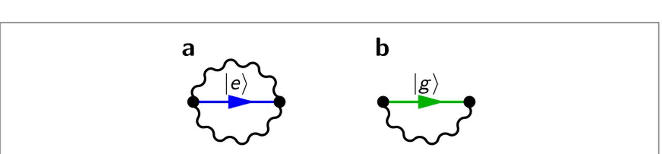
model can be viewed as a very simple QED system, where there is only a single photon mode and a two-state electron. As a consequence, we would expect that Feynman diagrams for the Rabi Hamiltonian will be a simplified version of QED diagrams. One such diagram, for the counter-rotating transition∣g, 0ñ ∣e, 1ñ(the second entry in the ket denotes the photon number), is shown in figure1(a).

However, some care must be taken when drawing diagrams for processes involving more than one photon in the same mode[52], which occur in cavity QED. Stimulated emission [53], the mechanism behind laser action, is

one such process. It is a one-photon process∣e n, ñ ∣g n, + ñ1 , where the n photons in the initial state stimulate the downward transition of the atom, affecting the transition rate which becomes proportional to

+

n 1. This factor must be included in the rules for the diagrams in order for calculations to be correct. An example of a diagram showing the stimulated-emission process∣e, 1ñ ∣g, 2 is presented inñ figure1(b). A

more detailed discussion about diagrams for stimulated emission can be found in appendixA.

2.2. Bare versus physical excitations

Owing to the presence of ˆVnrin the Rabi Hamiltonian, the operator describing the total number of excitations,

= + ñá

ˆ _{ˆ ˆ}† _{∣ ∣}

N a a e e , does not commute withHˆRand as a consequence the eigenstates ofHˆRdo not have a definite

number of excitations[39]. When ˆVnrcan be neglected, the Hamiltonian becomes block-diagonal and easy to

diagonalize(this is the Jaynes–Cummings (JC) model [54]). The resulting eigenstates can be labelled according

to their definite number of excitations n. The ground state (zero excitations) is simply  ñ =∣ 0 ∣g, 0ñ, and the 

n 1 excitation states  ñ∣ n , obtained by diagonalization of 2×2 subspaces, can be written as

+ñ = ñ + - ñ -ñ = - ñ + - ñ

∣ _n n∣g n, n∣e n, 1 ∣ n n∣g n, n∣e n, 1 , ( )2

where nand nare amplitudes determined by WRand the detuning wc -weg. The eigenstates∣Eiñof the full Rabi Hamiltonian, however, are expressed as a superposition of bare states with varying numbers of bare excitations(see, e.g., [40]):

å

where the coefficients cg ki, andde ki, are determined by WR,wcandweg. WhenW R w wc, eg, the Rabi eigenstates reduce to the JC ones. Note that whileNˆ is not conserved with the Rabi Hamiltonian, the parity(even or odd number of excitations) still is [10,55–57].

The mean photon number for the system in its ground state is

å

á_E ∣ ˆ ˆ ∣_{a a E}† ñ = _{k c}(∣ ∣ +∣_d ∣ )_. ( )₄

k

g k e k

0 0 0, 2 0, 2

These ground-state photons cannot be detected yet. Otherwise the system, emitting a continuous stream of photons from its ground state, would be a perpetual-motion machine. However, the ground-state photons affect vacuumfluctuations (temporary random changes of the field amplitude) even if the field is in its lowest energy state. Thesefluctuations can be quantified considering the variance of a field quadrature, e.g.,

Dx2= á ñ - á ñxˆ2 xˆ2_{. For the empty cavity, or for the JC ground state, it is easy tofind that D =x}2 _{1. For the}

ground state of the quantum Rabi model, Dx2>1_{, owing to the additional contribution of the photon number} states which are present in∣E0ñ. Moreover, Dx2increases with increasing coupling strength WR. Hence, we can

conclude that the photons in∣E0ñ, although not being observable in photon-counting experiments, contribute to vacuumfluctuations, which is a feature of virtual particles. The virtual nature of these photons is further shown in the next subsection.

As discussed in the introduction, the output emission rate from a single-mode resonator is proportional to

á_{x xˆ ˆ}- +ñ_{[15,40]. For weak coupling (or neglecting counter-rotating terms), áa a andˆ ˆ}† _{ñ áx xˆ ˆ}- +_{ñcoincide; but in the}

Figure 1. Diagrams for processes in the quantum Rabi model. The horizontal lines, coloured blue for ñ∣e and green for ñ∣g , represent the qubit states and the wavy lines are the cavity photons.(a) Diagram for the transition∣g, 0ñ ∣e, 1 , induced by the counter-ñ rotating termaˆ ˆ†s+. Thefilled vertex is used to mark counter-rotating processes. (b) Diagram for the transition∣e, 1ñ ∣g, 2 . This isñ a resonant process, induced by the term_aˆ ˆ†s-_{, marked by an empty vertex. For a process with stimulated emission, such as this one,}

each photon involved is represented by a separate wavy line. This is the convention used in the rest of this article.

USC regime they can differ markedly. The componentsxˆ+andxˆ-are obtained in the eigenvector basis ofHˆRas

= å ñá

+ <

ˆ ∣ ∣

x _{i j}xij Ei Ej, wherexij= áE x Ei∣ ˆ ∣ jñ, if the eigenstates ofHˆRare labelled according to their

eigenvalues such thatEk>Ejfork>j. As expected, we find that á_{E ∣ ˆ ( ) ˆ ( )∣x t x t}- + _E ñ =_0,

0 0

which demonstrates that the photonic Fock states enriching the quantum Rabi ground state are actually virtual. This reasoning can be generalised to the excited states of the system. For thefirst excited state, the one-photon correlation is different from zero:

á_{E x t x t∣ ˆ ( ) ˆ ( )∣}- + _Eñ ¹_0.

1 1

However, the output coincidence rate from this state, proportional to the physical two-photon correlation function áE1∣( ˆ ) ( ˆ ) ∣x-2 x+2 E1ñ, is equal to zero. On the contrary, the correlation functions forn2 bare photons

in thefirst excited state are different from zero; e.g.,

á_E ∣( ˆ ) ( ˆ) ∣_a† _{a E}ñ ¹_0.

1 2 2 1

We can conclude that∣E1ñ, like the corresponding JC eigenstate  ñ∣ -1 , contains a single physical excitation.

However, unlike the JC eigenstates, it is enriched by a larger number of virtual photons. In table1we summarise, for the JC ground state  ñ∣ 0 and for the lowest-energy states∣Eiñ( =i 0, 1, 2, 3) of the quantum Rabi model, when the nth-order photonic correlations(for bare and dressed photons) are zero or have finite values. Table1

also shows that thefield vacuum fluctuations are affected by the bare photons present in the ground state. 2.3. Energy corrections and loop diagrams

The analytical spectrum ofHRis defined in terms of the power series of a transcendental function [51].

Moreover, the eigenstates of the quantum Rabi model can be easily derived numerically with high accuracy. However, approximate forms, which can be derived by a perturbative approach(see, e.g., [58]), can provide

more insight. Specifically, we will show below that a perturbative diagrammatic approach provides a direct visualisation of virtual and physical photons involved in the physical processes. Let us consider the correction to the ground state energyD º0 E0-0. The lowest nonzero-order(in the counter-rotating potential)

contribution can be expressed as



D = á0( )2 g, 0∣ ˆV Gnr ˆ ( ) ˆ ∣0 Vnr g, 0 ,ñ ( )5 whereG zˆ ( )=(z-Hˆ0-Vˆ )r-1is the JC Green’s function. The Green’s function ˆ ( )G z can be directly calculated

by using the JC eigenstates from equation(2). Alternatively, it can be expressed in a Dyson series containing ˆVr

and the Green’s function_{G zˆ ( )}=_(z-_{Hˆ )}

-0 0 1in the absence of interaction:

= + + +

ˆ ˆ ˆ ˆ ˆ ˆ ˆ ˆ ˆ ˆ

G G0 G V G0 r 0 G V G V G0 r 0 r 0 .... Thus, equation(5) can be expanded as

  

D = á( )₀2 g, 0∣ ˆV Gnr ˆ ( ) ˆ ∣0 0 Vnr g, 0ñ + ág, 0∣ ˆV Gnr ˆ ( ) ˆ ˆ ( ) ˆ ∣0 0 V Gr 0 0 Vnr g, 0ñ + ¼. ( )6 A direct inspection of the terms in the series shows that only the terms with an even number ofVrare different

from zero. It is possible to associate a diagram with each of the terms in the series appearing in equation(6).

Figure2(a) shows the first three diagrams providing a nonzero contribution. The first one corresponds to the

first term on the rhs of equation (6). The second diagram describes the third term in the series:

  

ág, 0∣ ˆV Gnrˆ ( ) ˆ ˆ ( ) ˆ ˆ ( ) ˆ ∣0 0 V Gr 0 0 V Gr 0 0 Vnr g, 0ñ. Each bubble diagram, corresponding to a matrix element ofGˆ0,

describes intermediate virtual excitations. This can be explicitly shown by inserting identity operators in each term of the series in equation(6). In this way, we obtain products involving only off-shell nonsingular

Table 1. Bare and physical photonic correlation functions for the ground state of the JC model and for the four lowest-energy states of the quantum Rabi model. The table provides information on the number of real photons and on the existence of bare photons in these states. The last column shows the deviation of the ground-state variance from that of a noninteracting cavity mode. In the row for∣E0ñ, we note that the nonzero expectation value for

á_{a a}ˆ†n nˆñ_{indicates that this state contains a nonzero number of bare photons.} Moreover, this state displays no detectable photons(áx xˆ-nˆ+nñ =0_{) together} with a modification of the amplitude of vacuum fluctuations (á ñ - ¹xˆ2 1 0_{); a} clear indication that the bare photons are virtual particles.

State á_{a a}ˆ†n nˆñ _{áx xˆ ˆ}- +_{ñ áx xˆ}-2_ˆ+2_{ñ áx xˆ}-3_ˆ+3_{ñ á ñ -xˆ}2 ₁  ñ ∣ 0 =0 =0 =0 =0 =0 ñ ∣E0 ¹0 =0 =0 =0 ¹0 ñ ∣E1 ¹0 ¹0 =0 =0 — ñ ∣E2 ¹0 ¹0 =0 =0 — ñ ∣E3 ¹0 ¹0 ¹0 =0 —

propagators:ág, 2∣ ˆ ( )∣G0 0 g, 2ñandáe, 1∣ ˆ ( )∣G0 0 e, 1ñ(see also appendixA). In QFT, virtual particles,

corresponding to nonsingular internal propagators in the Feynman diagrams, are termed off-shell because they do not obey the energy–momentum relation. In our case, the virtual excitations induce a shift of the energy levels, in analogy with the Lamb shift in QED. The latter result originates from the interaction between an orbiting electron and the virtual particles in the surrounding vacuum. All the resulting bubble diagrams contain at most two photon waves, since we considered only the lowest nonzero-order corrections in the counter-rotating potential. Four and more photon waves arise when going beyond second-order perturbation theory in

ˆ

Vnr. As in QFT, physical particles are described by external(incoming or outgoing) lines in Feynman diagrams.

The absence of external photon(wavy) lines in figure2(a) confirms the absence of real particles in the ground

state.

This approach can also be applied to the excited states. Considering thefirst excited state, we obtain

    

D = á + + +ñ = á + ñ

∣ ˆ ˆ ( ) ˆ ∣ ∣ ˆ ˆ ( ) ˆ ∣ ( )

( ) _{V G V g, 1 V G V g, 1 . 7}

12 1 nr 1 nr 1 12 nr 1 nr

The mean value over the state∣g, 1ñin equation(7) can be expanded by exploiting the Dyson series. The

correspondingfirst three diagrams providing a nonzero contribution are displayed in figure2(b). Analogously to

what was discussed above, the terms of the series contain only nonsingular internal propagators in the Feynman diagrams, in this case corresponding to the off-shell nonsingular propagatorság, 3∣ ˆ ( )∣G0 1 g, 3ñand



áe, 2∣ ˆ ( )∣G0 0 e, 2ñ(see appendixE). They are described by diagrams with internal loops where one or two additional virtual photons are created andfinally reabsorbed. The Feynman diagrams in figure2(b) display only

one external photon line. This confirms that the first excited state contains only one physical photon. The energy corrections D( )

02 and D1( )2 can be easily evaluated by directly using ˆ ( )G z or by summing up the infinite

contributions arising from the Dyson series and described by the diagrams. These calculations, and a comparison between the approximate analytical energy corrections and the corresponding nonperturbative numerical calculations, can be found in appendixB. We observe that the analysis, carried out with the help of Feynman diagrams for the ground and thefirst excited states, provides a powerful tool to directly discern between real and virtual excitations in the eigenstates of the quantum Rabi Hamiltonian. Below we will show how this

diagrammatic analysis also provides a clear picture of the conversion from virtual to real photons. 2.4. Three-level atom

We now consider a system consisting of a single-mode cavity interacting with the upper two levels∣eñand∣gñof a three-level atom[59,60]. The energy difference Egsbetween the middle level∣gñand the bottom level∣sñis

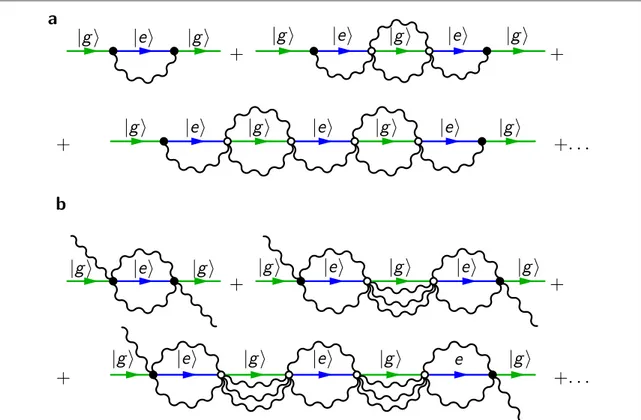
Figure 2. Feynman diagrams contributing to the energy correction of the ground state(a), and of the first excited state (b) of the Rabi Hamiltonian. Each bubble diagram, corresponding to a matrix element ofGˆ0, describes the intermediate virtual excitations enriching

the ground and thefirst excited states. The virtual excitations originate from the counter-rotating terms in the interaction Hamiltonian.

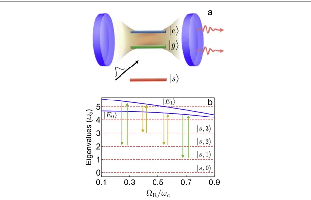
assumed to be much larger than the cavity-mode resonance frequency such that the cavity does not interact significantly with the atom in the lowest energy state∣sñ(see figure3(a)). The interaction of this transition with

tha cavity can be further reduced considering three-level atoms with dipole moments m_sg,m_se m_ge. As we will show, the additional state∣sñenables an effective on/off-switch of the atom-cavity interaction. The system Hamiltonian is simplyHˆC=HˆR +ws ∣s sñá ∣. This Hamiltonian is block-diagonal and its eigenstates can be separated into a non-interacting sector∣s n, ñ, with energyws+ nwc, where n labels the cavity photon number,

and dressed atom-cavity states∣Eiñ, resulting from the diagonalization of the Rabi Hamiltonian(see figure3(b)). The direct excitation of the atom by applied electromagnetic pulses is described by the Hamiltonian



= +

ˆ _{( )( ˆ ˆ ) ( )}

Hd d t Vsg V ,se 8

whereVˆsg=msg(∣g sñá + ñá∣ ∣s g∣),Vˆse =mse(∣e sñá + ñá∣ ∣s e∣), and msgandmseare the dipole moments(here assumed to be real) for the transitions ñ « ñ∣s ∣g and ñ «∣s ∣e , respectively. We consider quasi-monochromaticñ

pulses d( )t =A t( )cos(wt), whereA t( )is a Gaussian envelope. We only consider pulses which are out of resonance with the transition ñ «∣g ∣e and neglect this transition in equationñ (8). If the system is prepared in a

dressed state∣Eiñ, the driving HamiltonianHˆdcan induce transitions towards the noninteracting states∣s m, ñ:



å

Thus_Hˆ_d, when applied to a dressed state, is able to convert the virtual photons enriching the physical excitations into real ones which can be detected. This is possible becauseHˆdinduces transitions from the atomic states∣gñ

and∣eñ(coupled to the cavity) to the noninteracting state∣sñ. Of course, the transitions only occur if the driving-field frequency ω is resonant with the frequency of the corresponding transition ñ ∣Ei ∣s m, ñ. Note also that, if the artificial atom displays parity symmetry, only one of the two dipole moments (msgandmse) will be nonzero. However, in artificial atoms (e.g., flux qubits), parity symmetry can be easily broken [61].

In the absence of counter-rotating terms, a JC eigenstate with n excitations can only undergo transitions towards states with n photons:∣E_nñ ∣s n, ñ(form ¹ 0_sg ), or -n 1 photons:∣E_nñ ∣s n, - ñ1 (for m ¹ 0_se ). 2.5. Stimulated emission and reabsorption of virtual particles

Wefirst consider the system prepared in the ground state∣E0ñof the quantum Rabi Hamiltonian. This state can

be easily reached from the ground state∣sñby directly exciting the artificial atom with a resonant π-pulse [7]. As

Figure 3.(a) Schematic of the system in which a three-level atom is placed in a cavity. The upper two levels ñ∣e and ñ∣g of the atom resonantly couple to a single cavity mode. The effective atom-cavity interaction can be controlled by external electromagnetic pulses (arrow with a Gaussian pulse) inducing transitions from the cavity-interacting levels ñ∣g and ñ∣e to the noninteracting level ñ∣s and vice versa. These pulses can induce the emission of photons(red arrows) enriching the ground or the excited states of the Rabi Hamiltonian.(b) Lowest energy-levels of the system as a function of the normalised coupling strengthWR wcand the transitions

long as the system remains in the state∣E0ñ(even if it is not the ground state of the total Hamiltonian w

+ ñá

ˆ _{∣ ∣}

HR s s s), no cavity photons can be observed, since the photons in∣E0ñare virtual. An input pulse of

central frequency w E0-ws -2wccan induce a transition∣E0ñ ∣s, 2ñ, corresponding to a stimulated

emission process(see figure3(b)). The corresponding matrix elementás, 2∣ ˆ ∣Vsg E0ñ =msgág, 2∣E0ñ,

determining the transition probability, is proportional to the probability amplitudec_g,20 = ág, 2∣E0ñthat in the

Rabi ground state there are two virtual photons. By exploiting perturbation theory(see appendixC), this matrix

element can be approximated asás, 2∣ ˆ ˆ ( ) ˆ ∣V Gsg 0 Vnr g, 0ñ. From the Dyson series, we obtain

       á ñ = á ñ + á ñ + á ñ + ¼ ∣ ˆ ˆ ( ) ˆ ∣ ∣ ˆ ˆ ( ) ˆ ∣ ∣ ˆ ˆ ( ) ˆ ˆ ( ) ˆ ∣ ∣ ˆ ˆ ( ) ˆ ˆ ( ) ˆ ˆ ( ) ˆ ∣ ( ) s V G V g s V G V g s V G V G V g s V G V G V G V g , 2 , 0 , 2 , 0 , 2 , 0 , 2 , 0 . 10 sg sg sg sg 0 nr 0 0 nr 0 0 r 0 0 nr 0 0 r 0 0 r 0 0 nr

Figure4(a) displays the diagrams describing the first nonzero terms in this series. The red crosses represent

the action of the perturbation ˆVsg. These Feynman diagrams provide a clear interpretation of the emission process. The loops infigure2contain virtual photons which contribute to the energy correction of the state∣E0ñ

and∣E1ñ. As shown infigure4, the time-dependent perturbation ˆVsgis able to cut these loops. These diagrams show that the virtual photons in the loops are not just a technical feature of perturbation theory but describe internal physical processes, which can be interrupted by a suitable perturbation able to convert each virtual photon into an observable physical photon. Specifically, diagrams in figure4(a) together with the rightward

time-arrow describe the transition∣E0ñ ∣s, 2ñ, where two cavity photons are emitted. The same diagrams, but

with a leftward time-arrow, describe the transition∣s, 2ñ ∣E0ñ, where two cavity photons are reabsorbed into

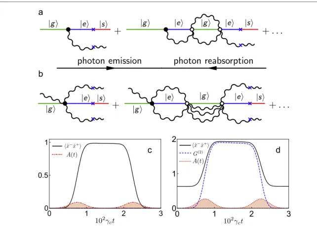
the Rabi ground state. The potential ˆVsginduces the breaking of two-photon loops, converting virtual photon Figure 4.(a) Diagrams contributing to the transition matrix element ás, 2∣ ˆ ∣Vsg E0ñ, associated with the transition∣E0ñ ∣s, 2ñ

(rightward time-arrow) where two cavity photons are emitted. The same diagrams but with a leftward time-arrow describe the reverse transition∣s, 2ñ ∣E0ñ, where two cavity photons get trapped into the Rabi ground state.(b) Diagrams contributing to the matrix

elementás, 3∣ ˆ ∣Vsg E1ñ, associated with the transitions∣E1ñ «∣s, 3ñ, where three photons enriching the lowest-energy excited state of

the Rabi Hamiltonian are emitted or reabsorbed back. The red crosses represent the perturbationVˆsg.(c) Numerical calculations of

the mean cavity-photon number(continuous black curve), and of the two-photon correlation function (dashed blue curve) corresponding to diagrams infigure4(a). The system is initially prepared in the state∣E0ñ. Aπ pulse, resonantly exciting the system from∣E0ñto∣s, 2 , is then sent. A secondñ (red) pulse induces the transition back from∣s, 2 toñ ∣E0ñ.(d) Numerical calculations of the

mean cavity-photon number(continuous black curve), and of the three-photon correlation function (dashed blue curve)

corresponding to diagrams infigure4(b). The system is initially prepared in the state ñ∣E1. Aπ pulse (filled curve), resonantly exciting

the system from∣E1ñto∣s, 3 , is then sent. A second pulse induces the transition back fromñ ∣s, 3 toñ ∣E1ñ. Here we usedWR wc= 0.15,

weg=wc, and geg=ggs=gc= ´2 10-5wc, wheregcis the decay rate for the cavity photons and geg,ggsare the decay rates for the

atom transitions ñ ∣e ∣g and ñ  ññ ∣g ∣s .

pairs into real ones. It is not able, however, to break one-photon loops. These can be broken by the potentialVˆse as shown below.

It is even more interesting to undress the excited states of the quantum Rabi model. This can provide access to the relationship between bare and physical excitations. Let us consider the lowest-energy excited state∣E1ñ

which, as we have shown in section2.2, is a single-particle state. Following the same steps as used in obtaining the series in equation(10), the diagrams in figure4(b) can be drawn. According to the Fermi golden rule, an input

pulse of central frequency w E1-ws-3wccan induce a transition∣E1ñ ∣s, 3ñ. The corresponding matrix

elementás, 3∣ ˆ ∣Vsg E1ñ =msg gc1,3is proportional to the probability amplitude that in the state∣E1ñthere are three

bare photons. By applying perturbation theory, it can be approximated as(see appendixC)

 

á ñ = - á - ñ

∣ ˆ ∣ ∣ ˆ ˆ ( ) ˆ ∣ ( )

s, 3 Vsg E1 1 s, 3 V Gsg 1 Vnr g, 1 . 11

The analytical perturbative calculations of the matrix elements ás, 2∣ ˆ ∣Vsg E0ñand ás, 3∣ ˆ ∣Vsg E1ñare described in

appendixC.

We complete the above analysis by presenting nonperturbative numerical calculations which accurately describe the dynamics of the undressing and re-dressing of the Rabi vacuum and of the Rabi lowest-energy excitation.

The spectrum and the eigenstates of the quantum Rabi HamiltonianHˆRhave been obtained by standard

numerical diagonalization in a truncatedfinite-dimensional Hilbert space. The truncation is realised by including only the N lowest-energy Fock states for the cavity mode. The truncation number N is chosen in order to ensure that the lowest M energy eigenvalues and corresponding eigenvectors, which are involved in the dynamical processes investigated here, are not affected significantly when increasing N. These results have been obtained using N=30, although numerical stability can also be achieved with a lower N.

We take into account the presence of dissipation channels, the presence of higher energy levels in the Rabi Hamiltonian, and the non-monochromaticity of the driving pulses. All the dynamical evolutions displayed in figures4(c) and (d) have been calculated numerically solving the master equation



rˆ˙ ( )t =i[ ˆ ( )r t ,Hˆ ]C + å_j ˆ ˆ ( )jr t [40,62,63], whereˆjare Liouvillian superoperators describing the different (atomic and photonic) dissipation channels. All calculations have been carried out with zero-temperature reservoirs, which is a reasonable assumption for systems at very low temperatures. For instance, for a system with a resonator at frequency wc (2p =) 10 GHzand temperature T=40 mK, the number of thermal photons is lower than 10−5. All the numerical calculations have been performed using

g =g =g = ´_{2 10}-w

eg gs c 5 c, where gcis the decay rate for the cavity photons and geg,ggsare the decay rates for the atomic transitions ñ ∣e ∣g and ñ  ññ ∣g ∣s . These small decay rates are still shorter than the typical decay

rates experimentally observed in state-of-the-art circuit QED systems(e.g., [64]). The density matrix, expressed

in the basis of the system eigenstates, is truncated in order to exclude all the higher-energy eigenstates which are not populated during the dynamical evolution. The system of differential equations resulting from the master equation is solved by using a standard Runge–Kutta method with step control.

We consider the system initially prepared in the state∣E0ñ(preparation starting from the ground state∣s, 0ñ

can be easily achieved by sending a suitableπ pulse). Then, a Gaussian pulse with central frequency

w =E0-ws-2wcinduces the transition∣E0ñ ∣s, 2ñ. Specifically, the pulse area required to obtain a

complete transition is p ∣ás, 2∣ ˆ ∣Vsg E0ñ∣. The pulse arrival-time corresponds to the time when the loops in the Feynman diagrams are cut. Figure4(c) displays the dynamics of the intracavity mean excitation numberáx xˆ ˆ- +ñ, which is directly related to the output photonfluxFout( )t =gcáx t x tˆ ( ) ˆ ( )- + ñ(where gcis the photon escape rate

through the cavity boundary), as well as the equal-time second-order correlation function

= á - + ñ

( ) ( ˆ ( )) ( ˆ ( ))

( )

G2 t x t 2 x t 2 _{[15]. Before the arrival of the Gaussian pulse (shaded red curve), the output photon}

flux is zero, since á_{E ∣ ˆ ˆ ∣x x}- + _Eñ = ₀

0 0 . After the arrival of the pulse, the photonflux becomes nonzero and

á - +ñ 

( ) ˆ ˆ

( )

G2 t x x _{, confirming that a two-photon state is actually generated as expected from the diagrams in}

figure4(a). When a second pulse is sent, the two photons are reabsorbed almost completely into the Rabi ground

state:∣s, 2ñ ∣E0ñ(diagrams in figure4(a) with the leftward time-arrow). Figure4(c) shows that a residual small

excitation remains in the system after the arrival of the second pulse. This can be attributed to the influence of cavity losses which give rise to a spontaneous transition∣s, 2ñ ∣s, 1ñ. As a result, a small butfinite population in∣s, 1 leads to áñ x xˆ ˆ- +ñ ¹0with_G( )2 =_{0. As expected, this residual excitation disappears in absence of}

dissipation.

Figure4(d) displays the dynamics starting from the system prepared in the state∣E1ñ. If the dipole moment m ¹ 0_es , this state can be reached directly from the ground state∣s, 0 by exciting the artiñ ficial atom with a

resonantπ-pulse. If m = 0_es , it is possible to reach the state in two steps(∣s, 0ñ ∣E0ñ ∣E1ñ). We observe that,

after the arrival of the Gaussian pulse(with central frequency w =E1-ws -3wc, and area p ∣ás, 3∣ ˆ ∣Vsg E1ñ∣),

the initially zero third-order correlation function_G( )3 _{approaches 6, the value corresponding to a three-photon}

are reabsorbed by sending an additional identical Gaussian pulse. We observe that, within the standard RWA,

 

á + - + +ñ =

∣ ˆ ( ) ˆ ( )∣x t x t 0.5

1 1 . Figure4(d) at t=0 displays a higher value. This is a peculiar effect of the USC

regime, where the intracavity mean excitation number is quadrature-dependent. In particular, it increases for ˆx measurements and decreases for measurements of the conjugate quadrature_yˆ=_i( ˆ_a†-_aˆ)_.

Having studied the above processes induced by ˆVsg, we now turn to those involvingVˆseinstead. Specifically, we consider the case where the dipole transition momentm_seis different from zero. Figure5shows these processes, with the action ofVˆserepresented in the diagrams by blue crosses. These processes are able to break one-photon loops, as illustrated infigure5(a), which shows the diagrams associated with the transition

ñ  ñ

∣E0 ∣s, 1, where a cavity photon is emitted(rightward time-arrow) and reabsorbed (leftward time-arrow).

Figure5(b) shows the diagrams associated with the transitions ñ «∣E1 ∣s, 2ñ, where two photons enriching the

lowest-energy excited state∣E1ñof the Rabi Hamiltonian are emitted or reabsorbed. The analytical perturbative

calculations of the matrix elements ás, 1∣ ˆ ∣Vse E0ñand ás, 2∣ ˆ ∣Vse E1ñare described in appendixD. In complete

analogy with what was shown infigures4(c) and (d), we present in figures5(c) and (d) nonperturbative

numerical calculations describing the dynamics of the undressing and re-dressing of the quantum Rabi vacuum and of the quantum Rabi lowest-energy excitation, taking into account the presence of dissipation channels, the presence of higher-energy levels, and the non-monochromaticity of the driving pulses. Wefirst consider the system starting in the state∣E0ñ, corresponding to an intracavity mean excitation number áx xˆ ˆ- +ñ =0. Then, a

Gaussian pulse with central frequency w=E0-ws -wcinduces a transition∣E0ñ ∣s, 1ñ. Specifically, the

pulse area required to obtain a complete transition is p ∣ás, 1∣ ˆ ∣Vse E0ñ∣. The pulse arrival-time corresponds to the time when the loops in the Feynman diagrams are cut. Figure5(c) displays the time evolution ofáx xˆ ˆ- +ñ.

Figure 5.(a) Diagrams contributing to the matrix element ás, 1∣ ˆ ∣Vse E0ñ, associated with the transition∣E0ñ ∣s, 1ñ(rightward

time-arrow) where a cavity photon is emitted. The same diagrams but with a leftward time-arrow describe the reverse transition

ñ  ñ

∣s, 1 ∣E0, where a cavity photon is absorbed into the Rabi ground state.(b) Diagrams contributing to the matrix element

ás, 2∣ ˆ ∣Vse E1ñ, associated with the transitions∣E1ñ «∣s, 2ñ, where two photons enriching the lowest-energy excited state∣E1ñof the

Rabi Hamiltonian are emitted or reabsorbed back. The blue crosses represent the perturbation ˆVse.(c) Numerical calculations of the

mean cavity-photon number(continuous black curve) corresponding to diagrams in figure5(a). The system is initially prepared in the

state∣E0ñ. Aπ pulse (shown in red), resonantly exciting the system from∣E0ñto∣s, 1 , is then sent. A second pulse induces theñ

transition back from∣s, 1 toñ ∣E0ñ.(d) Numerical calculations of the mean cavity-photon number (continuous black curve), and of the

three-photon correlation function(dashed blue curve) corresponding to diagrams in figure5(b). The system is initially prepared in the

state∣E1ñ. Aπ pulse (red filled curve), resonantly exciting the system from ñ∣E1to∣s, 2 , is then sent. A second pulse induces theñ

transition back from∣s, 2 toñ ∣E1ñ. For the other parameters of the simulation not specified here, the same values as in figure4were

used.

After the arrival of thefirst pulse,áx xˆ ˆ- +ñjumps and almost reaches the value 1. The equal-time second-order correlation function_G( )2( )_{t , not displayed, remains zero, confirming that a single-photon state is generated.}

Figure5(d) displays the dynamics starting from the system prepared in the state∣E1ñ. We observe that, after

the arrival of the Gaussian pulse(with central frequency w=E1-ws-2wcand area p ∣ás, 2∣ ˆ ∣Vse E1ñ∣), the

initially zero second-order correlation function_G( )2 _{approaches 2, the value corresponding to a two-photon}

state. This result confirms the occurrence of the transition ñ ∣E1 ∣s, 2ñ. Also in this case, the emitted photons are reabsorbed after an additional identical Gaussian pulse is sent.

We observe that both infigures4and5, a normalised coupling strengthWR wc= 0.15is sufficient to break

one-, two-, and three-photon loops, converting virtual photons into real ones with probability close to one. This value of the normalised coupling strength isWR wcroughly equal to the experimentally demonstrated values in

circuit-QED systems[24]. We note thatce,10 andce,21 are significantly larger thancg,20 andcg,31 , respectively. Hence the process induced byVˆsecan be observed even for smaller coupling strenghts.

3. Discussion

The results presented here show that the USC regime of cavity QED can be used to observe, in a direct way, how interactions dress the observable particles by a cloud of virtual particles. Such particle dressing is a general feature of QFT and many-body quantum systems. We have shown that, by applying external electromagnetic pulses of suitable amplitude and frequency, each virtual photon enriching a physical excitation can be converted into a physical observable photon. In this way, the hidden relationship between the bare and physical excitations can be unravelled and becomes experimentally testable. Virtual particles are represented by internal loops in Feynman diagrams. These loop or bubble diagrams describe internal processes where virtual photons are created and reabsorbed. The diagrams representing the conversion of virtual photons, dressing a physical excitation, into real ones can be obtained by cutting the loop diagrams describing energy corrections and taking thefirst half. Moreover, the stimulated reabsorption of real photons into the physical excitation, converting them to virtual photons, corresponds to the second half of the loop diagrams.

We limited our analysis to the dressed vacuum and to a one-particle state. It can be easily extended to study higher-energy excitations. Moreover, we considered only processes up to second-order perturbation theory in the counter-rotating potential ˆVnr. The present analysis can be generalised to describe higher-order processes,

involving more than three photons, which can take place if the light–matter interaction is sufficiently strong[35].

The most promising candidates for an experimental realisation of the proposed stimulated conversion effects are superconducting quantum circuits[65] and intersubband quantum-well polaritons. In particular,

phase-biasedflux qubits can reach the USC regime in circuit QED [66], as has been shown in experiments

[23,24,35,67]. Very recently, hybrid quantum circuits [68] withWR wegranging from 0.72 to 1.34 have been realised[35] by making use of the macroscopic magnetic dipole moment of a flux qubit, large

zero-point-fluctuation current of an LC oscillator, and large Josephson inductance of a coupler junction. In flux qubits, an externally applied magneticflux can be changed such that these artificial atoms acquire both the quantised level structure and the transition matrix elements required for the observation of the stimulated emission and reabsorption of virtual particles[7]. Specifically, the supplementary material of [7] contains a section where

numerical calculations show how an artificial atom (a flux qubit) with a specific flux offset can provide the required level spacing and dipole moments to observe the effect. We have checked that working far from the sweet spot(around zero flux-offset) does not affect the results significantly. In addition, we observe that it is not necessary that level∣sñhas lower energy than∣gñ. In this case, the standard configuration of flux qubits near the sweet spot can provide the required level structure and dipole moments[23,24,35]. The description of the

stimulated emission and reabsorption of virtual photons presented here also holds if∣sñhas higher energy than the∣gñand∣eñstates.

The USC regime can also be reached for intersubband transitions in undoped quantum wells[69]. In this

system, an optical resonator in the terahertz spectral range is resonantly coupled to transitions between the two-lowest energy conduction subbands of a large number of identical undoped quantum wells. In this case, the upper valence subband plays the role of the lowest energy state∣sñ(see figure3). Ultrafast optical pulses can

induce transitions between the valence and conduction subbands prompting the conversion from virtual to real photons and vice versa.

Such experiments would provide deep insight into fundamental aspects of interaction processes in QFT and quantum many-body systems. They would pave the route for quantum emulation[70,71] of fundamental

Acknowledgments

FN was partially supported by the RIKEN iTHES Project, MURI Center for Dynamic Magneto-Optics via the AFOSR Award No. FA9550-14-1-0040, the Japan Society for the Promotion of Science(KAKENHI), the IMPACT program of JST, CREST grant No. JPMJCR1676, and the John Templeton Foundation. AFK acknowledges support from a JSPS Postdoctoral Fellowship for Overseas Researchers.

Appendix

In these appendix sections, wefirst restate some properties of the quantum Rabi model and its diagrammatic representation, expanding on the discussion in the main text. We then proceed to explicitly calculate analytically the second-order correction to the lowest energy eigenvalues and comparing them to full numerical

calculations. We also calculate matrix elements associated with the external drive used to stimulate the emission and reabsorption of the virtual particles dressing the excitations in the system.

Appendix A. Hamiltonian and basic diagrams

The interaction Hamiltonian of the quantum Rabi model is

s

= W +

ˆ _{( ˆ}† _{ˆ) ˆ ( )}

V R a a x, A1

where WRis the coupling strength and sˆx=sˆ++sˆ-= ñá + ñá∣e g∣ ∣g e∣. Referring to the case

wc »weg ºwe-wg, the interaction Hamiltonian can be separated into a resonant and a nonresonant contribution:Vˆ =Vˆr+Vˆnr, whereVˆr= WR( ˆ ˆa†s-+aˆ ˆ )s+ , andVˆnr= WR( ˆ ˆa†s++aˆ ˆ )s-. This interaction term

has a structure which is very similar to that of the QED interaction potential, although it is simpler. The quantum Rabi model can be viewed as a prototypical QED system where there is only one photon mode and a two-state electron. Therefore, we expect that the Feynman diagrams for the Rabi Hamiltonian will be a simplified version of the QED diagrams.

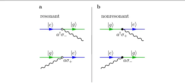
As in QED, there is only one vertex type with three lines: one wavy(photonic) line, one solid line with an incoming arrow, and one solid line with an outgoing arrow. The vertices(of the same type) corresponding to the four terms in the interaction Hamiltonian are displayed infigureA1. The upper diagram infigureA1(a)

describes the spontaneous emission process and the lower one the absorption process. Starting from these four building blocks, it is possible to describe higher-order processes as in QED. However, in cavity QED there are processes that are not described in a complete way by Feynman diagrams directly derived from this form of the interaction Hamiltonian. Specifically, the presence of a resonator supporting discrete modes opens up the possibility of observing processes involving more than one photon in the same mode. Stimulated emission, the process underlying laser action, is one of these. It is a one-photon process∣e n, ñ ∣g n, + ñ1, where, however, the n photons in the initial state stimulate the downward transition of the atom, affecting the transition rate

Figure A1. Diagrams corresponding to the four terms in the interaction Hamiltonian of the quantum Rabi model. The horizontal lines represent the qubit states and the wavy lines the cavity photons.(a) Diagrams corresponding to those terms in the interaction Hamiltonian that conserve energy whenwc=weg.(b) Diagrams for the termsµaˆ ˆ†s+andaˆ ˆs-, which conserve neither energy nor the number of excitations. Their elimination corresponds to the RWA.

which becomes proportional ton+1. The Feynman diagram describing the process is the same one describing spontaneous emission(n = 0), shown in figureA1(a). However, the transition rate for stimulated emission is

+

n 1times larger than that of spontaneous emission. Hence the Feynman diagram in the absence of additional rules is not able to uniquely determine the transition amplitude for this process.

A possible solution is to expand the photon creation and destruction operators in equation(A1) in the Fock

basis. The resulting interaction operator is

å

where aˆ+( )n =aˆ ∣† n nñá ∣= n+1 ∣n+ ñá1 n∣, and aˆ-( )n =a n nˆ ∣ ñá ∣= n n∣ - ñá1 n∣(notice that aˆ_-( )0 =0). This form of the interaction Hamiltonian consists of a sum of products of (upward or downward) atomic and photonic transition operators; thus photonic and atomic transitions are treated on an equal footing. In this case, each vertex is associated to two transition operators. For example, the vertex describing the

transition∣e, 1ñ ∣g, 2 is shown inñ figureA2(a): the wavy lines describe the incoming and the outgoing

photon states, while the continuous line with the arrows describes the incoming and outgoing electronic states. The vertex infigureA2(a) describes a stimulated emission process. Since the photon wavy lines are labelled by

the photon number, an alternative(perhaps more visual) way to draw diagrams is to drop the photon label and draw a wavy line for each incoming or outgoing photon line as shown infigureA2(b). In this case, the vertices

will havenin=nincoming andnout =n1outgoing wavy lines. Each vertex(full/empty circle) contributes

with a factor n V∣ ˆr nr∣, wheren=max(nin,nout).

The Green’s function for the system in the absence of interaction,

w w º á ñ = - + ˆ _{( ) ∣ ˆ ∣} ( ) ( ) ( ) G z q n G q n z n , , 1 , A3 q n qg 0 c

where wqg=wq-wg, withq=e g, , corresponds to a loop diagram with n wavy lines and one straight arrow. InfigureA3, we show the two loop diagrams corresponding toGe( )2 andGg( )1.

Appendix B. Second-order correction to the energy eigenvalues

The well-known second-order correction to the nth energy eigenvalue is

å

Figure A2. Diagrams corresponding to the the transition∣e, 1ñ ∣g, 2 .ñ(a) Diagram with one incoming and one outcoming wavy line, each labelled respectively with the number of photons involved in the process.(b) Diagram for the same process, but in this case each wavy line represents one single photon.

Figure A3. Examples of diagrams corresponding to the Green’s function. (a) Diagram foráe, 2∣ ˆ ∣G0 e, 2ñ.(b) Diagram for

where the prime in the summation means that the values k=n have to be excluded. For the first-order correction to the eigenfunction we have

å

Following[58], defining the projection operator onto the space orthogonal to∣nñ,Qˆn=1ˆ -∣n nñá ∣, equation(B2) becomes ñ = ñ ∣E_n( )1 Q G E Q V E ,ˆ ˆ ( ) ˆ ˆ ∣n n0 n n (B3) where = -ˆ ( ) ˆ ( ) G E E H 1 B4 n n 0 0 ₀ 0

is the unperturbed Green’s function calculated for E0n, the unperturbed eigenenergy of the system.

Using the definition of the Green’s function from equation (B4) and the projection operators, equation (B1)

becomes

DE_n( )2 = áEk∣ ˆ ˆ ˆ (VQ G E Q V E .n n) ˆ ˆ ∣n nñ (B5) We apply these results to the JC Hamiltonian perturbed by the non-resonant potential ˆVnr. In this case, the

unperturbed HamiltonianHˆ0becomesHˆJC=Hˆ0+Vˆr, whose eigenvalues and eigenstates are n and  ñ∣ n , respectively. We have

+ñ = ñ + - ñ -ñ = - ñ +  - ñ

∣ _n n∣g n, n∣e n, 1 ∣ n n∣g n, n∣e n, 1 . (B6)

The action of the non-resonant potential on these eigenstates is

+ñ = W  + ñ + - ñ ˆ ∣ ( ∣ ∣ ) ( ) Vnr n R ne n, 1 ng n, 2 B7 and -ñ = W - + ñ + - ñ ˆ ∣ ( ∣ ∣ ) ( ) Vnr _n R ne n, 1 ng n, 2 . B8

From the last two equations, we deduce that the non-resonant potential ˆVnrdetermines transitions from the

subspace n(spanned by _n) to (n+2) or (n−2) subspaces. As a consequence, we have ñ = ñ

ˆ ˆ ∣ ˆ ∣ ( )

Q Vn nr n Vnr n . B9

Owing to this property, equation(B5) becomes

    D = D  = á   ñ ∣ ˆ ˆ ( ) ˆ ∣ ( ) ( ) ( ) _{V G V , B10} n n n n 2 2 nr nr where  = - - = - - -ˆ ( ) ( ˆ ) ( ˆ ˆ ) ( ) G n n HJC 1 n H0 Vr 1 B11

is the JC Green’s function. Equation (B10) can be easily calculated exploiting the matrix elements of the JC

Green’s function by using the JC eigenstates. We do not follow this procedure because our scope is to show, through a diagrammatic analysis, the structure of the virtual processes that contribute to such a correction. For this purpose, we exploit the Dyson equation for the JC Green’s function, considering now the resonant potential

ˆ

Vras the perturbation, and the Green’s function in the absence of interactionGˆ ( )0 n =(n-H0)-1:

= + +

ˆ ˆ ˆ ˆ ˆ

G G0 G V G0 r 0 .... Equation(B10) can thus be expanded as

       D = á   ñ + á    ñ + ∣ ˆ ˆ ( ) ˆ ∣ ∣ ˆ ˆ ( ) ˆ ˆ ( ) ˆ ∣ ( ) ( ) V G V V G V G V .... B12 n 2 n nr 0 n nr n n nr 0 n r 0 n nr n

Using equation(B12), the lowest-order (second-order) correction to the ground state∣g, 0ñenergy due to the non-resonant potential ˆVnrcan be expressed as

D = á( )₀2 g, 0∣ ˆV G E Vnr ˆ ( ) ˆ ∣0 nr g, 0ñ = ág, 0∣ ˆV G Vnr ˆ ˆ ∣0 nr g, 0ñ + ág, 0∣ ˆV G V G Vnr ˆ ˆ ˆ ˆ ∣0 r 0 nr g, 0ñ +.... (B13) By using the identity operator and exploiting the explicit expression of ˆVnr, equation(B13) can be expressed as

D = á( )₀2 g, 0∣ ˆ ∣Vnr e, 1ñáe, 1∣ ˆ ∣G e, 1ñáe, 1∣ ˆ ∣Vnr g, 0ñ = W áR2 e, 1∣ ˆ ∣G e, 1 .ñ (B14) In order to calculate D( )02, we observe that

ág, 0∣ ˆ ∣Vnr e, 1ñ = áe, 1∣ ˆ ∣Vnr g, 0ñ = WR. (B15) The remaining term, áe, 1∣ ˆ ∣G e, 1 , is a convergent geometric series that is calculated in appendixñ E. We obtain

w w D = W W - ( ) ( ) 2 1 2 1. B16 02 R 2 c R2 c2

ForWR wc < 1, D( )02 can be approximated to second order in WR: w D » -( ) W ( ) 2 . B17 02 R 2 c

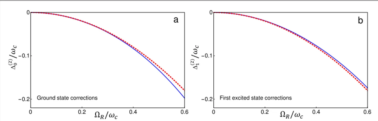
InfigureB1, we show the comparison between the exact(numerical) and approximated (diagrammatic) calculation of the correction term to the ground state energy.

This approach can also be applied to the excited states. We consider thefirst excited state. Using equation(B10), we are able to calculate the correction up to second order in the potential ˆVsgto E1; we have

    

D = á - - -ñ = á - ñ

∣ ˆ ˆ ( ) ˆ ∣ ∣ ˆ ˆ ( ) ˆ ∣ ( )

( ) _{V G V g, 1 V G V g, 1 . B18}

12 1 nr 1 nr 1 12 nr 1 nr

Observing thatV e, 0ˆ ∣nr ñ = 0,V gˆ ∣nr , 1ñ = 2WR∣e, 2ñ, and ∣ 1-ñ = -1∣g, 1ñ +1∣e, 0ñ, we have

-ñ = - W ñ ˆ ∣ ∣ ( ) Vnr 1 2 1 Re, 2 . B19 Equation(B18) becomes        D = á ñ = á ñ = W á ñ - - - -∣ ˆ ˆ ( ) ˆ ∣ ∣ ˆ ˆ ( ) ˆ ∣ ∣ ˆ ( )∣ ( ) ( ) V G V g V G V g e G e , 1 , 1 2 , 0 , 0 . B20 12 1 nr 1 nr 1 12 nr 1 nr 12 R2 1

The energy correction D( )

12 can be easily evaluated by directly using ˆ ( )G z or by summing up the infinite

contributions arising from the Dyson series, described by the diagrams(see appendixE, equation(E11)).

In the absence of detuning, we have for thefirst excited state

 ñ =- - ñ + ñ ∣ 1 ( ∣g ∣e ) ( ) 2 , 1 , 0 , B21 1 with energy -=w - W _{. (B22)} 1 c R We obtain w w w D = -W W + - W - W ( ) ( ) 2 4 4 2 . B23 12 R2 R c c 2 R c R2

ForWR wc< 1, D( )12 can be approximated to second order in WR: w D » -( ) W ( ) 2 . B24 12 R 2 c

A comparison between the approximate analytical energy corrections and the corresponding nonperturbative numerical calculations can be found infigureB1.

Appendix C. Additional perturbation

V

^

allowing transitions from

∣g

ñ

to

∣s

ñ

Using equation(B1), the correction to the JC eigenstate  ñ∣ n up to thefirst order in the non-resonant potential becomes,

Figure B1. Comparison between the exact_{(numerical) and approximated (diagrammatic) calculation of the correction terms for (a)} the ground-state energy and(b) the first excited state. The blue continuous lines describe the numerical calculation, while the red dotted lines describe the approximate one.

 

ñ = ñ

∣En( )1 Q Gˆ ˆ ( ) ˆ ∣n n Vnr n . (C1)

We now consider the direct excitation of the artificial atom by applied electromagnetic pulses, described by the Hamiltonian



= +

ˆ _{( )( ˆ ˆ ) ( )}

Hd t Vsg V ,se C2

whereVˆsg=msg(∣g sñá + ñá∣ ∣s g∣),Vˆse =mse(∣e sñá + ñá∣ ∣s e∣), and msgandmseare the dipole moments(here assumed to be real) for the transitions ñ « ñ∣s ∣g and ñ «∣s ∣e , respectively.ñ

First, we consider the case with the system prepared in the state  ñ =∣ 0 ∣g, 0ñ. The time-dependent

perturbation can induce additional transitions whose rate can be evaluated with the Fermi golden rule. In the absence of the counter-rotating interaction terms ˆVnr,Hˆdcan induce only zero-cavity-photon

transitions∣g, 0ñ «∣s, 0ñ. When including the counter-rotating terms, additional transitions are activated. For example, the transition∣E0ñ «∣s, 2ñacquires a nonzero matrix element ás, 2∣ ˆ ∣Vsg E0ñ, where∣E0ñis the lowest

energy state of the Rabi Hamiltonian. It can be calculated perturbatively in ˆVnr, approximating∣E0ñtofirst order

in ˆVnr(see equation (B3)):  ñ ñ + ñ ∣E0 ∣g, 0 Gˆ ( ) ˆ ∣0 V gnr , 0 . (C3) We obtain  m  ás, 2∣ ˆ ∣Vsg E0ñ = ás, 2∣ ˆ ˆ ( ) ˆ ∣V Gsg 0Vnr g, 0ñ = WR sgág, 2∣ ˆ ( )∣G 0 e, 1 .ñ (C4) The corresponding Dyson series is

     w w á ñ = á ñ + á ñ+ ¼ = W - - W = W - W ∣ ˆ ( )∣ ∣ ˆ ( )∣ ∣ ˆ ( ) ˆ ˆ ( )∣ ( ) ( ) g, 2 G e, 1 g, 2 G e, 1 g, 2 G V G e, 1 2 2 2 2 4 2 . C5 0 0 0 0 0 r 0 0 R 0 c 2 R2 R c 2 R 2

The comparison between the exact(numerical) and approximated (diagrammatic) calculation of this matrix element is shown infigureC1.

We now consider the case with the system prepared in the state  ñ =∣ -1 ( ∣-g, 1ñ +∣e, 0ñ)

1

2 , whose energy

is -₁ =wc- WR. The time-dependent perturbation can induce additional transitions whose rate can be

evaluated with the Fermi golden rule. In the presence of ˆVnr, additional transitions, such as∣E1ñ «∣s, 3ñ, become

activated. The matrix element for this transition is ás, 3∣ ˆ ∣Vsg E1ñ. It can be calculated perturbatively in ˆVnr,

approximating∣E1ñtofirst order in ˆVnr(see equation (B3)):

   ñ_ -ñ + - -ñ ∣E1 ∣ 1 Gˆ ( ) ˆ ∣1 Vnr 1 . (C6) Observing that  ñ = -- ñ - ñ = -W ñ ˆ ∣ ( ˆ ∣ ˆ ∣ ) ∣ ( ) V 1 V g V e e 2 , 1 , 0 , 2 , C7 nr 1 nr nr R

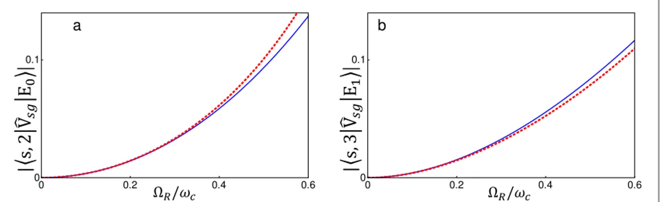
Figure C1.(a) Comparison between the exact (numerical, blue continuous curve) and approximated (diagrammatic, red dotted curve) calculation of the transition element á∣s, 2∣ ˆ ∣V Esg 0ñbetween the state∣s, 2ñ(where ñ∣s is now the real ground state) and∣E0ñ(the

cavity-dressed ground state_{) due to the additional}Vˆsgpotential as a function of the coupling parameter normalised to the cavity

resonance frequency.(b) Comparison between the exact (numerical) and approximated (diagrammatic) calculation of the transition element∣ás, 3∣ ˆ ∣V Esg 1ñ∣between the state∣s, 3ñ(where ñ∣s is now the real ground state) and ñ∣E1(the cavity-dressed first excited state)

due to the additionalVˆsgpotential as a function of the coupling parameter, normalised to the cavity resonance frequency. This

comparison confirms the validity of the approximate diagrammatic approach. For the sake of simplicity, here we usedWRm_sg= 1.

where we have used the relationsV gˆ ∣nr , 1ñ = 2WR∣e, 2ñandV e, 0ˆ ∣nr ñ = 0, we obtain

  m 

á ñ = á - -ñ = -W á - ñ

∣ ˆ ∣ ∣ ˆ ˆ ( ) ˆ ∣ ∣ ˆ ( )∣ ( )

s, 3 Vsg E1 s, 3 V Gsg 1 Vnr 1 R sg g, 3 G 1 e, 2 . C8

The corresponding Dyson series is(see appendixEand equation(E12))

     w w á ñ = á ñ + á ñ+¼ = W - - W = W W + - W - - - -∣ ˆ ( )∣ ∣ ˆ ( )∣ ∣ ˆ ( ) ˆ ˆ ( )∣ ( ) ( ) ( ) g, 3 G e, 2 g, 3 G e, 2 g, 3 G V G e, 2 3 3 3 3 2 3 . C9 1 0 1 0 1 r 0 1 R 1 c 2 R2 R R c 2 R2

Appendix D. Additional perturbation

V

^

allowing transitions from

∣e

ñ

to

∣s

ñ

We now consider a situation similar to the one analysed previously. In this case, a transition ñ «∣s ∣e is detunedñ

at a much higher energy than the cavity resonance. The part of the time-dependent potential inducing the ñ « ñ

∣s ∣e transitions isV tˆ ( )¢ =( ) ˆt Vse. In the absence of the counter-rotating interaction terms ˆVnr,V tˆ ( )¢ can

induce zero-cavity-photon transitions∣e, 0ñ «∣s, 0ñ.

In the presence of ˆVnr, additional transitions, such as∣E0ñ «∣s, 1ñ, can be activated. The matrix element for

this transition is ás, 1∣ ˆ ∣Vse E0ñ. It can be calculated perturbatively in ˆVnr, approximating∣E0ñto thefirst order in

ˆ Vnr(see equation (B3)):  ñ ñ + ñ ∣E0 ∣g, 0 Gˆ ( ) ˆ ∣0 V gnr , 0 . (D1) We have  m  ás, 1∣ ˆ ∣Vse E0ñ = ás, 1∣ ˆ ˆ ( ) ˆ ∣V Gse 0 0 Vnr g, 0ñ = WR seáe, 1∣ ˆ ( )∣G0 0 e, 1 .ñ (D2) Exploiting the Dyson series for the Green’s function, we obtain

   

áe, 1∣ ˆ ( )∣G 0 e, 1ñ = áe, 1∣ ˆ ( )∣G0 0 e, 1ñ + áe, 1∣ ˆ ( ) ˆ ˆ ( )∣G0 0V Gr 0 0 e, 1ñ +.... (D3) In this series, owing to the nature of the resonant potential, only the odd terms are non-zero. We have:

 

å

The diagrammatic analysis of this process is shown infigure5of the main part of the paper. Using the results of appendixE, the Dyson series calculation of equation(D2), at resonance (wcweg), gives

 m m w w á ñ = W á ñ = W W -∣ ˆ -∣ ∣ ˆ ( )∣ ( ) s, 1 V E e, 1 G e, 1 2 . D5 se 0 R se 0 se R c R 2 c 2

Appendix E. Calculation of the

G

^

matrix elements using the Dyson equation

In this section, we perform all the calculations for the determination of the correction to the self-energy to second order in ˆVnr. We have to sum all the elements of the infinite series. The generic matrix element is

áe, 1∣ ˆ ( )[ ˆ ˆ ( )] ∣G z V G z n e, 1 .ñ (E1)

0 r 0

We observe that the matrix element will be zero if ˆVrappears an odd number of times, i.e.,

á_{e, 1∣ ˆ ( )[ ˆ ˆ ( )]G z V G z} n+ _{∣ e, 1}ñ =_{0 forn}>_{0. (E2)}

0 r 0 2 1

Hence we may perform the calculation for the self-energy considering only the even-power terms. In addition, we observe that