http://www.scirp.org/journal/me ISSN Online: 2152-7261
ISSN Print: 2152-7245
The “Surprise Effect” of Macro Indicators on the
Options Implied Volatilities Dynamics: A Test
on the United States-Germany Relationship
Michele Patanè
1, Mattia Tedesco
1, Stefano Zedda
21Department of Business and Law, School of Economics and Management, University of Siena, Siena, Italy 2Department of Business and Economics, University of Cagliari, Cagliari, Italy
Abstract
This paper analyzes the “surprise effect” of some macroeconomic indicators on the US and Germany stock indexes options implied volatility, by means of a VAR model and IRFs between the two volatility indexes. Results show a sig-nificant influence of some specific macroeconomic “surprise effects” so that the US volatility has a positive influence on the German one, but not vice ver-sa. With reference to the first considered period, January 2008-May 2012, characterized by higher volatility, the German market analysis shows a direct link between the “surprise effect” of the IFO Business Climate Index and the VDAX-NEW index changes. As regard the second time period (June 2012- December 2014), characterized by lower volatility, the significant macro “sur-prise effects” are related to the industrial sector (US Retail Sales, German Pro- ducer Price) and the job market (US Non-Farm Payroll). These results on the linkages between the macro “surprise effects” and the volatility indexes can be useful for implementing more effective short-term speculative and hedging strategies, based on the “surprise effect” direction and his link with the volatil-ity index.
Keywords
Implied Volatility, Macro Surprise Effect, Markets Influences, VIX Index, VDAX-NEW Index
1. Introduction
Several researches have studied the possible relation between some macroeco-nomic variables and the pricing dynamic of some instruments listed on financial markets. Mapping these linkages can be of great importance for a better predic-tion and anticipapredic-tion of the future market evolupredic-tion, and in supporting opera-How to cite this paper: Patanè, M.,
Te-desco, M. and Zedda, S. (2017) The “Sur-prise Effect” of Macro Indicators on the Options Implied Volatilities Dynamics: A Test on the United States-Germany Rela-tionship. Modern Economy, 8, 590-603. https://doi.org/10.4236/me.2017.84044 Received: March 16, 2017
Accepted: April 24, 2017 Published: April 27, 2017 Copyright © 2017 by authors and Scientific Research Publishing Inc. This work is licensed under the Creative Commons Attribution International License (CC BY 4.0).
http://creativecommons.org/licenses/by/4.0/
tors in their selection of the most effective investment strategies, and/or in the planning of hedging transactions.
Unlike traditional studies, which focus on the influence between the domestic “macro surprise effects” and the volatility dynamic of their own markets, the first focus of this paper is on the possible links between the US volatility index and the German one. In fact, some previous studies (see e.g. [1][2][3][4] and
[5]) evidenced that the US economy have a significant influence on the world-wide economic trends, which keeps the operators’ attention on the major US macro news.
So we firstly analyzed the linkages between the two volatility indexes, by means of a vector autoregressive model (VAR), for testing for any connections between the volatility indexes, and for evaluating the possible links between these indexes and the foreign surprise effects. In this way, the German volatility dynamic was examined with reference to both the domestic “surprise effects” and the influence of the US volatility index, showing that the VIX index actually influences the VDAX-NEW index.
A second analysis is performed by means of two specifically designed equa-tions, based on the previous results, and tested on two time periods characte-rized by high and low volatility,
The reminder of the paper is organized as it follows: Section 2 is devoted to the related literature, Section 3 describes the dataset, Section 4 presents the pre-liminary analysis and the econometric approach, Section 5 reports the empirical results and Section 6 concludes.
2. Literature Review
A large part of the literature has focused on the influence that “planned” news have on the dynamics of the stock markets. These studies can be split in two main research streams. The studies belonging to the first research stream are based on historical volatilities, or functions of past returns, as financial market uncertainty measures. Among these, the most significant are:
• [6], which examines the relation between the stock returns volatility and the level of economic activity. The analysis is carried out for the time period 1857-1987, using monthly estimates of returns standard deviation of the Standard & Poor's and the Dow Jones. The author shows how the stock mar-ket volatility is linked to the general state of the economy and how it tends to rise during recessions;
• [7] examines the effects of monetary policy announcements on the stock market volatility. The study is carried out for the time period June 1989 - December 1998. The author examines the FOMC (Federal Open Market Committee) announcements, related to deposits interest rates, and the daily returns volatility of the S&P500, estimated through a GARCH model. Its re-sults show that the macro surprise effects tend to grow the stock market vola-tility. Specifically, an higher than expected interest rate increase (positive surprise), has a greater effect on the volatility than a lower decrease (negative
surprise);
• [4] focus on the stock markets integration. The authors studied the equity indexes of 35 countries, divided into six different groups, from July 1995 to March 2002, through a GARCH model. They obtained volatility dynamic es-timate is then analyzed with reference to some US macroeconomic indica-tors. Results show how the financial markets integration is due to the US macro bulletins, and how both the US and the foreign investors are interested in the US economic situation because of its leading role on the worldwide economy;
• [8] examine the impact of domestic and foreign macroeconomic news an-nouncements on the Istanbul Stock Exchange in the period 2002-2010. They found that foreign announcements don’t have a significant effect, whereas domestic announcements induce higher volatility in the market.
The second research stream uses the options implied volatility indexes as a fi-nancial market uncertainty measure. The implied volatility is in fact a measure of the stock market uncertainty due to the market’s expectation on the average volatility of returns until the option expiration date (see [9]). These indexes can help in overcoming some problems in the returns volatility estimation methodologies. They also give us the chance to invest on them, through vari-ous types of financial derivatives instruments. Among these studies the most relevant are:
• [10], who show that in the period June 1991-December 1992 the volatility of options listed on the European Options Exchange (EOE) has a significant in-crease in the days preceding the announcements, which reaches the maxi-mum on the day before the announcement, and decreases gradually to the long-term average in the days following the announcement;
• [3] examined the S&P 100’s volatility behavior through the VIX index, in the days around the announcements of the FOMC, within the period from Janu-ary 1996 to December 2000. Their results confirm the hypothesis that the implied volatility tends to increase during the days before the FOMC meet-ings and decrease the following days;
• [11] analyzed the monthly VIX index dynamic in the period January 1986- December 2002, with reference to the unexpected component of some ma-croeconomic variables. Their results show that the unexpected increase of the non-farm employment involves a volatility index increase;
• [12] extend the study carried out by [3] until September 2006. The results of this study confirm the hypothesis of a significant decrease of the volatility during the day of the FOMC meetings;
• [13], who study the relationship between the US and Taiwan volatility index (VIX and TVIX), using a Correlated Bivariate Poisson Jump model, finding that the changes in the TVIX are deeply affected by the past information on the changes in the VIX.
The analysis developed in this paper can be classified in the second research stream. It analyzes the monthly dynamics of the implied volatility of options on
the S&P500 index (VIX) and the DAX30 (VDAX-NEW) index, and its linkages to the unexpected component1 of some macroeconomic variables. We
consi-dered the volatility indexes on a monthly basis due to the greater market liquidi-ty for derivative instruments listed on these indexes, to the higher number of negotiations made by operators, and to the frequency of macroeconomic data2
issued by the government statistical departments.
3. Data
The analysis is performed with reference to the US implied volatility (VIX) in-dex, the German implied volatility (VDAX-NEW) index and the macroeconom-ic announcements, from January 2008 to December 2014, as extracted from the Thompson Reuters-Eikon platform.
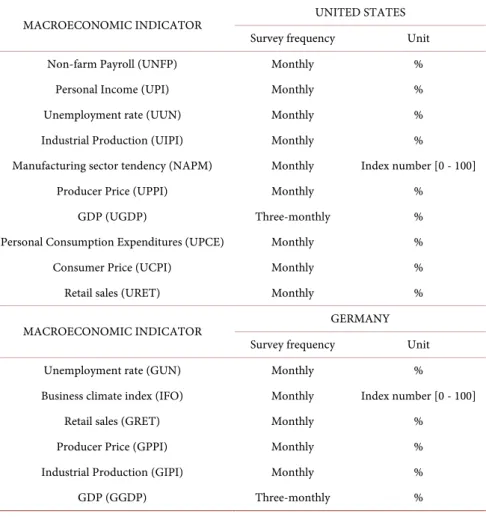
Table 1 lists the macroeconomic indicators considered in this analysis. These
Table 1. US and German macroeconomic indicators.
MACROECONOMIC INDICATOR UNITED STATES
Survey frequency Unit
Non-farm Payroll (UNFP) Monthly %
Personal Income (UPI) Monthly %
Unemployment rate (UUN) Monthly %
Industrial Production (UIPI) Monthly %
Manufacturing sector tendency (NAPM) Monthly Index number [0 - 100]
Producer Price (UPPI) Monthly %
GDP (UGDP) Three-monthly %
Personal Consumption Expenditures (UPCE) Monthly %
Consumer Price (UCPI) Monthly %
Retail sales (URET) Monthly %
MACROECONOMIC INDICATOR GERMANY
Survey frequency Unit
Unemployment rate (GUN) Monthly %
Business climate index (IFO) Monthly Index number [0 - 100]
Retail sales (GRET) Monthly %
Producer Price (GPPI) Monthly %
Industrial Production (GIPI) Monthly %
GDP (GGDP) Three-monthly %
1As suggested by [7] and [11].
2As the macro news are released on different days of the month, their impact can be captured using
monthly data of the volatility indexes. Assuming the news occur during the life of the option, fol-lowing Merton (1973) the average volatility until the option expiration date can be expressed as the average of the stock returns variances on the normal trading days and the news release days:
2 2 2
average normal news1 news n
1 1
t n
t t t
indicators, widely used in the past literature, refer to performances that have al-ready occurred, but able to synthesize the business cycle dynamics, as they in-clude information concerning the economic growth and inflation.
The “surprise effect” here considered refers to the news bringing new infor-mation, so to the cases when some index report a value which is different from the market consensus, derived from the previous information. It can thus be formally defined as the difference3 between the released announcement and the
market expectations for each macro indicator, as it follows: Surprise Effect=Realized Value−Expected value
As regards to volatility indexes, we consider the VIX index4 and the VDAX-
NEW index, which measure the market's expectations about the implied volatil-ity of the options with 30 days expiry listed, respectively, on the S&P500 and the DAX30.
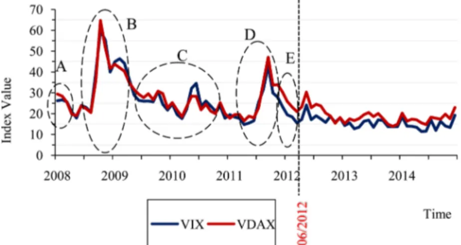
The volatility indexes dynamics for 2008-2014 are represented in Figure 1. The graphical analysis of the indexes show that the volatility trends have sig-nificantly changed during the considered time period, being characterized by a high volatility5 up to May 2012, and by a lower volatility since then to the end of
the considered time span (December 2014).
Specifically, there are five high volatile sub-periods: A corresponds to the Bear Stearns acquisition by means of JP Morgan Chase; B corresponds to the Lehman Brothers failure on 15 September 2008; C corresponds to the recession in Europe and in the United States; D and E correspond to the different monetary policies in both Europe and US.
Figure 1. Options implied volatility dynamic on S&P 500 (VIX) and DAX 30 (VDAX-
NEW).
3The surprise effect is considered as positive if the released value is higher than the market
expecta-tions, while a negative surprise effect refers to cases where the released value is lower than the mar-ket expectations.
4The VIX Index is listed by the CBOE (Chicago Board Options Exchange) and it was developed in
cooperation with Goldman Sachs. The index forecasts the expected volatility through a prices weighted average of out-of-the-money call and put options, which contain information about the volatility smirk.
5The first period high volatility is due to trigger factors related to the markets and the
As in [1] we thus performed our analysis separately for the two time periods, namely from January 2008 to May 2012, and from June 2012 to December 2014, which resulted in 52 observations for the first interval and 31 observations for the second one.
4. Preliminary Analysis and Econometric Approach
As a preliminary test, before analyzing the macro “surprise effects” on the con-sidered volatility indexes, we, firstly verified if the two indexes are connected between them, which would signal the influence of the national “surprise effects” on the foreign volatility. In fact, the correlation index between the VIX and the VDAX-NEW, resulted to be really high, of about 0.957.
As a second step, we analyzed the links between the two indexes changes and their lags, by means of a Vector Autoregressive VAR model6. After verifying the
hypothesis of non-stationarity7 of the considered time-series, by means of the
ADF test (Augmented Dickey-Fuller), we performed some tests to identify the lags optimal number8 to be included in the VAR model. Table 2 reports in the
first column the considered lags; the second, third and fifth columns respective-ly, the log-likelihood function values, the log-likelihood ratio, and the LR Test9
results; the following columns report the FPE, AIC, HQIC and SBIC information criteria10 values. The asterisk next to each indicator represents the best value, so
the optimal number of lags to include in the VAR model. As three out of five values (LR, FPE, AIC) suggest to use lag 2 as optimal, this was the actual setting for the subsequent analyses.
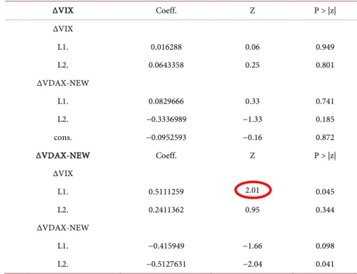
The VAR model results are reported in Table 3. In the first section, the VIX changes are examined with reference to their two lagged values and to the two lagged values of the VDAX-NEW changes. As the p-values suggest, none of the Table 2. Optimal lags number selection to include in the VAR model.
Lag LL LR df p FPE AIC HQIC SBIC
0 −435.178 219.65 11.0678 11.0918 11.1278*
1 −426.941 16.474 4 0.0002 197.323 10.9605 11.0326* 11.1405 2 −421.569 10.743* 4 0.030 190.641* 10.9258* 11.046 11.2257 3 −420.164 2.8103 4 0.590 203.706 10.9915 11.1597 11.4114 4 −419.22 1.8887 4 0.756 220.322 11.0689 11.2851 11.6087
6In the VAR models, each variable is explained as the evolution of its lags and the lags of the other
model variables.
7A time-series
t
Y is stationary if its joint probability distribution does not change when shifted in
time. The null hypothesis is that a unit root is present in the time-series. The alternative hypothesis is that the time-series is stationary.
8The choice of the autoregression order allows balancing the benefit to include a higher number of
lags with the cost of an increased estimate uncertainty.
9The LR test compares the goodness of fit of two models, one p order model and a p− order 1
model. The null hypothesis is that all the p lags are equal to zero. This test starts from the model
with the highest lags number, going on with the lower lags up to the rejection of the null hypothesis, this determining the best fitting lags number for the VAR model.
Table 3. VAR model between volatilities indexes and their lagged values. ΔVIX Coeff. Z P > |z| ΔVIX L1. 0.016288 0.06 0.949 L2. 0.0643358 0.25 0.801 ΔVDAX-NEW L1. 0.0829666 0.33 0.741 L2. −0.3336989 −1.33 0.185 cons. −0.0952593 −0.16 0.872 ΔVDAX-NEW Coeff. Z P > |z| ΔVIX L1. 0.5111259 2.01 0.045 L2. 0.2411362 0.95 0.344 ΔVDAX-NEW L1. −0.415949 −1.66 0.098 L2. −0.5127631 −2.04 0.041
lagged values seem to be significant for the VIX dynamic. In the second section, the VDAX-NEW changes are examined in relation to their two lagged values and the two lagged values of the VIX changes. Results show two significant re-sults: the first one refers to the negative relationship between the VDAX-NEW variation at time t − 2 and the VDAX-NEW variation at time t; the second, even more significant for the purposes of this study, is the positive relationship be-tween the VIX variation at time t − 1 and the VDAX-NEW variation at time t.
In order to identify a causality relationship between the two indexes, so, to determine whether the past values of one index is effective in forecasting the other, a Granger causality Test11 was performed (see Table 4). Table 4 reported,
for the current values of the VAR model variables (volatility index at the current time) and with reference to the VAR lagged variables (past values of the two in-dexes, tested by means of the F-Test), the results of the chi2 test and the p-values of the Wald test12.
The results in Table 4 show that in no case the p-value is great enough to re-ject the null hypothesis, so no index is useful to predict the other one.
Anyway, the joint consideration of the VAR model and the Granger causality test results suggest the existence of a linkage between the VIX at time t − 1 and VDAX-NEW at time t, even if no predictive power of one index on the other one is proofed.
As a last step of this first part of the analysis, we tested for the two indexes 11A variable X is said to Granger-cause Y if its lagged values have some predictive power on the
fu-ture values of Y. The null hypothesis is that the lagged values of X have not a predicting power for Y; the alternative hypothesis is that there is a Granger-causality.
12The Wald Test verify, through F-statistic, if some or all the lagged values of a variable are jointly
Table 4. Granger-causality Test on volatility indexes.
Equation Excluded chi2 df Prob > chi2
ΔVIXt ΔVDAX-NEW
(
t−1;t−2)
2.6632 2 0.264 ΔVIXt ΔVIX(
t−1;t−2)
2.6632 2 0.264 ΔVDAX-NEWt(
t−ΔVIX 1;t−2)
4.059 2 0.131 ΔVDAX-NEWt ΔVDAX-NEW(
t−1;t−2)
4.059 2 0.131Figure 2. Impulse Response Function ΔVDAX-NEW - ΔVIX.
Figure 3. Impulse Response Function ΔVIX - ΔVDAX-NEW.
linkages, by means of the Impulse Response Functions (IRF). These functions allow us to observe, for a specific time period (x-axis), the effect that a one stan-dard deviation shock on one index produces on the other index (in % on the vertical axis). After checking for the base hypotheses (uncorrelated and white noise error terms), we computed the Impulse Responses Functions between ΔVIX and ΔVDAX-NEW (Figure 2 and Figure 3).
As Figure 2 shows, the shock on the German volatility index causes no signif-icant reactions on the US volatility index.
On the other hand, Figure 3 shows that a US volatility index shock causes a significant reaction on the German volatility index.
The VAR model results, the graphical analysis of the IRFs and the past litera-ture13 support the hypothesis that the German volatility dynamic could be
influ-enced by the US volatility dynamic.
Starting from these results, in the second part of this study we examined the possible links between the macro “surprise effects” and the volatility indexes, by means of the following equations:
0 1 1 10 10
10
0 1
VIX Surprise Effect US Surprise Effect US Surprise EffectUS t t t t i it t i β β β β = β ∆ = + + + + = +
∑
+ (1) 6 0 1VDAX NEWt VIXt i Surprise Effect GERit t
i
β = β
∆ = ∆ + +
∑
+ (2)where:
1
VIXt VIXt VIXt−
∆ = − ;
1
VDAX NEWt=VDAX NEWt−VDAX NEWt− ;
0
β is the intercept;
i
β is the slope of the i-th surprise effect; t
is the error term.
The inclusion of ∆VIXt in Equation (2) allows the explicit consideration of the influence that the US volatility has on the German one, as seen in the pre-estimation analysis.
In order to correctly specify the econometric models, we tested the hypothesis of non-stationary of the time-series, by means of the ADF test, for the two con-sidered sub-periods14, and used the first differences, in order to make them
sta-tionary, for the time-series presenting a unit root, I(1).
5. Empirical Evidence of “Surprise Effects”
on Implied Volatility
This section presents the empirical results of the econometric estimations on each of the two time periods, January 2008-May 2012 (Table 5 and Table 6) and June 2012-December 2014 (Table 7 and Table 8). The tables report for each “macro surprise effects”, the regression coefficients, and its t-statistics and p-value. For each regression we also reported the F-statistic, its corresponding p-value (Prob > F) and the R2 coefficient.
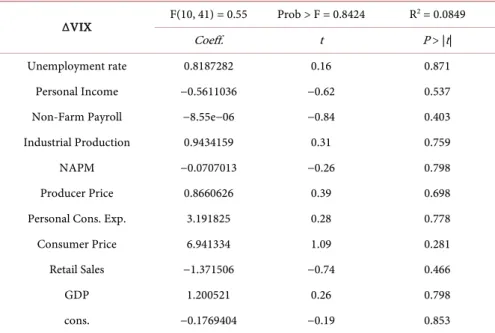
Table 6 presents the results of the joint and the marginal significance of Equ-ation (1) for the first time period, which checks for any relEqu-ationship between the “surprise effects” of the US indicators and its domestic market variability, meas-ured by the VIX index changes.
13[1][4][14][15][16][17][18] show the US economy relevance and the operators’ attention for
macro indicators.
14The ADF Test results for the first sub-period, show that the US GDP, the German GDP and the
IFO Business Climate Index are non-stationary; for the second sub-period, the US GDP and the German GDP are non-stationary.
599
Table 5. Links between the US indicators “surprise effects” and the VIX changes (Jan
2008-May 2012). ΔVIX F(10, 41) = 0.55 Prob > F = 0.8424 R 2 = 0.0849 Coeff. t P > |t| Unemployment rate 0.8187282 0.16 0.871 Personal Income −0.5611036 −0.62 0.537
Non-Farm Payroll −8.55e−06 −0.84 0.403
Industrial Production 0.9434159 0.31 0.759
NAPM −0.0707013 −0.26 0.798
Producer Price 0.8660626 0.39 0.698
Personal Cons. Exp. 3.191825 0.28 0.778
Consumer Price 6.941334 1.09 0.281
Retail Sales −1.371506 −0.74 0.466
GDP 1.200521 0.26 0.798
cons. −0.1769404 −0.19 0.853
Table 6. Links between the German indicators “surprise effects” and the VDAX-NEW
changes (Jan 2008-May 2012).
ΔVDAX-NEW F (7, 44) =14.22 Prob > F = 0.0000 R
2 = 0.8544
Coeff. t P > |t|
ΔVIX15 0.928709 8.52 0.000
Unemployment rate −0.1410833 −0.04 0.964
IFO Business Climate Index 0.7597552 3.20*** 0.003
Retail Sales −0.208779 −0.81 0.425
Producer Price 0.7155088 0.87 0.388
Industrial Production 0.2359803 0.84 0.407
GDP −0.2481186 −0.39 0.698
cons. 0.1233875 0.27 0.789
Results (t-statistics and p-values) show that no macro “surprise effect” of the US indicators has a significant influence on its domestic VIX index dynamics. The F-statistic value and the corresponding p-value do not allow rejecting the null hypothesis for the whole regression. This evidence and the low value of the R2 show the inability of the macro indicators to explain the volatility changes.
These findings are not surprising, as in that time period the markets ongoing was deeply influenced by the financial crisis, and the economic variables only had a minor influence on it.
Table 6 presents the results of the joint and the marginal significance of Equ-ation (2) for the first time period, so checking for any relEqu-ationship between the “surprise effects” of the German indicators and its domestic variability, meas-15Also ΔVIX coefficient is significant. As previously seen, the inclusion of ΔVIX allow considering
ured by the VDAX-NEW index changes.
The “surprise effect” of the IFO Business Climate Index16 is the only
signifi-cant variable, but at a 99% confidence level. This suggests a direct17 link between
the IFO surprise effect and the VDAX-NEW index dynamic. Also, the F-statistic value and its p-value allow rejecting the null hypothesis that all regression coef-ficients are zero, and the R2 value of 0.85 gives evidence to the importance of this
effect.
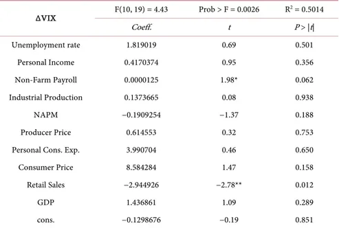
Table 7 presents the results of the joint and the marginal significance of Equ-ation (1) for the second time period, checking for any relEqu-ationship between the “surprise effects” of the US indicators and the VIX index changes.
The lower volatility characterizing the second time period allow for the eco-nomic effects to be evidenced by the model. Results show that the significant “surprise effects”, for the VIX index dynamic, are related to18 Non-Farm Payroll,
with a 10% significance level, and Retail Sales, with a 5% significance level. In particular, the coefficients signs show a direct relation between the surprise ef-fect of the Non-Farm Payroll and the VIX index changes, and an inverse relation between the surprise effect of the Retail Sales and the VIX index changes.
Unlike the results of equation (1) for the first time period, the null hypothesis is rejected, and the R2 value reports that the model explains nearly half of the
variations.
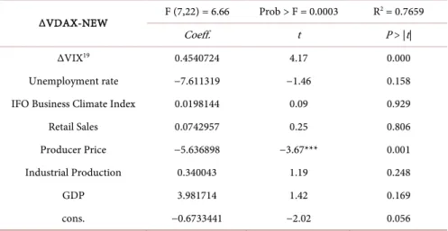
Table 8 presents the results of the joint and the marginal significance of Equ-ation (2) for the second time period, checking for any relEqu-ationship between the “surprise effects” of the German indicators and the VDAX-NEW index changes.
Table 7. Links between the US indicators “surprise effects” and the VIX changes (Jun
2012-Dec 2014). ΔVIX F(10, 19) = 4.43 Prob > F = 0.0026 R 2 = 0.5014 Coeff. t P > |t| Unemployment rate 1.819019 0.69 0.501 Personal Income 0.4170374 0.95 0.356 Non-Farm Payroll 0.0000125 1.98* 0.062 Industrial Production 0.1373665 0.08 0.938 NAPM −0.1909254 −1.37 0.188 Producer Price 0.614553 0.32 0.753
Personal Cons. Exp. 3.990704 0.46 0.650
Consumer Price 8.584284 1.47 0.158
Retail Sales −2.944926 −2.78** 0.012
GDP 1.436861 1.09 0.289
cons. −0.1298676 −0.19 0.851
16Also [1] found similar results.
17The coefficient sign represents the link between the surprise effect and the volatility index changes.
A direct link (positive sign) means that a positive or negative “surprise effect” influences positively or negatively the volatility changes.
601
Table 8. Links between the German indicators “surprise effects” and the VDAX-NEW
changes (Jun 2012-Dec 2014).
ΔVDAX-NEW F (7,22) = 6.66 Prob > F = 0.0003 R
2 = 0.7659
Coeff. t P > |t|
ΔVIX19 0.4540724 4.17 0.000
Unemployment rate −7.611319 −1.46 0.158
IFO Business Climate Index 0.0198144 0.09 0.929
Retail Sales 0.0742957 0.25 0.806
Producer Price −5.636898 −3.67*** 0.001
Industrial Production 0.340043 1.19 0.248
GDP 3.981714 1.42 0.169
cons. −0.6733441 −2.02 0.056
The estimation results show that the “surprise effect” of the Producer Price Index is the only significant variable, with a 99% confidence level, with a nega-tive value declaring an inverse link between the Producer Price surprise effect and the VDAX-NEW index dynamic. Here also, the null hypothesis is rejected, and the R2 value of 0.76, proof an important explanatory power of the model.
6. Conclusions and Remarks
This study analyzed the possible links between the “surprise effect” of some ma-cro indicators news and the dynamic of the US and the German volatility in- dexes.
The preliminary tests on the possible relationship between the VIX and the VDAX-NEW indexes, show that the US volatility has a positive influence on the German one, but not vice versa.
The analysis separately performed on the two time periods from January 2008 to May 2012 and from June 2012 to December 2014 shows that for the first time period, whose financial environment was highly volatile, no links between the US “surprise effect” and the VIX index changes are significant. Instead, the German market analysis shows a direct link between the “surprise effect” of the IFO Business Climate Index and the VDAX-NEW index changes.
With reference to the second time period (June 2012-December 2014), cha-racterized by moderate and relatively flat volatility, some significant macro “surprise effects” for the volatility indexes were found, specifically related to the industrial sector (US Retail Sales, German Producer Price) and the job market (US Non-Farm Payroll).
The empirical findings and a careful analysis of the possible “surprise effect” coefficients can actually support the market operators to take timely positions (long or short) on the derivatives markets, based on the expected volatility dy-namic, using specific derivatives instruments (especially options) on the VIX and VDAX-NEW indexes, for improving the investment and hedging strategies. 19See supra note 15.
Evidently, the different news, more and more frequent and incomplete, needs a careful analysis, because its fragmentation increases the market uncertainty. But even if this kind of news, in fact, when not completed by other information, does not allow having an overall and rational picture of the actual economic framework, nonetheless can be an important information source when used for short-term speculative or hedging purposes.
These results also suggest some possible extensions. The actual European eco- nomic context, characterized by the Governments’ instability, possibly due to their intense political calendars, and inducing financial markets’ uncertainty, has enhanced the leadership of Germany within the Eurozone. Thus, it would be in-teresting to extend the same research approach to test for the actual role of Ger-many with reference to the other Eurozone countries, and to verify if the same effects on the other countries are mainly related to Germany, to the US, or to other countries’ determinants.
References
[1] Funke, N. and Matsuda, A. (2002) Macroeconomic News and Stock Returns in the United States and Germany. IMF Working Paper, WP/02/239.
[2] Nikkinen, J. and Sahlström, P. (2003) Scheduled Domestic and US Macroeconomic News and Stock Valuation in Europe. Journal of Multinational Financial Manage-ment, 14, 201-215.
[3] Nikkinen, J. and Sahlström, P. (2004) Impact of the Federal Open Committee Meetings and Scheduled Macroeconomic News on Stock Market Uncertainty. In-ternational Review of Financial Analysis, 13, 1-12.
[4] Nikkinen, J., Omran, M., Sahlström, P. and Äijö, J. (2006) Global Stock Market Reaction to Scheduled U.S. Macroeconomic News Announcements. Global Finance Journal, 17, 92-104.
[5] Nofsinger, J.R. and Prucyk, B. (2003) Option Volume and Volatility Response to Scheduled Economic News Releases. The Journal of Futures Markets, 23, 315-345. https://doi.org/10.1002/fut.10064
[6] Schwert, W.G. (1989) Why Does Stock Market Volatility Change Over Time? The Journal of Finance, 44, 1115-1153.
https://doi.org/10.1111/j.1540-6261.1989.tb02647.x
[7] Bomfim, A.N. (2003) Pre-Announcement Effects, News Effects, and Volatility: Monetary Policy and the Stock Market. Journal of Banking and Finance, 27, 133- 151.
[8] Gümüş, G.K., Yücel, A.T., Karaoǧlan, D. and Çelik, S. (2011) The Impact of Do-mestic and Foreign Macroeconomic News on Stock Market Volatility: Istanbul Stock Exchange. Bogazici Journal, 25, 123-137.
[9] Merton, R.C. (1973) The Theory of Rational Option Pricing. The Bell Journal of Economics and Management, 4, 141-183.https://doi.org/10.2307/3003143
[10] Donders, M.W.M. and Vorst, T.C.F. (1996) The Impact of Firm Specific News on Implied Volatilities. Journal of Banking and Finance, 20, 1447-1461.
[11] Kearney, A.A. and Lombra, R.E. (2004) Stock Market Volatility, the News, and Monetary Policy. Journal of Economic and Finance, 28, 252-259.
https://doi.org/10.1007/BF02761615
Announcements. Finance Research Letters, 4, 227-232.
[13] Lee, Y.H., Hung, J.C., Wang, Y.H. and Huang, C.Y. (2012) A Study of Dynamics in Market Volatility Indices between the US and Taiwan. Investment Management and Financial Innovations, 9, 89-95.
[14] Belgacem, A. (2008) Fundamentals, Macroeconomic Announcement and Asset Prices. University of Paris Ouest-Nanterre La Défense and CNRS, Paris.
[15] Bollerslev, T., Cai, J. and Song, F. (2000) Intraday Periodicity, Long Memory Vola-tility, and Macroeconomic Announcement Effects in the US Treasury Bond Market. Journal of Empirical Finance, 7, 37-55.
[16] Dimpfl, T. (2011) The Impact of US News on the German Stock Market—An Event Study Analysis. Quarterly Review of Economic and Finance, 51, 389-398.
[17] Graham, M. and Sahlström, N.J. (2003) Relative Importance of Scheduled Macroe-conomic News for Stock Market Investors. Journal of Economics and Finance, 27, 153-165.https://doi.org/10.1007/BF02827216
[18] McQueen, G. and Roley, V.V. (1993) Stock Prices, News, and Business Conditions. The Review of Financial Studies, 6, 683-707.https://doi.org/10.1093/rfs/5.3.683
Submit or recommend next manuscript to SCIRP and we will provide best service for you:
Accepting pre-submission inquiries through Email, Facebook, LinkedIn, Twitter, etc. A wide selection of journals (inclusive of 9 subjects, more than 200 journals)
Providing 24-hour high-quality service User-friendly online submission system Fair and swift peer-review system
Efficient typesetting and proofreading procedure
Display of the result of downloads and visits, as well as the number of cited articles Maximum dissemination of your research work
Submit your manuscript at: http://papersubmission.scirp.org/ Or contact [email protected]