Dipartimento di Fisica e Astronomia
Dottorato di Ricerca in Fisica - XXIII Ciclo
AN OBSERVATIONAL AND
THEORETICAL STUDY OF THE
MAGNETIC HELICITY FLUX
Author
Aimilia Smyrli
Coordinator:
Supervisors:
Prof. Francesco Riggi
Prof. Francesca Zuccarello
Dr. Duncan Mackay
Co-supervisor:
The study of magnetic helicity started in 1969 when Moffatt (Moffatt 1969) emphasized the necessity of introducing an invariant into Euler’s equations, that can provide a bridge between topology and fluid dynamics. This quantity was determined to be magnetic he-licity, that can measure the complex geometry and the mixing properties of a magnetic field such as the twist, braiding or linkage of the field lines during different phases of its evolution.
Not surprisingly, the solar physicists community is attracted by this physical parame-ter, that amongst others has the remarkable property to remain approximately conserved in a perfectly conducting plasma (with high magnetic Reynolds number, as proposed by Taylor (1974) or Berger & Field (1984)). For example, the conservation of magnetic he-licity in the solar convective zone can provide significant information on the alpha effect in solar dynamo theory. Nevertheless, what is actually interesting is that helicity may be used to understand dynamic processes such as Coronal Mass Ejections (CMEs), flares and filament eruption, that lead to the large amounts of energy release and so avoid an endless storage of magnetic helicity in the solar corona. Hence, the observational study of magnetic helicity has received considerable attention since it carries information about the structure of the magnetic field configuration and the conditions under which this structure can lead to an instability that acts as a precursor for an eruptive event.
In this thesis, magnetic helicity is investigated both observationally and theoretically. In the first Chapter we introduce some important concepts used in our investigations, such as the basic characteristics of CME events and the magnetic helicity definition and its application to solar phenomena.
of halo CMEs. This is a first step aimed at providing a solution to some hotly debated questions related to CMEs, such as “Which, when, how and why?” an active region can reach the configuration necessary to trigger the explosion of a CME. Initially, we focus on identifying the active regions (ARs) that are suspected to be probable CME initiation sites. This is achieved by making use of sequential full-disk solar images from the Extreme Ultraviolet Imaging Telescope (EIT) onboard the space-borne Solar and Heliospheric Ob-servatory (SOHO) and by computing the difference between successive images in all the wavelengths, with the pivot image the one being closest to the occurrence of the CME. An important difference in brightness together with the indication of a flare or a filament eruption allows us to select the AR where the CME was initiated.
In this way we limit our analysis to 10 ARs. The only chance to investigate the evolution of magnetic helicity, can be provided by the analysis of magnetic fields. Thus, we work with data obtained from the Michelson Doppler Imager (MDI) magnetograph onboard the SOHO satellite. The Local Correlation Tracking (LCT) method is applied in order to obtain the horizontal velocities and a Fast Fourier Transform (FFT) method is used in order to get the vector potential.
We find that the magnetic helicity injection does not have a unique trend in the events analyzed: in 40 % of the cases it shows a large sudden and abrupt change that is temporally correlated with a CME occurrence, while in the other cases it shows a steady monotonic trend, with a slight change in magnetic helicity at CME occurrence (Smyrli et al., 2010). However, a key result concerns the active regions where both X-class flares and CMEs occur. In these cases major changes in the magnetic helicity flux take place prior to the CME detection and are connected to an increase in the magnetic flux. This means that the emergence of magnetic flux from subphotospheric layers can change significantly the active region magnetic configuration, by shearing or twisting, and so trigger instabilities that will eventually lead to eruptive events. Consequently, the study of the motion of magnetic concentrations occurring in the convective supergranular cells, their
In the third Chapter, we consider the small scale build up of magnetic helicity in a convective supergranular cell. We study the motion of magnetic features (bipoles) in a convective cell that is simplified into the form of a hexagonal cell, with a diameter of ∼ 40 arcsec, or ∼ 30, 000 km. As a first step, we work with one bipole and then with more to a maximum number of five. Different processes are studied between polarities of opposite sign such as cancellation, emergence, advection (’fly-by’), coalescence or fragmentation, depending on the initial tilt angle of the inserted bipole. In order to study the effects of different magnetic fragment motions in the supergranular cell into the magnetic helicity accumulation, we apply the same code that we have already used in the Chapter 2 for the observational data analysis.
Our results show that a short distance between magnetic fragments, and thus strong relative motions, can be a key element in the accumulation of large amounts of magnetic helicity. This can be the case of new emergence of new polarities or the case where two polarities are passing by each other (“fly-by”), but without any interaction. More impor-tantly, we notice the highest production of magnetic helicity in neighboring borders of the supergranular cell, something that can indicate the occurrence of eruptive events in the corona above these “junction” points. In contrast, when no shearing is observed, i.e when the initial tilt angle is ±90◦, the accumulated helicity is very small.
The results obtained in this research, using both the observational and the theoretical approach, motivate future investigations that are briefly described in the last Chapter.
Abstract V
1 Introduction 1
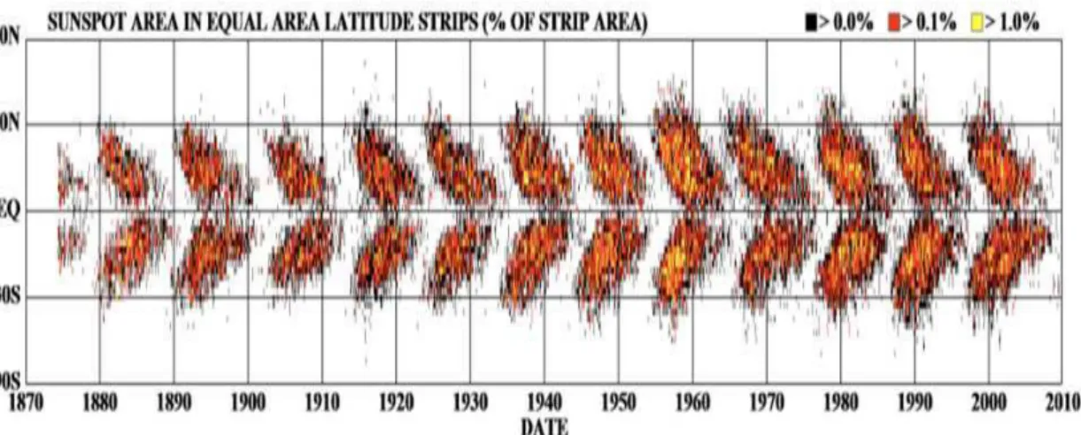
1.1 The Butterfly Diagram and the Solar Activity . . . 3
1.2 Coronal Mass Ejections . . . 4
1.2.1 Observing Techniques . . . 5
1.2.2 CME basic characteristic properties . . . 5
1.2.3 CME Theoretical Models . . . 9
1.2.4 Mini-CMEs . . . 10
1.3 Magnetic Helicity . . . 11
1.4 Thesis Outline . . . 14
2 Origin Sites of CMEs and Magnetic Helicity 17 2.1 Motivation . . . 18
2.2 Analysis of EIT images . . . 25
2.3 Analysis and Selection of MDI images . . . 35
2.3.1 Magnetic Helicity Calculation in the coronal volume of an active region . . . 35
2.3.2 Magnetic Helicity from MDI data . . . 37
2.4 Results . . . 41
2.4.1 Class I: Gradual CMEs . . . 41
2.5 Discussion . . . 51
2.6 Future Work . . . 54
3 Magnetic Helicity Inside a Convective Cell 57 3.1 Introduction . . . 58
3.2 Model Set Up . . . 63
3.3 Test Cases . . . 68
3.3.1 Application of the code of Chae . . . 68
3.3.2 Study of different motions of a bipolar pair . . . 73
3.3.3 Summary of the Results . . . 86
3.4 SINGLE BIPOLE INSIDE A HEXAGONAL CELL . . . 88
3.4.1 “FLY-BY” ALONG THE HEXAGONAL SIDES . . . 91
3.4.2 CANCELLATION ON A HEXAGONAL VERTEX . . . 93
3.4.3 WHEN THE NEGATIVE POLARITY ENDS AT V4 AND A CASE OF EMERGENCE . . . 98
3.4.4 WHEN THE NEGATIVE POLARITY ENDS AT THE V3 . . . 102
3.4.5 WHEN THE NEGATIVE POLARITY ENDS AT THE V2 . . . 106
3.4.6 WHEN THE NEGATIVE POLARITY ENDS AT V1. . . 109
3.4.7 WHEN THE NEGATIVE POLARITY ENDS AT V6. . . 111
3.5 DISCUSSION OF THE SIMPLE BIPOLE CASE . . . 115
3.6 RANDOM GENERATION OF BIPOLES INSIDE A HEXAGONAL CELL 117 3.7 DISCUSSIONS ON THE MOTION OF MULTIPLE BIPOLES INSIDE A HEXAGONAL CELL . . . 119
4 Conclusions and Future Work 123 4.1 Conclusions . . . 123
4.2 Future Work . . . 126
1.1 Structure of the Sun . . . 2
1.2 The Sunspot Butterfly Diagram . . . 4
1.3 CME, dimming and flare events on 12/05/1997 . . . 6
1.4 Three-part Structure of a CME . . . 7
1.5 Patterns with positive magnetic helicity . . . 13
2.1 Full-disk AIA/SDO images at the wavelength of 171 ˚A during the morning of 01/08/2010 . . . 20
2.2 Magnetic cloud drawing . . . 23
2.3 A halo CME observed by LASCO/C2 and EIT . . . 26
2.4 The EIT instrument . . . 26
2.5 Full-disk EIT images at 171 ˚A, 195 ˚A, 284 ˚A and 304 ˚A . . . 27
2.6 Difference of full-disk 171 ˚A and 284 ˚A EIT images for the halo CMEs that occurred on 15/07/2002 and on 16/08/2002 respectively . . . 29
2.7 Selection of active regions in a full-disk 171 ˚A difference image related to the CME event of 09/11/2002 . . . 30
2.8 Difference images of 171 ˚A for NOAA 10030 on 16/07/2002 . . . 30
2.9 Plotted size and intensity of the NOAA 10030 for the halo CME event on 16/07/2002 . . . 32
2.10 Table1 . . . 34
2.12 Zoom of NOAA 10030 for an EIT/SOHO image and a MDI/SOHO
mag-netogram . . . 36
2.13 Schematic drawing of a flux tube that rises through the photosphere . . . . 38
2.14 Plotted Results for NOAA 8858 & NOAA 9415 . . . 43
2.15 Same as in Figure 2.14 for ARs 8948, 9114+9115 and 9393+9394, belong-ing to Class I (gradual CMEs). . . 45
2.16 Same as in Figure 2.14 for ARs 10030 and 10069+10077, belonging to Class II (impulsive CMEs). . . 47
2.17 Same as in Figure 2.14 for ARs 10162, 10229 and 10365, belonging to Class II (impulsive CMEs). . . 50
2.18 Table2: Characteristics of the active regions, halo CMEs and analyzed rel-evant eruptive events. . . 51
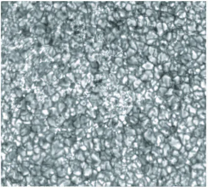
3.1 Solar Granulation image taken with the Swedish Solar Telescope . . . 59
3.2 Sketch of the horizontal motions at the top of a supergranule . . . 60
3.3 Magnetic Bright Points located in intergranular lanes . . . 61
3.4 “Magnetic Carpet” . . . 63
3.5 A Hexagonal Cell with length L . . . 65
3.6 (a)The hexagonal cell, the smaller boc and the bipoles (b)Gaussian profile for the magnetic field . . . 67
3.7 Gaussian profile of magnetic field for the “fly-by” process . . . 71
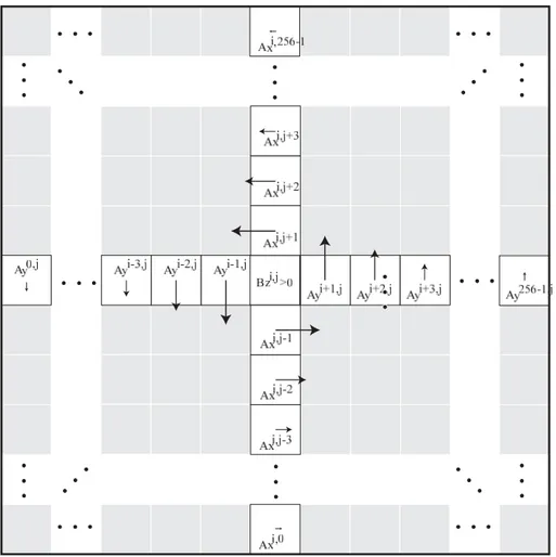
3.8 Evolution of Ax and Ay along the y and x direction for a positive polarity that is located in the (xi, yi) inside the whole computational domain . . . . 73
3.9 Surface plots of the Ax and Ay component of the vector potential for the positive and the negative polarities for the first snapshot in the “fly-by” process . . . 74
3.10 spatial evolution of Ay and Ax along the x and y axis for the positive and negative polarities . . . 75
3.12 “Fly-by” case: plotted Hi, Φ and dH/dt for (x1, y1) = (0.25, 0.25) and
(x2, y2) = (0.75, 0.75) and (x1, y1) = (0.25, 0.30) and (x2, y2) = (0.75, 0.70) . 78
3.13 Same as in Figure 3.11 for (x1, y1) = (0.25, 0.35) and (x2, y2) = (0.75, 0.65)
and (x1, y1) = (0.25, 0.40) and (x2, y2) = (0.70, 0.60) . . . 79
3.14 Same as in Figure 3.12 but now (x1, y1) = (0.25, 0.40) and the negative on
(x2, y2) = (0.75, 0.55) . . . 80
3.15 Cancellation between two opposite polarities . . . 81 3.16 Hi,Φ and dH/dt for the cancellation process a) along the x-axis and b)at
an angle . . . 83 3.17 Hi,Φ and dH/dt for the case of emergence . . . 84
3.18 Coalescence of two positive polarities . . . 85 3.19 Fragmentation for a initially large positive polarity into two smaller . . . 87 3.20 The six equilateral triangles that compose a hexagonal cell . . . 89 3.21 Snapshot for the motion inside a hexagonal cell with initial tilt angle 90◦
. 92 3.22 Plots that show the evolution for magnetic helicity accumulation (Hi, Hi+,
Hi−), rate of transport of magnetic helicity (dH/dt, dH/dt+, dH/dt−) and
total absolute magnetic flux (|Φ|) . . . 94 3.23 Same parameters as in Figure 3.22. Case where the positive polarity ends
on V5 and the negative on V1 . . . 95
3.24 Snapshots for a cancellation case on the vertex V5 . . . 95
3.25 Same parameters as in Figure 3.22. Case of cancellation where both po-larities end on V5 . . . 97
3.26 Snapshots for another cancellation case . . . 97 3.27 Same parameters as in Figure 3.22. Another case of cancellation where
both polarities end on V5 . . . 99
3.28 Snapshots for the case that the negative polarity ends at V4and the positive
at V5 . . . 99
3.29 Same parameters as in Figure 3.22. A case of initial emergence. The neg-ative polarity ends at V4 and the positive at V5 . . . 101
3.30 Snapshots of the case that the negative polarity ends at V4and the positive
at V5 . . . 101
3.31 Same parameters as in Figure 3.22. Another case where the negative polarity ends at V4 and the positive at V5 . . . 103
3.32 Snapshots for the case that the negative polarity ends at V3and the positive
at V5 . . . 103
3.33 Same parameters as in Figure 3.22. A case where the negative polarity ends at V3 and the positive at V5 . . . 105
3.34 Snapshots of the case that the negative polarity ends at V3and the positive
at V5 . . . 105
3.35 Same parameters as in Figure 3.22. Another case where the negative polarity ends at V3 and the positive at V5 . . . 106
3.36 Snapshots of the case that the negative polarity ends at V2and the positive
at V5 . . . 107
3.37 Same parameters as in Figure 3.22. A case where the negative polarity ends at V2 and the positive at V5 . . . 108
3.38 Snapshots of the case that the negative polarity ends at V1and the positive
at V5 . . . 109
3.39 Same parameters as in Figure 3.22. A case where the negative polarity ends at V1 and the positive at V5 . . . 110
3.40 Snapshots of the case that the negative polarity ends at V6and the positive
at V5 . . . 111
3.41 Same parameters as in Figure 3.22. A case where the negative polarity ends at V6 and the positive at V5 . . . 112
3.42 Snapshots for another the case that the negative polarity ends at V6 and
the positive at V5 . . . 113
3.43 Same parameters as in Figure 3.22. Another case where the negative polarity ends at V6 and the positive at V5 . . . 114
3.44 Random generation of two, three and four bipoles: snapshots and total magnetic helicity accumulation . . . 121 3.45 Random generation of five bipoles with different “sheed” number: snapshots
Introduction
“Always keep Ithaca in your mind. To arrive there is your ultimate goal...” Konstantinos P. Kavafis, “Ithaca” (1911)
The actual heart of the solar system that sustains the necessary energy for the existence of life on Earth is the Sun. Thus, is not surprising that the study of our closest star has attracted the interest of hundreds of scientists. Moreover, the Sun is interesting as an astrophysical laboratory and since it is the nearest star and can be studied in much greater detail than others, we can use the obtained information to explain many astrophysical processes that occur in other stars, or planets or in general in the Universe.
The Sun is classified as a G2 V star. The mass of the Sun is composed of about 70% hydrogen, 28% helium and the rest of other heavier elements (such as oxygen, carbon, neon, magnesium etc.). It has a mass of 1.99 × 1030 kg, luminosity 3.85 × 1026 W, and radius 6.96 × 10⁸ m. The Sun and its extended atmosphere can be divided in a number
of layers, as shown in Figure 1.1, according to the physical processes that are responsible for the generation and transport of energy in each region. The solar interior whose main characteristics have been confirmed by helioseismology can be divided as follows:
• The Core is the central region in the solar interior that covers ∼ 20 − 25% of the solar radius. Here, thermo-nuclear reactions take place from which the solar energy
Figure 1.1: Schematic drawing of the structure of the Sun illustrating the dif-ferent internal and atmospheric layers.Image courtesy from McREL (http :
//genesismission.jpl.nasa.gov/science/mod3SunlightSolarHeat/SolarStructure/index.html).
flux is generated
• The Radiative Zone covers the region between 0.25 and 0.7 R⊙. The transfer of
energy, that is generated in the core, through the radiative zone can be approximated by a process of interaction between radiation and matter.
• The Tachocline is the thin layer between the radiative and the convective zone where the fluid flow velocities change, i.e from almost rigid to differential rotation.
• The Convective Zone extends from 0.7 R⊙ up to the visible surface. Convective
motions transfer heat rapidly to the surface
The dividing layer between the solar interior and the solar atmosphere is the photo-sphere, the visible surface. Above the photosphere lies the solar atmosphere that consists of the chromosphere, the transition region, the corona and the heliosphere.
In this thesis we focus on processes that take place both in the solar interior (more specifically in the convective zone) and in the solar atmosphere (more specifically dynamic
phenomena such as CMEs, flares and filament eruptions). Our aim is to understand how the interactions between fluid flows and magnetic fields can lead to complex magnetic configurations that can trigger eruptive events.
1.1
The Butterfly Diagram and the Solar Activity
In 1609 Galileo Galilei constructed the first telescope, he turned it to the Sun and charted the location and number of sunspots. Historically, the sunspot observation has provided the most important constraint of the solar activity: a continuously changing magnetic field which however shows periodicity: Plotting the location of sunspots versus the time reveals the so-called butterfly diagram, where two latitude bands on either side of the solar equator appear and first form at mid-latitudes and then move towards the equator as each cycle evolves (see Figure 1.2). Each cycle lasts around 11 years. Since sunspots are man-ifestations of strong magnetic fields (that can reach up to ±3000 G), this cycle provides information about the solar magnetic activity. Moreover, sunspots occur in bipolar pairs consisting of a leading and a trailing spot of opposite polarity and according to Hale’s Law the polarities are reversed in the two hemispheres and reverse in successive solar cy-cles. This means that every 22 years a hemisphere will be characterised by sunspot pairs of the same sign. Hence, the period of the Sun’s magnetic cycle is about 22 years. Addi-tionally, the line joining the leading and the trailing spots is inclined at an angle of ∼ 4◦
to the equator with the leading polarity being close to the equator and the trailing one close to the poles (Joy’s Law). For a detailed study of the solar activity see the review of Usoskin (2008) and references therein.
The 22-year activity is considered to be a manifestation of the dynamo action that takes place in the solar interior, in the tachocline. There are two main driver mechanisms for the solar dynamo :
1. the solar differential rotation that produces a toroidal magnetic field from an already existing poloidal field
Figure 1.2: The Sunspot Butterfly Diagram derived by the solar group at NASA Marshall Space Flight Centre.
in the convective zone and lead to the production of a large-scale poloidal field from a mean toroidal field. The action of the Coriolis force on the convective vortices results in right-handed vortices in the Northern solar hemisphere and left-handed vortices in the South. Thus, right and left helicities in each hemisphere give rise to the conversion of a toroidal field to a poloidal.
The solar magnetic field is considered to be the source of most solar active phenomena such as the three large-scale manifestations of the solar activity: the Coronal Mass Ejections (CMEs), the flares and the filament eruptions.
In the following, we will describe the main characteristics of CMEs, because most of the research carried out in this thesis deals with these phenomena.
1.2
Coronal Mass Ejections
Coronal Mass Ejections (CMEs) are sudden explosions of magnetized plasma clouds from the solar atmosphere into the interplanetary medium. These violent manifestations of the solar activity are considered to be responsible for Space Weather disturbances and when directed towards the Earth, also for geomagnetic storms (as discussed for example in Kosk-inen & Huttunen (2006)). In that case, we have to face major damages such as the failure
(temporal or even worse, permanent) of satellites, the exposure of astronauts to radiation or the disruption of communication and navigation power systems (e.g on 13/03/1989 the city of Quebec lost half of its electrical power generation due to a large CME eruption). That is the reason why the study and prediction of CME events is considered as essential by the solar physicists community. Since the detection of the first CME on 14/12/1971 (Tousey (1973)) by the space based coronograph on board the Orbiting Solar Observatory 7 (OSO-7), million of CME events have been detected, studied and carefully analyzed.
1.2.1 Observing Techniques
CMEs are mainly observed with the help of coronographs. Coronographs observe the Thomson-scattered light by electrons and so CMEs appear as two-dimensional white-light features projected on the plane of the sky. Nevertheless, we know that most of the production and development of a CME takes place lower in the corona, below the occulting disk of a coronograph. Observations in different wavelenghts have revealed the coronal restructuring that underlies a CME event and various phenomena that can be connected to them, i.e. the coronal or EUV dimmings (Sterling & Hudson (1997)), soft X-ray sigmoid structures (Canfield et al. (1999)), EIT waves (Thompson et al. (1998)), filaments observed in Ha, or type II radio bursts (Wild & McCready (1950)) that reveal
MHD shock waves propagating away from coronal disturbances such as CMEs and flares. In Figure 1.3 we present the eruptive event of 12/05/1997 where a CME, a flare, dimming and associated EIT wave where observed (the event is presented in Attrill et al. (2006) ).
1.2.2 CME basic characteristic properties
The basic features of the CMEs that have been obtained through statistical studies of various datasets can be summarized as follows:
∗ Morphology. Traditionally, observers with the help of coronograph white-light im-ages have defined a CME as a three-part structure that consists of a bright front loop overlying a coronal dark cavity that includes a bright core comprising prominence material (as was firstly detected in the prototypical CME event of
Figure 1.3: a) An EIT difference image showning the flare site, twin dimming regions and a propagating wave. The event was examined by Attrill et al. (2006) and the image is taken from van Driel-Gesztelyi & Culhane (2009).
18/08/1980 by Illing & Hundhausen (1985)) . Figure 1.4 shows an example of the three-part morphology of a CME as presented in Riley et al. (2008). Within the dark cavity there is a helical magnetic field structure that is connected to the presence of an expanding flux rope (as suggested for example from Cremades & Bothmer (2004) and Krall (2007) and was confirmed by stereoscopic observations from Th-ernisien et al. (2009) or Wood & Howard (2009)). The outermost bright leading edge is a dense plasma shell that is regarded as the material that has been swept up by the erupting flux rope and interacted with the ambient coronal plasma, i.e it is considered to be a shock driven by the flux rope ahead of the CME.
Since the inner bright core is observed to be emitting in the Haline, it is composed
of much cooler plasma which is assumed to originate from a prominence eruption that occurred below the field of view of the coronograph.
Figure 1.4: Three-part structure of a CME: bright leading edge, dark cavity and a bright central region that is called the core. The event was observed by LASCO on 27/02/200 at 07:42UT and is presented in Riley et al. (2008).
∗ Occurrence Rate. During the solar maximum we can observe daily around six (or even more) CMEs, whereas during the solar minimum the number of observed CMEs falls down to 0.5/day. Gopalswamy et al. (2003a) have studied the 23rd solar cycle and discovered individual cases where more than a dozen CMEs occurred in a day.
∗ Position Angle- Latitude Distribution. The projected angular centroid of a CME defines its apparent latitude and is strongly connected to the CME source region(Hundhausen (1993)). During the solar minimum the CMEs cluster at low latitudes (±10◦
around the equator), whereas during the solar maximum they appear at all latitudes(St. Cyr et al. (2000); Gopalswamy (2003)). However, we should note that there is no equatorward drift observed at low latitudes (Li et al. (2009)), and that the apparent latitudes of CMEs are more connected with the latitudes of helmet
streamers (St. Cyr et al. (2000)) than with the latitudes of active regions that the butterfly diagram reveals.
∗ Angular Width The angular width of a CME is measured as the position angle extent in the plane of the sky. According to their angular size the CMEs can be grouped in four classes (following the work presented by Mishra & Tripathi (2006) and Howard et al. (1982)) :
– narrow CMEs with an angular width smaller than 20◦
.
– normal CMEs with angular width in the range between 20◦
and 120◦
.
– wide CMEs with angular width higher than 120◦
.
– partial halo CMEs with 120◦
≤ angular width leq 360◦
.
– halo CMEs with angular size equal to 360◦
. We note that there can be different definitions of halo CMEs: for example Kim et al. (2005) defined as halo CMEs the events with angular width larger than 120◦
.
Halo CMEs are interpreted as the result of the Thompson scattering of Sun’s white light along the line-of-sight caused by a wide bubble (i.e shell) of dense plasma that is ejected in the frontside or backside of the Sun (Howard et al. (1982)). Halo CMEs are considered to be more geoeffective (i.e able to cause geomagnetic storms with intensity ≤ -50 nT) than the other CME events (stud-ies carried out on this topic can be found for example in Zhao & Webb (2003) and Gopalswamy et al. (2007))
As far as the solar cycle dependence is concerned, it has been detected an increase in the percentage of narrow and normal CMEs during the solar maximum( Mishra & Tripathi (2006)), and a decrease in the percentage of wide CMEs during the minimum phases of the solar cycle(St. Cyr et al. (2000)). It is possible that the angular width is subject to projection effect errors and for CMEs that are away from the solar limb, is overestimated. Interestingly, Moore et al. (2007) studied three CMEs originating from flare regions and showed that the final angular width that a CME has in the
outer corona can be directly connected to the average magnetic field strength and to the angular width of the flaring source region.
∗ Speed The speed of CMEs is defined by tracking their coronographig images in the plane of sky and so even in this case errors due to projection effects can occur. The speed of a CME can change within the coronographic field of view because it can be subject to propelling and retarding forces. CME speeds range from less than 20 km/s up to 3000 km/s. Halo CMEs are more energetic, their average speed is around 1000 km/s in comparison with the ordinary CMEs having velocities around 470 km/s. Moreover, CMEs related to active regions have higher average speeds than those connected to eruptive prominences located far from active regions (Gosling et al. (1976)).
∗ Acceleration The CME acceleration within the coronographic field of view is speed-dependent. Yashiro et al. (2004) found that the majority of the slow CMEs (i.e with velocities ≤ 250 km/s) show acceleration, indicating a continuous energy release, whereas the fast ones (with a speed higher than 900 km/s) show deceleration. More-over, CMEs that are moving at the solar wind speed show little acceleration. Mac-Queen & Fisher (1983) showed that CME events that are associated to flares have more rapid accelerations. On this basis, in Chapter 2 we will divide our sample of CME events into two categories : gradual and impulsive.
∗ Mass During a CME event between 1012g and 1016g of coronal material is ejected.
This mass is estimated from coronographic images taking into account the excess of brightness of a CME image relative to an image taken before the event. Hence, the mass that the occulting disk is covering cannot be included and the CME masses are in general underestimated due to the assumption that all of the CME material is located in the plane of the sky (Vourlidas et al. (2000)). The kinetic energy of a CME can be determined through the obtained masses and speeds and is between 1027 erg and 1033 erg. Vourlidas et al. (2002) proposed a power-law distribution to describe the masses and the kinetic energies of CMEs, in contrast with Jackson &
Howard (1993), who presented an exponential distribution.
1.2.3 CME Theoretical Models
Even though many of the properties of the CMEs are well known, their initiation remains still an unresolved problem (Forbes et al. (2006)). On the one hand, the current obser-vations do not always provide us information about the magnetic field configuration in the low corona, where the initial stages of the CME evolution occur. On the other hand, even though there is a variety of theoretical models that have been developed to explain the triggering mechanism and observed properties of CMEs, surprisingly, it has not yet been developed a single model that can describe all of the observational data and observed processes (in the lower levels of the atmosphere or in the solar wind) related even to a single CME event.
In the breakout model (Antiochos et al. (1999)) a quadrupolar flux distribution is con-sidered consisting of an overlying arcade whose flux is oppositely directed with respect to the underlying central arcade and two lateral flux systems. In this scenario the emergence of new magnetic flux (Zuccarello et al. (2008)) and/or the shearing motions along the magnetic inversion line eventually result in a CME. Priest & Forbes (1990) and Forbes & Priest (1995) showed that within a bipolar topology, converging motions can result in the loss of equilibrium of a magnetic flux-rope leading to a catastrophic eruption. Chen & Shibata (2000) showed that the injection of new magnetic flux from below the photo-sphere can be responsible for the eruption of a pre-existing flux-rope. More recent MHD simulations of the emergence of a twisted flux tube have been carried out by Archontis & T¨or¨ok (2008). These authors found that a flux rope is formed within the expanding field due to shearing and reconnection of field lines at low atmospheric heights. Depending on if the corona is magnetized or not, the expanding flux rope experiences a full eruption or remains confined.
1.2.4 Mini-CMEs
CMEs may also occur in the Quiet Sun. In that case many of the models described above cannot be applied. Here we are dealing with the photospheric flows of the Quiet Sun and a magnetic carpet configuration that consists of small-scale randomly oriented mag-netic loops whose footpoints are moving along the supergranular boundaries of convective cells. Eruptions with the characteristics of CMEs but in a much smaller scale are ob-served to occur at the junctions of the supergranular cells and they can be correlated with mini-filament eruption and microflare brightening or sometimes with wave-like features as observed from Extreme Ultraviolet images. For a detailed study on these events, see Innes et al. (2008), where it is estimated that around 1400 of these mini-CME events are occurring per day in the whole Sun! That is the reason why researchers consider them as events responsible for the coronal heating.
Clearly, it is necessary to combine the knowledge on how the magnetic field evolves through different layers of the Sun (starting from the convection zone up to the solar corona) with the processes that lead to CME events. A useful quantity to investigate this issue is the magnetic helicity.
1.3
Magnetic Helicity
It was firstly the need to provide a bridge between the area of fluid dynamics and the topology that has made the scientists to turn into the quantity of helicity. It has been proven that when a fluid evolves under the ideal Euler evolution, the helicity H shows topological invariance (e.g. Moffatt (1969); Moffatt (1978); Moffatt & Proctor (1982); Moffatt & Ricca (1992);Arnold (1974)), related to the fact that the vortex lines are frozen in the fluid. ∂ω ∂t = ∇ × (u × ω) (1.1) H = Z V (u · ω) dV (1.2)
where u(x, t) is the velocity field of an inviscid incompressible fluid , ω = ∇ × u is the vorticity field, and V is the volume inside a closed surface S that is moving with the fluid, and so (u · n) v = 0. This type of integral was first introduced by Gauss during his study of asteroid orbits related with the Earth’s orbit.
As we can see, helicity is a pseudoscalar quantity, i.e its sign depends on the frame of reference (Moffatt & Tsinober (1992)). This property simply represents the lack of reflectional symmetry in the velocity field of a fluid, which is a necessary condition for the dynamo action and so for the existence of large scale magnetic fields in astrophysical systems (Moffatt (1976); Steenbeck & Krause (1966);Brandenburg (2009)). However, we should mention that recently, scientists are investigating the possibility of generating large scale magnetic fields without the existence of helicity (Vishniac & Brandenburg (1997)). Nevertheless, yet no strong evidence has been found to support such a possibility and helicity is a main topic in solar physics, being regarded as a tool that can describe the evolution of a magnetic field showing its complex geometry and mixing properties such as the twist, linkage and braiding of the magnetic field lines (Zeldovich (1983); Arnold (1985); Berger & Field (1986), as well as providing information on the dynamo mechanism and mainly on the α-effect (Pevtsov et al. (1995); Brandenburg (2001); Seehafer et al. (2003); Brandenburg (2005)). Magnetic helicity, Hm, is defined similar to helicity as the integrated
scalar product of the magnetic field and its vector potential and can also be considered as a topological invariant taking into account the fact that magnetic field lines are frozen in the fluid (Elsasser (1956); Woltjer (1958))
Hm =
Z
V
(A · B) dV (1.3)
where A is the vector potential of the magnetic field B = ∇ × A. Similarly, it is possible to define the current helicity as : Hc=
R
V(B · ∇ × B) dV and
the kinetic helicity as Hc=
R
V(v · ∇ × v) dV, where v is the velocity of the flow.
There have been many observations concerning magnetic helicity in the Sun. Reviews and relative references can be found in, for example, Chandra et al. (2010). Some important aspects of those studies is the correlation of magnetic helicity behaviour with eruptive event such as flares (Moon et al. (2002); LaBonte et al. (2007); Park et al. (2010)), filaments
(Mackay & Gaizauskas (2003), Romano et al. (2003), Romano et al. (2005), Romano et al. (2009); Jeong et al. (2009)), CMEs (D´emoulin et al. (2002); Nindos et al. (2003); Phillips et al. (2005); Smyrli et al. (2010)) or Magnetic Clouds (Chandra et al. (2010). All of those cases include observational data concerning evolving magnetic features in the solar atmosphere and more interestingly are connected to a common tendency that became known as the helicity hemispheric rule :
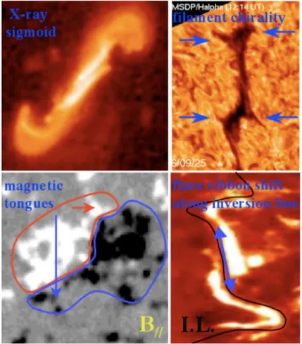
Solar magnetic fields in the North Solar Hemisphere have negative helicity, in contrast to the fields in the South Hemisphere that are governed by a positive helicity. Around 70-80% of the solar features follows this rule (see for example Pevtsov & Balasubramaniam (2003)). In Figure 1.5 we show some characteristic patterns observed in the solar atmosphere that show positive magnetic helicity, as presented by D´emoulin (2008).
When the magnetic field is closed in the integration volume (i.e it does not cross the boundary), the magnetic helicity is a gauge-invariant quantity (Berger (1999)), even though the magnetic helicity density A · B is a gauge-dependent quantity. However, when we want to study the magnetic helicity in the solar corona, we have to deal with a magnetic field that penetrates the boundaries, since magnetic flux emerges from below through the photosphere. That is the reason why Berger & Field (1984) developed the concept of relative magnetic helicity :
Hrel=
Z
(A + Ap) · (B − Bp)dV, (1.4)
where B is the magnetic field, A is the magnetic vector potential, Bp is the potential
magnetic field that has the same distribution as B at the boundary, and finally, Ap is its
corresponding vector potential, uniquely specified by the observed flux distribution on the surface with the equations
∇ × Ap· ˆn = Bn, ∇ · Ap= 0, Ap· ˆn = 0. (1.5)
In Chapter 2 we calculate the helicity accumulation in a sample of active regions using the above described relative magnetic helicity.
Figure 1.5: Some characteristic features in the solar atmosphere characterized by positive helicity: X-ray sigmoids, fibrils, magnetic tongues and flare ribbons (D´emoulin 2008)
1.4
Thesis Outline
In this thesis we investigate the trend of magnetic helicity both theoretically and observa-tionally and in different layers of the Sun. Some dynamic eruptive events observed in the corona, i.e coronal mass ejections (and more specifically halo CMEs), flares and filament eruptions for a period of two years (February 2000- June 2003) are investigated in Chap-ter 2. We use EIT/SOHO images in order to identify active regions that are possible initiation sites of CMEs. Then we use MDI/SOHO line-of-sight magnetograms that can provide us information on the photospheric magnetic field and on the velocity components of the footpoints. We then calculate the magnetic helicity injection in 10 active regions of
our sample.
The aim of the study based on observational data is to investigate the behavior of mag-netic helicity accumulation in sites where the initiation of CMEs occurred, to determine whether and how changes in magnetic helicity accumulation are temporally correlated with CME occurrence. The results obtained from the sample of events analyzed indicate that major changes in magnetic helicity flux are observed in active regions characterized by emergence of new magnetic flux and/or generating halo CMEs associated with X-class flares or filament eruptions. In some of the analyzed cases the changes in magnetic helic-ity flux follow the CME events and can be attributed to a process of restoring a torque balance between the subphotospheric and the coronal domain of the flux tubes
In Chapter 3 we investigate the magnetic helicity injection inside a supergranular convective cell by means of simulations. Taking into account the importance of super-granular cells in convection theories, we study the motion of magnetic features into such a geometrical element simplified as hexagonal cell and we analyse the results in terms of the accumulated magnetic helicity. We compute the emergence of a bipole inside the hexagonal cell and its motion from the centre of the cell towards its sides and its vertices, where the magnetic elements are considered to be sinking down. Multiple bipoles are also considered and phenomena such as cancellation, coalescence and fragmentation are also investigated. We find that the most important process for the accumulation of magnetic helicity is the shear motion between the polarities. Moreover, when magnetic bipoles move in neighboring boundaries, there is more interaction between their magnetic fields and thus a resultant higher complexity in the magnetic field configuration that leads to large amount of magnetic helicity. The closer two or more polarities are to each other, and the soonest in terms of computational run (i.e at the beginning and not at the end of the computation), the higher is their influence on the initial trend of magnetic helicity flux.
More research has to take place in both areas as described in Chapter 4. A combi-nation of observational data for longer periods with a higher angular resolution, together with a theoretical study that includes more than one hexagonal cell, able to describe the magnetic carpet configuration, can offer another piece of information in the puzzle of
the triggering mechanisms of CMEs and in their relation to other eruptive phenomena, providing more accurate predictive models.
Observational Study on Active
Regions that generate Halo CMEs
“When you set out on your journey to Ithaca, pray that the road is long, that the summer mornings are many, when, with such pleasure, with such joy you will enter ports seen for the first time; stop at Phoenician markets, and purchase fine merchandise,.. visit many Egyptian cities, to learn as much from scholars.” Konstantinos P. Kavafis, “Ithaca” (1911)
In this chapter we describe a study on the evolution of magnetic helicity in active regions (ARs) generating halo Coronal Mass Ejections (CMEs). This study can be con-sidered an attempt to give a contribution to find solutions to some hotly debated questions related with CMEs, such as to identify which, when, how and why a magnetized region can provide the necessary triggering mechanisms for the occurrence of a CME, and the con-nection, if any, with the eruption of flares. A further motivation to carry on this research
is that eruptive events such as CMEs and flares have been proposed to be primary can-didates for explaining the fact that there is not endless accumulation of magnetic helicity on the Sun (see for example Heyvaerts & Priest (1984)).
We used two types of data :
1. EIT images. Initially, we selected a sample of ARs that could be the most probable initiation sites, by working with EIT/SOHO images and by making the difference between successive images, with the pivot image being the closer to the time occur-rence of the CME. A diffeoccur-rence in brightness above a certain threshold together with the indication of a flare event were the fundamental information that allowed us to select the ARs.
2. MDI images. The parameters used in the calculation of magnetic helicity are the magnetic field, the velocity and the vector potential (see also Chapter 1). This in-formation can be obtained using the MDI/SOHO data that provide the line-of-sight component of the magnetic field. The horizontal displacement of magnetic structures can be estimated by applying a Local Correlation Technique (LCT), (November & Simon 1988).
The results obtained demonstrate that there is not a unique behaviour which can characterize the magnetic helicity injection in the ARs generating the halo CMEs and that we can distinguish between two cases. In the first case, the magnetic helicity flux shows an abrupt change before the CME occurrence pointing out the important role played by magnetic flux emergence. The second case is dealing with major changes in the helicity injection rate after the CME and the relevant physical mechanism can be rooted in the absence of a torque balance between the subphotospheric and the coronal magnetic domain.
2.1
Motivation
Two of the most controversial topics that are frequently discussed in the solar physicists community are related with the violent manifestations of the solar activity that can be
responsible for Space Weather disturbances and, when directed towards the Earth, also for geomagnetic storms. These are namely:
I) The origin site of CMEs.
II) The relationship between CMEs and flares.
Uncovering the origin of CMEs from observational data is not an easy task. Firstly, the CMEs, that are three-dimensional structures, when observed in white-light images by coronographs (either space-based such as the Large Angle Spectrometric COronograph on board SOHO or ground-based such as the Mark IV coronographs on the High Altitude Observatory that is located on top of Mauna Loa) above the occulting disk are two-dimensional projections on the plane of the sky. Therefore, not only the values of the speed and size that describe an observed CME are underestimated (since we are “missing´’ one direction) but also the linkage of any CME event with the underlying magnetic feature that is responsible for its generation, is not straightforward. Only recently, with the advent of STEREO, it has become possible to obtain more realistic information on the 3-D structure and the velocity values of CMEs (Srivastava (2010); Simon et al. (2001a)). However, the problem related to the source region of the CME, is still open. Additionally, even though it is accepted that the driving mechanism of a CME is connected to the coronal magnetic field configuration and not to the gas pressure or to the force of gravity, our knowledge on the magnetic configuration that can produce highly dynamic eruptions (such as CMEs and flares) is limited. Up to now, the development of diagnostic tools of the coronal magnetic field is quite restricted and the main observational technique for measuring the magnetic field in this outer part of the solar atmosphere, is related with radio data which can provide information on the magnetic field strength but not on the full magnetic vector. Various other methods have been developed, related with the Hanle effect in EUV lines and with the Zeeman effect in the HeI 10830 ˚A triplet (as discussed in Trujillo Bueno (2010)), but all of them are facing difficulties in providing a completely realistic picture of the coronal field. Otherwise, extrapolations methods of the photospheric magnetic field are used as proxies for the coronal magnetic field study.
Figure 2.1: From left to right: successive snapshots of full-disk AIA/SDO images acquired at 171 ˚A, obtained at 07:00 UT, 08:06 UT and 10:16 UT : ‘At approximately 08:55 UT on August 1, 2010, a C3.2 flare erupted from NOAA 1092. At nearly the same time, a filament eruption occurred, sending out a huge plasma cloud (i.e a CME) directed towards the Earth’.
Nevertheless, we also mention that our understanding of the early stages of the evolu-tion of a dynamic CME event has improved in the last decade due to the combinaevolu-tion of a large range of high quality data (such as those obtained by the Soft X-Ray Telescope on board Hinode, the Extreme UltraViolet Imaging Telescope on board SOHO, the Extreme Ultraviolet Imager on board the STEREO Spacecraft or the Atmospheric Imaging Assem-bly on board the recently launched SDO that has detected for example on 01/08/2010 a C3.2 flare accompanied by a large filament eruption, as shown in Figure 2.1) and the application of strong theoretical MHD codes (as discussed in Chapter 1).
This huge effort invested on the research on CMEs, has revealed an important aspect of their occurrence: sometimes their appearance is coincident with other dynamic events, i.e flares and filament eruptions. There is an extensive study on this topic by Khan & Hudson (2000) who showed that when a flare occurs, it can destabilize an adjacent transequatorial loop structure and thus lead to the launch of a CME. Temmer et al. (2008) have shown that there is a close relationship between the initial acceleration phase of two Halo CMEs and the impulsive phase of soft X-ray flares; Jing et al. (2004) through a statistical study,
found that 50 % of events of filament eruption are associated with the CME occurrence, whereas Gopalswamy et al. (2003b) obtained a 84 % connection between the observed filament eruptions and the CMEs; Qiu & Yurchyshyn (2005) found that the velocity of a flare- associated CME is proportional to the magnetic flux that is swept away from flare ribbons; Moon et al. (2003) found a strong connection between the kinetic energy of CME/flare limb events and the GOES X-ray peak fluxes; Chen et al. (2006) found that for CMEs that are connected to filament eruption, their velocity is roughly linearly correlated with the total magnetic flux in the filament channel.
Of course, the above mentioned studies represent just a small portion of the large literature that concerns the connection between these dynamic events, but yet a clear answer is not given.
We believe that in order to demonstrate the existence (or not) of a pos-sible connection between solar surface phenomena such as CMEs, flares and filament eruptions, it is crucial to recognize the sequence of processes, the actual conditions and the properties of the magnetic field that characterize their early manifestations. Only when a complete knowledge of this phase will be obtained, the strong basis of a CME and flare forecasting system will be constructed.
A useful tool in this respect is the magnetic helicity. As already mentioned in Chapter 1 and in accordance with Berger & Field (1984)), magnetic helicity is one of the few global quantities that remains conserved even in resistive MHD, on a timescale much smaller than the global diffusion timescale. Nevertheless, what is actually interesting is that this conservation law can break down under the occurrence of dynamic processes such as CMEs, flares and filament eruptions, that lead to large energy releases and so avoid an endless storage of magnetic helicity in the solar corona. More specifically, when a CME occurs, it releases the magnetic energy that is stored over a large volume and leads to the partial opening of the magnetic field lines. As a result, the helicity does not remain conserved in a volume on the active region scale. Moreover, the amount of magnetic helicity that can be expelled during a CME can be estimated by the variation of coronal helicity in the active
region that generates the CME (Low (1996); Green et al. (2002); Zhang et al. (2006); van Driel-Gesztelyi et al. (2002a)).
In the recent simulations of Yeates & Mackay (2009), the authors carried out global simulations of the solar corona based on photospheric observations for a period of six months in 1999. The model included the effects of flux emergence, shearing by surface motions and cancellation along with the formation and ejection of flux ropes due to loss of equilibrium. By varying the rate at which magnetic helicity was injected, the model produced 50 % of the observed CME rate over the simulated period (see also Mackay & van Ballegooijen (2006)). In contrast to this model, Cook et al. (2009) studied the number and locations of coronal null points, a key element in the magnetic breakout model, over two solar cycles. They found that the number of nulls followed a cycle variation, peaking at maximum of 15 - 17 per rotation. The vast majority of null points were located above active latitudes and lay at low heights in the corona.
Similar studies have been carried out in order to investigate how the occurrence and intensity of a flare eruption in an active region can affect the build up of magnetic he-licity in this region and the circumstances under which a CME event will be provoked. For instance, Moon et al. (2002) examined the impulsive variations that characterize the magnetic helicity when major flares associated with halo CMEs, occur. Nindos & Andrews (2004) performed a statistical study of 133 big flares of M and X class and found that in the pre-flare phase the coronal magnetic helicity of active regions producing big flares not correlated with CMEs is smaller than the coronal magnetic helicity of active regions pro-ducing CME-associated big flares. Furthermore, LaBonte et al. (2007) perfomed a survey of 393 active regions (48 X-flare producing and 345 non-X-flaring regions) and concluded that when the peak helicity flux in an active region has magnitude > 6 × 1036 Mx2sec−1
an X-class flare can take place and it will be accompanied in a few hours to few days by a CME. Work done by Hartkorn & Wang (2004) has revealed that the rapid fluctuations observed in the helicity change rate during a flare eruption, can be artifacts due to the influence of the flare emission on the spectral line during the analysis of MDI data. Thus, it is essential to focus on the long-term (i.e some days) variation of magnetic helicity in an
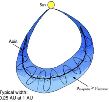
Figure 2.2: Schematic diagram of a magnetic cloud presented in Webb et al. (2000). The cloud field configuration is that of a flux rope with helical field lines. Since magnetic helicity is a conserved quantity, we can calculate and compare its value in a magnetic cloud with the amount of helicity of an active region in the corona where a CME event occurred.
active region in order to obtain accurate conclusions related to its connection to dynamic events, such as flares.
In many cases, a twisted flux tube ejected in a CME appears in the interplanetary space at a distance of 1 AU as a magnetic cloud (MC) in which the twisted nature remains well observable (Chen (1989); Forbes & Priest (1995); Qiu et al. 2007, Longcope et al. (2007)) and thus is expected to be characterized by a large amount of magnetic helicity. In this case the quantity of magnetic helicity and its conservation property can be used in order to connect a coronal surface event with its interplanetary counterpart: the magnetic helicity of a CME is expected to be very close to the amount obtained for the associated magnetic cloud (Mandrini et al. (2005); Luoni et al. (2005); Dasso et al. (2006)). In Figure 2.2 we present a schematic diagram of a magnetic cloud as given by Webb et al. (2000) were the helical field lines of the flux rope can be seen.
On the basis of these results it is clear that the study of the magnetic he-licity evolution in active regions can provide a useful tool to gain important information about the mechanisms able to produce instabilities in the mag-netic configuration. Moreover, the investigation of the magmag-netic helicity trend, before and after a CME occurrence, might contribute to our understanding of the role effectively played by these events in any eventual change in the magnetic helicity accumulation process (see, e.g., Nindos et al. 2003).
In this regard it is important to make a distinction between two cases. The former is related with the change in magnetic helicity prior to the CME occurrence, which should be further related with phenomena able to destabilize the coronal configuration, like new flux emergence or shearing/twisting of the magnetic field lines. The latter is related with changes in magnetic helicity occurring after the CME that, as suggested by Longcope & Welsch (2000) and Chae et al. (2003), might be due to the unbalance of torque between the sub-photospheric part of the flux rope and the coronal field which just lost some stress via the CME launch.
In this chapter we determine the evolution of both magnetic flux and magnetic helicity flux in active regions where a flare or a filament eruption occurred close in time with a halo CME in order to investigate the above mentioned scenarios. The choice to select halo CMEs is related to the fact that these events are generally initiated in areas located in the central part of the solar disk and this aspect is quite important when an analysis of sight magnetograms (that can provide the line-of-sight component of the photospheric magnetic field) is carried out, because in this situation possible problems related to projection effects can be avoided. We describe in Section 2.2 the selection of our sample of halo CME events and the analysis of EIT images. We first select an active region for each halo CME event accompanied by a flare or filament eruption. At a second step, we analyze the MDI magnetograms of these active regions as described in Section 1.4. The resultant magnetic helicity flux for the selected sample of active regions is given in the Section 2.4. Section 2.5 is a discussion of the significance of the results obtained. Finally, suggestions for future work are given in
Section 2.6.
2.2
Data selection and analysis of EIT images for the
iden-tification of the initiation sites of CMEs
Our aim is to study the trend of the photospheric magnetic helicity flux in active regions that generate halo CMEs.
To do this, we first selected a sample of halo CMEs from the SOHO/LASCO on-line catalog (http://cdaw.gsfc.nasa.gov/CME list/). We decided to work with events occurred close to the maximum of the 23rd Solar Cycle (when the possibility of an eruptive event occurrence is high) and we selected a total of 38 halo CME events in the time interval 2000 February 1st - 2003 June 30. We successively compared the time inferred by a back-extrapolation in time of the CME height-time trajectory with the time of a flare or filament eruption recorded in a time interval between one hour before and one hour after the CME, using the NOAA flare catalog (http://www.solarmonitor.org/index.php), in an attempt to obtain a first association between each CME and the corresponding flare or filament eruption. We choosed this time interval because it takes approximately 2 hr for a CME to cover the distance of 2R⊙ needed to reach the LASCO C2 FOV, when traveling with
a speed of 200 km/sec. This means that the reported time of the CME in the LASCO catalogue can be associated with a flare or prominence that has been detected about two hours earlier.
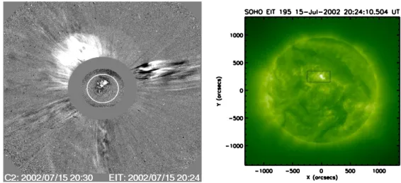
We used images acquired by the Extra-Ultraviolet Imaging Telescope (EIT) on board the Solar and Heliospheric Observatory (SOHO) as the primary data set to detect the active regions that were most probable connected to the occurrence of the dynamic erup-tions. In Figure 2.3a we show an example of a halo CME and the associated flare observed by SOHO/EIT in Figure 2.3b. The EIT instrument (see Delaboudini`ere et al. 1995 for a detailed description of the instrument), a normal-incidence telescope with multilayer-coated mirrors shown in Figure 2.4, is able to image the solar transition region and the inner corona in four narrow extreme ultraviolet (EUV) channels,as shown in Figure 2.5,
Figure 2.3: (a) Difference image showing the halo CME observed by LASCO-C2 on 2002 july 15 at 20:30:05 UT, superposed on the EIT difference image relevant to 20:24 UT ; (b) SOHO/EIT full disk image acquired on 2002 july 15 at 20:24:10 UT, showing the location on the disk of the CME source region.
Figure 2.4: The EIT instrument, described in detail by Delaboudini`ere et al. 1995
centered at:
∗ 171 ˚A, that observe the spectral lines formed by Fe IX/X and correspond to a temperature of 1.3 × 10⁶ K
Figure 2.5: From left to right: images of the solar disk acquired on 21/11/2010 by EIT: in the Fe IX/X line at 171 ˚A, in the Fe XII line at 195 ˚A (first row), in the Fe XV line at 284 ˚A and in the He II line at 304 ˚A (second row).
∗ 195 ˚A, that observe the spectral lines formed by Fe XII and correspond to 1.5 × 106 K
∗ 284 ˚A, that observe the spectral lines formed by Fe XV and correspond to 2.0 × 106 K
∗ 304 ˚A, that observe the spectral lines formed by He II and correspond to 6.0−8.0×10⁴
K
For each event we used the EIT full-disk images in the first three wavelengths. The field of view of the EIT instrument is 1024 × 1024 pixel2 with a resolution of 2.6 arcsec/pixel. The procedure used to recognize the active region responsible for the halo CME initiation
images is summarized as follows:
1. Selection of EIT full-disk images corresponding to the three wavelengths: 171 ˚A, 284 ˚
A and 304 ˚A relevant to the days of occurrence of the selected CMEs. These images are provided with 6 hr time cadence, at 01:00 UT, 07:00 UT, 13:00 UT and 19:00 UT.
2. Correction of the data for the flat field, dark current and cosmic rays. This is per-formed by using the standard EIT calibration procedure EIT PREP in Solar Software (SSW):
SSWIDL> eit prep, index,data =data, outindex, outdata, /cosmic
3. Alignment of the images using the standard SSW function drot map that rotates a map (obtained from EIT data) using the solar differential rotation formula of Howard et al. (1990).
4. Selection of a pivot image. This selection corresponds to the image obtained around the time of the CME occurrence.
5. Performing difference of images between the pivot image and the images obtained 6, 12, 18 and 24 hours, respectively before and after this image. We noted that the subtraction of images at 304 ˚A was not really useful since we could not detect significant differences between two successive images. Therefore, we decided not to work further with this wavelength. In Figure 2.6 we show running difference images in different wavelengths for two different events of our sample.
6. Selection of a box around each active region for every difference image. In Figure 2.7 we show all the selected active regions for a 24 hr difference image at 171 ˚A, associ-ated with the occurrence of a halo CME event occurred on 09/11/2002 at 13:31 UT. When the boundaries of neighboring active regions are not well-defined, the box will include both regions, so that we avoid to neglect potentially significant magnetic flux that will be later used in our calculations.
Figure 2.6: First row : Difference of EIT images acquired at 171 ˚A, relevant to the event associated to the halo CME that occurred on 15/07/2002 and was detected by LASCO/C2 at 20:30:05. The pivot image was taken at 19:05 UT. Here three images taken 18, 12 and 6 hrs earlier are subtracted from the pivot image. Second row: Difference of EIT images acquired at 284 ˚A. The halo CME occurred on 16/08/2002 and was first detected by LASCO/C2 at 12:30 UT. The pivot image was acquired at 13:05 UT and we present difference of images taken 6, 12 and 18 hrs later.
7. Obtain a set of images relevant to a single or two adjacent active regions for the period between one day before and one day after the halo CME occurrence. In Figure 2.8 we show for example the 171 ˚A difference images for NOAA 10030. The CME event occurred on 16/07/2002 and was detected by LASCO/C2 at 16:02 UT. The pivot image was acquired at 19:05 UT. From this image we subtracted the images at 01:05 UT (first panel), at 07:05 UT(second panel) and at 13:05 UT(last panel) taken on the following day.
Figure 2.7: Full-disk 171 ˚A difference image produced by the difference of the pivot image (acquired at 13:05 UT of 09/11/2002) and the image acquired 24 hrs later (13:05 UT of 10/11/2002). A halo CME occurred on 09/11/1982 and was detected by LASCO/C2 at 13:31UT. All the observed active regions are selected for further investigation.
Figure 2.8: 171 ˚A difference images for NOAA 10030. In this case, the CME event occurred on 16/07/2002 and was detected by LASCO/C2 at 16:02 UT. The pivot image was acquired at 19:05 UT. From this image we subtracted the images at 01:05 UT (first panel), at 07:05 UT (second panel) and at 13:05 UT (last panel) taken on the following day (17/07/2002).
At this stage we were able to :
(a) Select the biggest brightest and darkest area in each active region with the help of a cursor
(b) Compute the area of the bright biggest region and the area of the dark biggest region
(c) Compute the maximum intensity of the brightest area and the minimum intensity of the darkest area
8. Identify the active region that shows the largest variations in intensity and size (of brightest and darkest area) when the halo CME happens, indicating the occurrence of a dynamic event. In contrast, the other active regions show an almost constant profile in intensity.
9. Follow the same procedure with the full-disk images acquired by EIT at 195 ˚A. These data have a higher time cadence (12 minutes) than the other data (171 ˚A, 284 ˚A, 304 ˚A). In Figure 2.9 we present the graphs showing the evolution in time of the size (first row) and the intensity (second row) of the largest bright and dark areas of each active region present on the solar disk on 16/07/2002. The 0 in the horizontal axis corresponds to the image taken closer to the CME occurrence (detected at 16:02:58 UT from LASCO/C2), i.e 16:12:10 UT; from this we subtracted images with difference of 12 min until 09:36:10 UT in the same day and 00:36:10UT of the following day (no data were available from 12:36:10 UT till 13:25:59 UT). We can see in each plot that NOAA 10030 (indicated by crosses) shows a different trend than any other active region. Therefore, we considered NOAA 10030 as the initiation site of the CME.
As far as the images acquired by EIT at 195 ˚A are concerned, we stress that these data are characterized by a higher time resolution (12 minutes) than the other data (171 ˚A, 284 ˚A, 304 ˚A), characterized by 6 hr time cadence, that are nevertheless useful to study how an active region change in such time interval due to a dynamic event.
Figure 2.9: Plots of the size(first row) and the intensity (second row) of the largest bright and dark area vs. time as obtained from the difference of 195 ˚A images for each active region selected on 16/07/2002. The time cadence is 12 min. We note that the NOAA 10030 (shown by crosses) shows different trend than the other regions and thus can be considered as the most probable initiation site for the CME that was detected at 16:02:58 UT. Time 0 corresponds to the image acquired closer in time to the CME occurrence.
Thus, with images acquired at the three last wavelengths we can obtain a first idea about the candidates (i.e active regions) that are most probably connected to an eruptive event. Then, with the 195 ˚A images we can observe the evolution of these regions in short temporal periods. When a different trend (relatively to any other active region on the solar
disk) and abrupt changes are detected close to the eruption occurrence (i.e some couple of hours before and after the event), we can verify our ‘suspicious’ about the origin site of a halo CME.
Moreover, the data acquired at 195 ˚A can be quite useful in identifying dimming regions that most of the time provide information about the CME source region. Coronal dimmings are usually regarded as the consequence of removal of coronal mass during a CME eruption (Sterling & Hudson (1997); Zarro et al. (1999);Reinard & Biesecker (2008)) and sometimes appear near a flare or near an arcade brightening associated with a filament eruption (Hudson et al. (1996);Canfield et al. (1999)). Dimmings are dynamic phenomena that can develop on a typical timescale of a hour and so their evolution is fast enough and only snapshots of an active region in short time intervals can make apparent their occurrence. There appear to be two classes of dimmings: deep core dimmings (e.g Webb et al. (2000)) and more widespread dimmings coincident with the spatial extent of CMEs detected by coronographs (as investigated by Thompson et al. (2000)). Since during our analysis we are not only interested in bright areas that can be connected to a flare, but also to dark areas that can be connected to coronal dimmings, we need low time cadence data in order to recognize them. These data can only be provided by EIT at 195 ˚A.
Summarizing, we have selected 38 halo CME events and for each event we have explored the trend in brightness variations of all the active regions detected in the full-disk EIT images acquired on the same day. The double-cross check between the eruptive event registered in the NOAA report and the brightness variation inferred by the difference maps provided us a further indication about the active region that was the site of the initiation of the halo CME. In order to minimize problems related to projection effects, we focused our attention on active regions located between ±35◦
of longitude from the central meridian. With this choice, we limited our analysis to 10 active regions and, correspondingly, to 12 CMEs, because both NOAA 10030 and 10365 were the source regions of two halo CMEs. The halo CME events selected and the relevant active regions found by this method are reported in Figure 2.10, where we distinguish two classes: the first containing active regions giving rise to gradual halo CMEs, i.e. with positive acceleration (hereinafter called Class
Figure 2.10: Data on the halo CMEs and analyzed relevant eruptive events. a: the CME time indicates the time of first appearance in LASCO/C2.b: ERU indicates the occurrence of an erupting filament.
I) and the second relevant to active regions that were sources of impulsive halo CMEs, i.e. characterized by negative acceleration (Class II). In particular, this classification is based on the velocity and acceleration values of a CME:
I) gradual CMEs, characterized by velocities v ∼ 400 - 600 km s−1 and gradual
ac-celeration ( a ∼ 3 - 40 m s−2 within a distance from the Sun less than ∼ 30 R
⊙),
generally associated with eruptive quiescent filaments;
II) impulsive CMEs with higher initial velocities, in the range ∼ 750 - 1000 km s−1,
decelerating at distances ∼ 2 R⊙and generally associated with flares and eruptive
active region filaments.
This categorization has its roots on the work of Gosling et al. (1976) and MacQueen & Fisher (1983) who suggested different mechanisms for the acceleration of CMEs. More specifically, their study has revealed that the reason for the different dynamical behav-ior might be due to a different driver mechanism (or at least one with a different strength): gradual CMEs, which are events associated to eruptive quiescent prominences, are supposed to undergo a significant net propelling force over extended periods, while impulsive CMEs, which are flare-associated events, are supposed to arise from an impul-sive input into the low corona associated to flare and active region filament eruptions. This traditional classification was afterwards widely used in the study and comprehension of the kinematics of CMEs (as we can see for instance by Chen & Krall (2003); Moon
et al. (2004), Chen et al. (2006), Michalek (2009)).However, it is important to mention that this classification of CMEs has been questioned due to the fact that the study of the kinematical curve is very subjective and it depends on the performance of the in-struments, the measurement technique and the morphology of a CME. For this reason, Vrˇsnak et al. (2004) proposed the existence of a continuum of events rather than two distinct categories of CMEs since they found in both types several fast and slow events that either decelerate or accelerate. Moreover, Yurchyshyn et al. (2005) confirmed the lack of observational that can support the two-types classification of CMEs. For simplicity, we adopt this classification when analyzing our results.
2.3
Analysis and Selection of MDI images
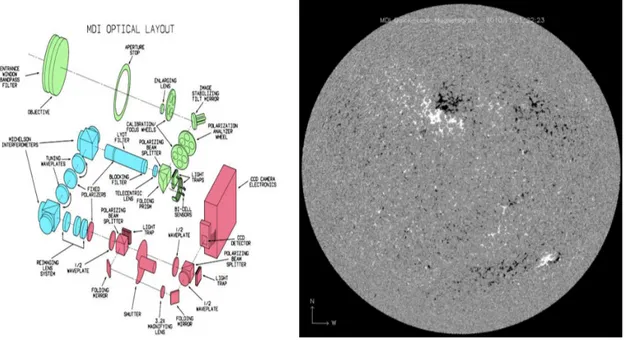
In this section we investigate the magnetic helicity flux (or rate) injected through the photosphere by using images acquired by the Michelson Doppler Imager (MDI) on board SOHO. Figure 2.11(a) shows the optical layout of MDI and Figure 2.11(b) shows a mag-netogram available at the MDI database (http://soi.stanford.edu/data/).
The Michelson Doppler Imager (MDI) instrument (see Scherrer et al. (1995) for a full description of the instrument capabilities), is designed to probe the interior of the Sun by measuring the photospheric manifestations of solar oscillations. MDI measures the line-of-sight motion (Dopplergrams), magnetic fields (magnetograms) and brightness images in full disk at a resolution of 2 arcsecond/pixel, and a fixed selected area at the disk centre in higher resolution (0.62 arcsecond/pixel). As far as magnetograms are concerned, they show the distribution of the magnetic field across the solar disk, obtained by measures of the magnetic strength using Zeeman splitting of the N iI photospheric line at 6767.8 ˚A.
In Figure 2.12(a) we present an EIT/SOHO image of the active region NOAA 10030 which was identified by the previously mentioned double check as the source region of the halo CME that occurred on 15/07/2002 at 20:30:05 and in Figure 2.12(b) we show the MDI/SOHO magnetogram relevant to NOAA 10030, acquired at 20:30 UT.