Four essays on regional growth and other related issues: evidence from the Russian Federation and the Indian Union

UNIVERSITÀ DEGLI STUDI DI ROMA

"TOR VERGATA"

FACOLTA' DI ECONOMIA

DOTTORATO DI RICERCA IN ECONOMIA INTERNAZIONALE

CICLO DEL CORSO DI DOTTORATO

FOUR ESSAYS ON REGIONAL GROWTH

AND OTHER RELATED ISSUES

(Evidence from the Russian Federation and the Indian Union)

Tullio Buccellato

A.A. 2008/2009

Docente Guida/Tutor: Prof. Pasquale Scaramozzino

Coordinatore: Prof. Giancarlo Marini

ii First of all I should say thanks to my PhD supervisor Prof. Pasquale Scaramozzino, who has been constantly following the state of my works. Very helpful were also all the hints received by Prof. Laixiang Sun, Prof. Wendy Carlin and Fabrizio Adriani. A special thanks go to the people who have directly contributed to the realization of some of the chapters collected in the thesis: Tomasz Marek Mickievicz, Michele Alessandrini and Francesco Sant’Angelo.

This thesis consists of four separate chapters, which are all in themselves self standing. The first three papers refer to the Russian Federation context, while the last one to the Indian Union’s one. The liaison linking all the works is represented by the use of econometrics techniques, which better adapt to regional datasets and, in the most of cases, this implies the use of spatial econometrics tools. Here below I briefly summarize the contents and main findings of each of the chapters. The first paper analyses the process of convergence across Russian regions using spatial econometrics tools in addition to the traditional β-convergence techniques as derived from the neoclassical theoretical setting. The study covers the period 1999-2004. Absolute convergence is absent, confirming the results obtained in previous studies on the Russian Federation. The β convergence coefficient begins to be significant only after the introduction of other explanatory variables in addition to the initial level of per capita income. The neoclassical conditional convergence model is found to overestimate the absolute value of β with respect to its spatial lag model counterpart, strengthening the hypothesis of a bias due to spatial dependence in the data. When moving to the panel data analysis, the gap in convergence coefficient becomes more evident and slightly present also in the spatial error model. The spatial component appears to be non-negligible and, consequently, conventional convergence estimates suffer a bias due to spatial dependence across observations. Furthermore, variables such as hydrocarbon supply, openness to trade and FDI per capita are found to have an unambiguous, positive and statistically significant impact on growth. Results are also confirmed by the panel data specifications of the models. The second chapter focuses on the role of hydrocarbons as a possible determinant for inequality. Already in the first chapter I showed that hydrocarbons are one of the main elements constituting the great divide across fast and slow growing Russian regions. Here we concentrate mainly on the role of oil and gas as a possible determinant of within region inequality. After having reviewed the economic literature concerning determinants of inequality across countries and within Russia, we test empirically the determinants of intra-regional inequality in Russia, applying robust dynamic panel data estimators. We find that regions where oil and gas is produced tend to experience higher levels of income inequality in striking resemblance to cross-country results.

The third chapter is devoted to the analysis foreign direct investment in Russia. More in particular, we explore the hypothesis of spatial effects in the distribution of Foreign Direct Investments (FDI) across Russian regions. We make use of a model, which describes FDI inflows as resulting from an agglomeration effect (the level of FDI in a given region depends positively on the level of FDI received by the regions in its neighbourhood) and remoteness effect (the distance of each Russian iii

iv over the period 2000-2004 we find that the two effects play a significant role in determining FDI inflows towards Russia. The two effects are also robust to the inclusion of other widely used explanatory variables impacting the level of FDI towards countries or regions (e.g. surrounding market potential, infrastructures, investment climate).

The fourth and last chapter, we investigate the process of convergence/divergence across Indian states. After surveying the main economic reforms implemented during the last decades in the Indian Union, we conduct an econometric study of the determinants of economic growth in the neoclassical frame of the Solow model. One of the main novel aspects of our convergence analysis is the attention paid to the spatial pattern of growth across Indian states. Making use of spatial econometric tools, we control for two different kinds of spatial interaction: distance and neighbourhood. Our results suggest that the gap between poor and rich states has constantly increased during the 1980s and the 1990s. Specifically, we find that winners were those states that benefited the most from the recent process of reform and liberalization, thanks also to their geographical advantage and to the presence of a developed service sector. Losers were instead the landlocked and highly populated states with a predominant agricultural sector and a low level of innovation.

v

Chapter 1: Convergence across Russian Regions: A Spatial Econometrics Approach………..1

Chapter2: Oil and Gas: a Blessing for Few Hydrocarbons and Within-Region Inequality in Russia1...38

Chapter3: Foreign Direct Investments Distribution in the Russian Federation: Do Spatial Effects Matter?2...70

Chapter4: Whither the Indian Union? Regional Disparities and Economic

Reforms3_{……….…98}

1 _{This paper was written with Prof. Tomasz Marek Mickievicz.}

2 _{This paper was written with Prof. Pasquale Scaramozzino and Michele Alessandrini.} 3 _{This paper was written with Francesco Sant’Angelo.}

Chapter 1:

Convergence across Russian Regions: a Spatial Econometrics Approach

1.1. Introduction

On December 25, 1991, the Russian communist period was officially over. This was indeed the day in which the last general secretary of the communist party Mikhail Gorbachev left the Kremlin, signing the definitive end of the central planned economy and the beginning of the transition to the market economy.

The Russian transition has been one of the most arduous that the group of former central planned economies has experienced. The sharp fall in output followed by a strong increase in unemployment, together with the explosion of inflation and the increase of government debt are some of the well known challenges Russia had to face during its first years of transition. The August 1998 financial crisis, however, represented a turning point, after which the Russian Federation started again to grow at a sustained pace.

The recovery, which started in 1999, has been mostly the result of the sharp increase in international hydrocarbons prices. Massive exports of oil and gas have restarted the engine of the Russian economy ensuring a sustained annual average rate of growth over 5% during the period 1999-2004. However, within the Russian Federation rates of growth have been highly heterogeneous across regions. Income dispersion has constantly increased over the recovery period, and, as a result , together with areas experiencing remarkably improved living standards there are still regions which appear to be trapped to poverty.

The group of regions that has experienced the highest rate of growth is the one within the Ural Federal District. This is however in line with the stylized fact of the oil export-led growth characterizing the post-financial-crisis recovery. The Tyumensk region, together with the two autonomous regions of Yamalo-Nenetskiy and Khanty-Mansiyskiy belonging to it, accounts for more than half of the total hydrocarbons production of the entire Russian Federation. The rapid pace of growth of these regions is one of the main sources of divergence in level of GDP per capita. The Ural area is indeed not only the leader in the rate of growth, but also region with the highest GDP per capita during the initial period 1999.

Besides the natural resources determinant and in strong connection with it, a key component which affects regional patterns of growth in a heterogeneous fashion is represented by the geographic location. Russia encompasses the largest territorial extension worldwide. Distances play a major role in terms of trade, knowledge spillovers and factor movements. The easiest way to highlight the

importance of geographic location for the economic performance, is to divide Russian territory into three distinct parts with respect to the Tyumensk area. All regions around this area have performed better than the others relative to their initial conditions in level of GDP per capita, which was already comparatively high. The western and the eastern parts share a common characteristic- for both of these areas regions experiencing higher rates of growth are the ones in their northern parts. Accordingly, one of the areas which have been touched only marginally by the economic recovery is the Caucasus zone. This portion of territory includes the region which has registered the worst economic performance over the period considered, even if starting from the lowest initial level in GDP per capita, which is represented by the Republic of Ingushetia. This last one has probably suffered the most from the instability of the area induced by the Chechen war. Until 1994 Ingushetia and Chechnya constituted a single republic and after that year Ingushetia became formally independent, but effectively still very vulnerable to what happened beyond its border. Still belonging to this area but enjoying a much better performance, Dagestan Republic was able to switch its position in the distribution of income per capita across Russian regions reaching a higher percentile. However, it must be taken into account that Dagestan's major exports are oil and fuel. The poorest area remains however the South Siberia, where a consistent part of the population lives under the poverty line. Regions such as the Republic of Altai and the Republic of Tyva appear completely locked to poverty and their inhabitants unable even to face costs barriers for migration towards more prosperous regions or countries.

The case of the capital Moscow deserves particular attention. Moscow has indeed exhibited a very high rate of growth, representing not only the administrative capital of the federation but also the financial capital and the centre of the main economic and political interests. However, the wealth is very unevenly distributed across inhabitants. The income per head has on average reached Western European standards but this is not representative for the greatest part of the population. Moscow has indeed registered the highest level of inequality in the federation-the Gini index registered by Goskomstat (Federal State Statistics Service) for the year 2003 has been 0.615. Such a level of inequality reflects the problem of an incomplete transition, which created an oligarchic structure of the society, leaving out of the economic transformation large parts of the population (especially elder generations). Nonetheless, in the recent years a newly-born middle class is strengthening in the urban contexts of the federation and especially in its capital, giving the perception of a more equal distribution of wealth across households.

Due to natural resources and the geographically concentrated industrial structure inherited from the Soviet era, Russia’s regions have performed heterogeneously depending on their position over the huge extension of the federal territory. Thus, many studies concerning regional patterns of growth

in Russia have assigned an important weight to the geographic factor through the introduction of control variables, such as distance from the capital Moscow, dummies for the European part, landlocked regions, permanent sea access and other geographic characteristics.

The main purpose of this paper is to explicitly relax the assumption of spatial independence across the observations. The use of a regional dataset implies consideration of the possibility that observations are not independent, as a result of the inter-connections between neighbouring regions (Anselin 1988). Many convergence studies based on the neoclassical framework (Solow 1956 and Swan 1956) rely on the assumption of closed economies. If this assumption can appropriately be applied to the datasets of countries, it instead appears more restrictive and strong for regions within a single country. Therefore, many regional studies can suffer from serious bias and inefficiency when it comes to making convergence coefficient estimates and to accounting for possible variables affecting growth rates.

In order to deal with this problem, the present paper examines the elements that enhance divergence in levels of per capita income across 77 regions of the Russian Federation. It applies cross-sectional and panel spatial econometric methods (lag and error models) to assess the impact of hydrocarbon supply and other variables relevant to regional economic growth. As will be examined in detail, oil and gas production constitute the main driving force behind divergence across regional growth patterns. The results obtained from both the cross section and the panel analysis confirm the importance of taking into account spatial interactions across regions. In particular, as one includes the spatial lag of the dependent variable in the model, the convergence coefficient assumes a lower magnitude. This seems to confirm the hypothesis that the spatial dimension cleans up the convergence coefficient from the already mentioned effects of trade, knowledge spillovers and factor movements, which become stronger among contiguous regions. Section 2 begins to introduce the spatial econometric models to be used in addition to the traditional neoclassical convergence analysis tools; section 3 is devoted to the description of the dataset used for the empirical part of the study; section 4 illustrates results obtained by implementing an absolute convergence study and compares the results with its spatial counterparts. After providing evidence of divergence in levels of GDP per capita, Section 5 proceeds toward a conditional convergence approach, which, once again, is compared to the results obtained using spatial econometrics tools. Section 6 extends results to the panel analysis. Conclusions follow.

1.2. The Model

The spatial econometrics approach is increasingly being used in the study of convergence. The neoclassical approach to β-convergence (Barro and Sala-i-Martin 1991,1997, 2003) relies on the decreasing marginal productivity of capital assumption, implying that richer countries endowed with more capital tend to grow more slowly than poorer ones (absolute convergence). However, the pace of growth depends also on the distance from the country-specific steady state, i.e. the further a country finds itself from its own steady state, the faster its growth rate will be. Assuming a kind of reversed gravity law, specific factors must be considered that could potentially affect the convergence process (conditional convergence). Accordingly, the following two models have been implemented for convergence studies:

i i i T i _y y y T _=α+β +ε      ×ln ln( ) 1 0 , 0 , , ₍₁₎ i i i i T i _{y X} y y ε γ β α+ + + =         × ' 0 , 0 , , _{ln( )} ln T 1 t i, (2) ε ~ i.i.d(0,σ2In) y

where is the GDP per capita of country or region i as of date t, T is the length of the period, is a constant and β is the convergence coefficient. Specification 2 also includes the matrix X containing additional explanatory steady-state variables (physical or human capital, shares of production sectors to GDP, degree of political instability, ratio of public expenditures to GDP and other environmental variables) and the respective vector of associated coefficients γ. As coefficient β is negative and statistically significant, the cross section of countries or regions exhibits β-convergence.

α

However, both specifications 1 and 2 rely implicitly on the assumption that the observations are geographically independent. If this assumption can adapt well to cross-sections of countries, it becomes very strong for regional studies, for which it appears more plausible to assume spatial interactions among observations. In cases where spatial correlation is detected, OLS estimates turn out to be biased and thus more suitable spatial econometrics tools are required (Rey and Montoury 2000; Le Gallo, Ertur and Baoumont 2003; G. Arbia, R. Basile and G. Piras 2005).

Since the main purpose of this paper is to examine not only the convergence process in levels of GDP per capita but also to assess the impact of some environmental variables on economic growth, we will use the spatial counterparts of both absolute and conditional convergence models. For each specification we compare estimates obtained using spatial lag and spatial error models, which yielded four different benchmark models:

i T i i T i y y T W y y y T α β ρ _+ε           × + + =       × , 0 , , _{ln( )} 1 _ln ln 1 i i      ,0 ,0 (1a) (2a)

(

)

(

)

where specifications 1a and 2a represent the so called spatial lag model and 1b and 2b the spatial error model. W is a binary contiguity matrix expressing neighbouring regions by 0-1 values. The value 1 is assigned in the case that two regions have a common border of non-zero length, i.e. they

are considered first order contiguous; ρ and λ represent spatial autoregressive coefficients for the dependent variable and the error respectively, and ε is a vector of error terms considered independently and identically distributed.

Spatial lag and spatial error model represent two different approaches to address the issue of spatial heterogeneity. In the first specification, the parameter ρ could be interpreted as a measure of spatial interaction across contiguous regions. In other words, the spatial lag model consents to quantify how the rate of growth in a region is affected by the one in its surrounding regions. However, the spatial lag is a stochastic regressor always correlated with ε through the spatial multiplier4, which makes OLS estimates biased and imposes the use of more suitable Maximum Likelihood estimators. On the other hand, the coefficient λ present in the spatial error model measures the degree of spatial autocorrelation between error terms of neighbouring regions. In this case, since the errors are non-spherical, OLS would provide inefficient estimators and Maximum Likelihood estimator is again preferable.

One possible drawback of the cross-sectional estimates could be represented by omitted variables and heterogeneity generated bias. The use of panel data allows to overcome this problem through the control of regional specific effect. It is then not surprising that growth studies have made an increasing use of fixed effect estimates to complete cross-sectional studies and to check for their robustness. The panel specification for the absolute convergence model takes the following form:

t i t i i t i k T i _y y y , , , , _{ln( )} ln _=α +β +ε       ₊ (3)       + t i k T i y_, , ln

where is the annual growth rate of income per head and ln( is the log of per capita income at the beginning of each period. Peculiar to this model is the presence of the time invariant regional specific effect represented by the parameters α . This set of parameters can be either assumed as fixed or random, generating the fixed effect and the random effect panel data models respectively. To our purposes, given that our observations are not randomly drawn but represent 77 regions composing the Russian federation, the use of the fixed-effect specification appear more suitable.   y ) ,t i y i

4 _{Notice that equation 1a can be rewritten as}

[

]

i i i T i _{I W y} y y T __× −ρ =α+β +ε              ×ln ln( ) 1 0 , 0 , , .

Starting from the traditional fixed-effect specification we can account for spatial dependence either introducing a time varying spatially lagged term of the dependent variable (fixed-effect spatial lag model), or leaving unchanged the systematic part of the model introducing the spatial component in the error term (fixed-effect spatial error model). Proceeding this way we obtain the two spatial counterparts of Equation 3: t i T i t i i k T i y y T W y y y T , , , , _{ln( )} 1 _ln ln 1 _{α β ρ +ε}           × + + =       × + t i t i,    ,   (3a) t i t i i t i k T i u y y y , , , , ) ln( ln _= + +       × + _{α β} T 1 t i t i t i, =λWu, +ε, (3b) u

because the time invariant variables included in the cross-sectional conditional convergence analysis can not be included in the traditional fixed-effect panel data model, we will limit the panel data analysis just to the absolute convergence specification. However, being the spatial fixed effect counterpart a non-linear estimator which allows to account also for possible time invariant variables, we will display such results together with the traditional random-effect results in section 6b.

1.3. Data Description

The Russian Federation is characterized by a very complex administrative organization. The first major administrative division includes seven federal districts (Central Federal District, North West Federal District, South Federal District, Volga Federal District, Ural Federal District, Siberian Federal District, Far Eastern Federal District). Each federal district is sub-divided into a series of entities that can take one of three different forms: oblast (region, province), kraj (territory) and republic. Some regions are further sub-divided into entities classified as autonomous regions (Avtonomnje Okrugi).

The only reliable dataset for the Russian Federation is the one collected by Goskomstat providing data for 89 regions. This source however suffers from several limitations. Data are either completely missing or sporadically available for ten of the regions, which are, therefore, to be excluded from this analysis. Indeed, data on the Chechen Republic are entirely missing for all the

variables included in the analysis5_{. Data are also incomplete for nine autonomous regions-Nenetsia,}

Parma, Yamalo-Nenetskiy, Khanty-Mansiyskiy, Taymyr, Evenkia, Ust-Ord Buriatia, Aghin Buriatia and Koryakia-yet it must be pointed out that the majority of these are treated as parts of other Russian regions and, as a result, are included in the study, albeit at a more general level of aggregation.

The only autonomous okrug with a fully available dataset is the Chukotka region, which, nevertheless, represents an outlier for the majority of estimates performed and thus was eliminated as well. The last variable excluded from the analysis was the region of Kaliningrad, for reasons deriving directly from the spatial econometrics tools implemented, which require observations to have at least one border in common with another region. The Kaliningrad region is an enclave, which, by definition, is surrounded by other countries, representing an outpost of Russian territorial jurisdiction. In total, we end up with a dataset of 77 regions that also includes the cities of St. Petersburg and Moscow.

Remaining to be defined is the period over which the analysis can be implemented. In the case of Russia we would be tempted to use all the available data from the beginning of the transition period, but the GDP had slumped dramatically in the period leading up to the 1998 financial crisis, which was a turning point, and recovery only began in 1999. The non-monotonic growth path makes in principle critical the use of the complete series, reducing the available period after the structural break following the financial crisis of 1998.

As suggested by L. Solanko (2003), it would be more appropriate to break the series into two parts and implement separate convergence analyses for the two sub-periods. Nonetheless, data are not available for many variables over the period 1992 to1998 and the use of initial values in order to avoid possible problems of endogeneity among variables is crucial to the conditional convergence analysis.

It must also be remarked that the first period of transition is characterized by strong instability in all the principal economic indicators and, for this reason, it is difficult to be assumed as the basis for any kind of economic analysis. For all these reasons, the analysis covers the years from 1999 to 2004.

1.4. Absolute convergence analysis

1.4.1. Neoclassical Estimates of Absolute β-Convergence

Our empirical analysis starts with a neoclassical regression of absolute convergence across 77 Russian regions in the period 1999-2004. Hence, we consider equation 1 and we perform cross-sectional OLS estimates of unconditional β-convergence. If convergence holds, we would expect a negative and significant coefficient for the variable referring to the initial condition, considering as dependent variable the average growth rate over the period considered6.

Illustrated in Table 1 are the results of an OLS-based absolute β-convergence regression. The coefficient associated with the initial level of per capita income is negative but completely non-significant. It can thus be concluded that Russian regions experienced divergence during the recovery period that began in 1999. This is in contradiction with L. Solanko's detection (2003) of a significant annual convergence rate of approximately 3%. However, the number of observations used was 76 and the period considered was from 1992 to 2001, which confirms the difficulty of considering the entire series starting from 1992.

6 _{The complete specification of unconditional convergence model is: 1/5∗ln(y}

i,2004/yi,1999)=α+β∗ln(yi,1999))+εi where i=1,2,…,77

Table 1: Absolute β-convergence of per-capita income in 77 Russian regions (1999-2004)-OLS Estimates

(numbers in brackets refer to standard errors) .2905711** Constant (.0808582) -.0047008 ln(y1999) (.0081331) Goodness of Fit R2 _0.0044 Observations 77 Log Likelihood 145.2157 Regression Diagnostic 0.93 Breush-Pagan heteroschedasticity test (0.3352) 22.19456

White heteroschedasticity test

0.000015 3.246 Moran's I spatial autocorrelation test (0.001) 8.438 LM test (error) (0.004) 8.424 LM test (lag) (0.004) 16.00371

Jarque-Bera normality test

(0.000335) * significant at 10%; ** significant at 5%; *** significant at 1%

Table 1 also displays diagnostic statistics detecting possible misspecifications of the convergence regression. Two interesting considerations can be made: first, we cannot reject the null hypothesis

of homoskedasticity in a Breush-Pagan test on the residuals, while the White test exhibits opposite results; second, the Moran I test7 _{significantly detects spatial autocorrelation, which is also}

confirmed by the two Lagrange Multiplier tests. Particular caution must, however, be used in interpreting these results because the Jarque-Bera test indicates that residuals are non-normally distributed.

At this stage we must address the problem of heteroskedasticity, considering spatial dependence as its only possible source (Anselin and Griffith 1988). We shall then proceed with our analysis by attempting to assess which of the two forms of spatial interaction is present, given that the two Lagrange Multipliers tests presented in Table 1 do not provide a clear answer to this question.

1.4.2. Spatial Econometrics Analysis: Spatial Lag vs. Spatial Error Model

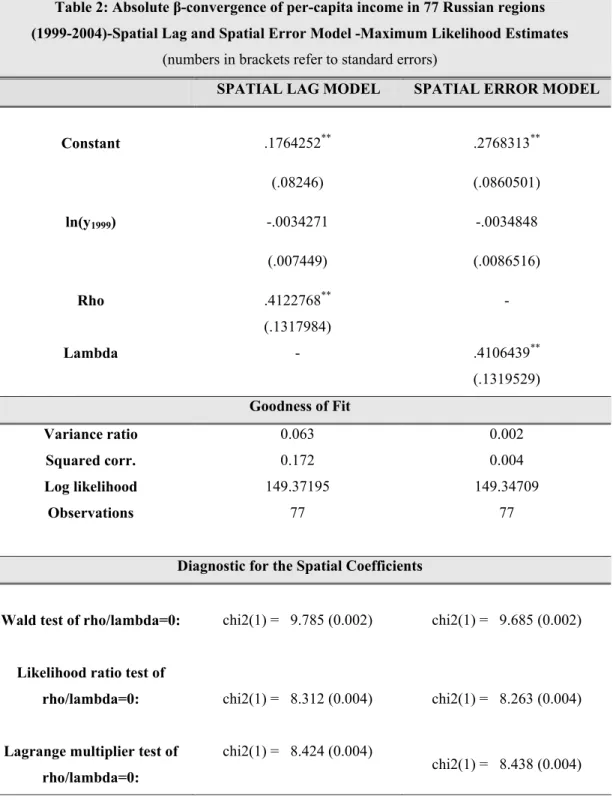
OLS results appear to suffer from a misspecification induced by omitted spatial dependence terms, as well as other possible variables conditioning patterns of convergence (to these other variables we will address our attention in the next two sections). As already discussed, the assumption of spatial independence can often prove overly restrictive for cross-sectional studies conducted at a regional level. In this section we allow for spatial interdependence across observations, estimating models 1a and 1b for the spatial lag and spatial error models, respectively. Estimates are made through a maximum likelihood estimator in order to avoid the aforementioned problems of endogeneity and inefficiency in OLS estimates8_{, which include a spatially lagged}

regressor among the explanatory variables.

Table 2 displays the results implemented by considering possible interactions between observations across space. Both the coefficients of the spatial lag term and the spatial error term appear large in magnitude and very significant. The coefficients associated with the initial per capita income level remain not significant and decreased in absolute value. Though results are weakened by the low level of significance, the decreased convergence coefficient seems to confirm the presence of the positive effect induced by factor mobility, which becomes stronger among neighbouring regions. Nonetheless, it still appears difficult to discriminate between the spatial lag and spatial error models. The only difference comes from the goodness of fit (variance ratio, squared correlation and Log likelihood, this latter component being negligible), which seems to work in favour of the spatial lag specification. To have a more accurate idea of which model fits better the dataset, it is

7

Moran's I tests the null hypothesis of no spatial autocorrelation and has an asymptotic normal distribution. 8 _{Estimates are performed using the spatial regression STATA package, elaborated by Maurizio Pisati of the} Department of Sociology and Social Research at the University of Milano Bicocca .

necessary to investigate for other possible factors that exacerbate divergence across regions in order to better disentangle the effects of regions-specific characteristics and geographic interactions - in other words, it is necessary to move towards a conditional convergence analysis.

Table 2: Absolute β-convergence of per-capita income in 77 Russian regions (1999-2004)-Spatial Lag and Spatial Error Model -Maximum Likelihood Estimates

(numbers in brackets refer to standard errors)

SPATIAL LAG MODEL SPATIAL ERROR MODEL

Constant .1764252** _.2768313** (.08246) (.0860501) ln(y1999) -.0034271 -.0034848 (.007449) (.0086516) Rho .4122768** _- (.1317984) Lambda - .4106439** (.1319529) Goodness of Fit Variance ratio 0.063 0.002 Squared corr. 0.172 0.004 Log likelihood 149.37195 149.34709 Observations 77 77

Diagnostic for the Spatial Coefficients

Wald test of rho/lambda=0: chi2(1) = 9.785 (0.002) chi2(1) = 9.685 (0.002)

Likelihood ratio test of

rho/lambda=0: chi2(1) = 8.312 (0.004) chi2(1) = 8.263 (0.004)

Lagrange multiplier test of rho/lambda=0:

chi2(1) = 8.424 (0.004)

* significant at 10%; ** significant at 5%; *** significant at 1%

1.5. Conditional Convergence Analysis 1.5.1. Possible Determinants of Divergence

Russian economic recovery in the period from 1999 to 2004 was mainly dependent on its hydrocarbon supplies. The price of crude oil and natural gas has risen sharply since 1999 and there is substantial evidence of a positive relationship between GDP growth in Russia and oil prices. Natural resources represent a prominent share of industrial production, 80% of which is accounted for by mining products, along with metals and precious stones. In 2003 oil and gas accounted for 49% of exports and constituted 17.1% of GDP (Gurvich 2004).

Growth driven by oil production is a phenomenon that not only characterizes Russian post-transitional recovery, but one which has historically been a primary source of economic prosperity for the Soviet Union since the 1917 revolution (J.I.Considine, W.A.Kerr and E.Elgar 2002). Oil production was already at a level of approximately 25 million barrels by 1920, and in the year 1987/88 it peaked at 4.5 billion barrels, making Russia the largest oil producer in the world. The early 1990s were characterized by a marked inefficiency in oil reserve management and Russia dropped back to third place among oil producers, behind Saudi Arabia and United States.

Natural resources represent a major portion of Russia's wealth and are very unevenly distributed across the Federation. As of 1999 nearly 58% of oil and gas production was concentrated in Tyumensk region, which, however, includes the two autonomous okrugs of Yamalo-Nenetskiy and Khanty-Mansiyskiy. The substantial heterogeneity in hydrocarbon supply is probably the first factor that exacerbates divergence among regions. In this context, geographic position takes on a very important strategic function: sharing borders with regions rich in natural resources can be considered a key asset in growth enhancement. It is not surprising then that the Tyumensk region had the highest GDP per capita throughout the period in question, nor that the regions surrounding it were among those enjoying the highest growth rates.

Other variables included in the growth regression of the conditional convergence analysis are the three most significant ones selected from a group of six. Accordingly, we consider the impact of variables such as international openness to trade (ratio of exports plus imports to GDP), R&D (share of the population employed in research and development) and FDI per capita. The three remaining variables, which appear only marginally related to growth, are: health services (numbers

of doctors per capita), crime (natural log of registered crimes out of 100,000 inhabitants) and fixed per capita investment9_.

Furthermore, a dummy is included for the Republic of Ingushetia. Ingushetia was the Russian region with the lowest growth rate in the period from 1999 to 2004, even though its initial conditions were very low, which is completely at odds with the neoclassical theory of convergence. This region was part of Chechnya until 1992 and is probably the one that suffered the most from the instability caused by the ongoing civil war. However, it would be improper to include Ingushetia in a war dummy, since at the moment it is separate from Chechnya. Ingushetia's economy is highly dependent on imports mainly coming out of CIS and has, by far, the highest share of imports to GDP of all the regions. The inclusion of a dummy for Ingushetia is thus important also for the sake of avoiding a series of disturbing and misleading effects on the international openness variable.

1.5.2. Neoclassical Conditional Convergence Analysis

The conditional convergence analysis is conducted using the specification 2 in section 2. This model is in line with the empirical growth literature, which regresses as dependent variable the average annual growth in per capita income on the initial level of per capita income and other explanatory variables assumed to be proxies of different steady states (Barro and Sala-i-Martin 2003).

Table 3 summarizes the results of the conditional convergence implemented by using a simple OLS regression. As we consider explanatory variables as possible growth determinants, the coefficient attributed to the initial income conditions becomes very significant, its absolute size increases denoting a conditional β-convergence rate of about 3.6%. As expected, the most significant variable in conditioning growth is the share of oil and gas extraction to GDP per capita. However, the high impact emerging from the regression is mainly due to the contribution of Tyumensk10. Openness to trade played also an important role in enhancing growth in the five years considered in the analysis. The coefficient is positive and significant as long as we include the dummy for Ingushetia Republic in the regression. The share of employees in R&D has a positive but only marginally significant coefficient while regions able to attract more foreign capital are shown to perform better on average than the others. Openness to trade also played an important role in enhancing growth in the five years considered in the analysis. The coefficient is positive and

9 _{All the figures concerning the above mentioned variables are taken from Goskomstat's Regiony Rossii 2004.} 10 _{The coefficient for the variable of oil and gas remains strong and significant also in a regression robust to the} presence of outliers.

significant as long as we include the Ingushetia Republic dummy in the regression. The share of R&D employees has a positive but only marginally significant coefficient while regions able to attract more foreign capital displayed better performance on average than the others.

The goodness of fit undergoes a substantial increase, since now 34% of the variance of growth rates is fully explained by the variables included in the survey. Nonetheless, the regression diagnostic continues to detect the presence of heteroskedasticity and spatial autocorrelation across the observations. The Jarque-Bera statistics improve, but not sufficiently enough to state that residuals are distributed normally. Hence, test results are still to be considered with caution.

The Lagrange Multiplier spatial error and spatial lag term tests show a difference that is more marked than in the absolute convergence regression. Both spatial error and spatial lag appear to be present, but the LM-test for residual spatial lag dependence is clearly more significant. This leads to a closer consideration of the possibility that our observations have violated the independence assumption and that, therefore, the OLS estimates are biased and inefficient. However, we cannot entirely exclude the possibility of correlated error terms across space, which would produce inefficiency.

Table 3: Conditional β-convergence of per-capita income in 77 Russian regions (1999-2004)-OLS Estimates

(numbers in brackets refer to standard errors)

.5871611*** Constant (.0831493) -.0365959*** ln(y1999) (.0085534) .0695902*** Oil and Gas

(.0158596) .514478** Openness to trade (.2016898) .0012978* R&D (.0007735) .0000393** FDI per capita

(.000018)

(.0563711) Goodness of Fit R2 0.3431 Observations 77 Log Likelihood 164.3892 Regression Diagnostic 1.19

Breush-Pagan heteroschedasticity test

(0.2760) 44.41333

White heteroschedasticity test

(0.002066) 2.872

Moran's I spatial autocorrelation test

(0.004) 5.525 LM test (error) (0.019) 7.400 LM test (lag) (0.007) 13.99277

Jarque-Bera normality test

(0.000315) * significant at 10%; ** significant at 5%; *** significant at 1%

1.5.3. Spatial Lag vs. Spatial Error Model for the Conditional Convergence Analysis

In this section we analyse and compare the results obtained with the spatial counterparts of the conditional convergence model. In other words we refer to specifications 2a and 2b of section 2. Consideration must be given, first of all, to which of the two model specifications seems preferable. The addition of conditioning variables to the convergence regression has substantially improved the explicative power of the set of statistics necessary to discriminate between the two models. The goodness of fit of the lag model is admittedly better than the one obtained from the error model, both in terms of variance ratio and log likelihood. All the diagnostic tests on the spatial

coefficients indicate a higher robustness and significance of the lag coefficients. Furthermore, results obtained with the error model are much more in line with the OLS regression results.

All these results confirm that, for the cross-sectional analysis, the spatial lag model is more suitable to explaining the convergence process across Russian regions over the period considered. Noteworthy is the fact that this specification displays a lower convergence rate than the neoclassical conditional convergence model. The spatially lagged dependent variable captures positive geographic spill-over effects across regions sharing the same borders, which normal growth regressions tend to attribute to the initial conditions in per capita income. In other words, the neoclassical specification of conditional convergence tends to overestimate the β coefficient. Interesting considerations can also be made for the coefficients attributed to the other explanatory variables included in the regression. The two variables relating to hydrocarbons and openness to trade remain both significant and positive in their impact on average growth. However, their contribution is somehow rescaled with the introduction of the spatial components. The share of R&D employees in the population becomes completely insignificant, though its level of significance was already low in the neoclassical specification of convergence. The ability to attract foreign investments is the only variable that undergoes an increase both in significance and in absolute value of the coefficient. The dummy for Ingushetia remains highly significant but with a lower coefficient in both the spatial specifications.

A further comment is required, i.e. that at this stage we are not considering other possible sources of heteroskedasticity related to causes different from spatial autocorrelation, since residual heteroskedasticity analysis is beyond the scope of this paper. Nevertheless, reported in the Appendix C are the results of estimates with robust standard errors for all the models treated and these results do not appear substantially different in their essence.

Table 4: Conditional β-convergence of per-capita income in 77 Russian regions (1999-2004)-Spatial Lag and Spatial Error Model -Maximum Likelihood Estimates

(numbers in brackets refer to standard errors)

SPATIAL LAG MODEL SPATIAL ERROR MODEL

Constant .4626981*** .5852261***

(.0849754) (.0870229)

ln(y1999) -.0327028*** -.036175***

(.0077305) (.0089695)

.0637439*** _.0646275***

Oil and Gas

(.0142636) (.0149055) .4491642** .4074767** Openness to trade (.1810044) (.178504) .0008427 .0009499 R&D (.0007057) (.0008011) .0000423 .0000459***

FDI per capita

(.0000161) *** (.0000156) -.2393965*** _-.225246*** D_Ingushetia (.050748) (.0503513) .3606414** - Rho (.1206447) - .3970674** Lambda (.1414236) Goodness of Fit Variance ratio 0.434 0.340 Squared corr. 0.473 0.389 Log likelihood 168.33404 167.66079 Observations 77 77

Wald test of rho/lambda=0: chi2(1) = 8.936 (0.003) chi2(1) = 7.883 (0.005) Likelihood ratio test of

rho/lambda=0: chi2(1) = 7.890 (0.005) chi2(1) = 6.543 (0.011) Lagrange multiplier test of

rho/lambda=0:

chi2(1) = 7.400 (0.007)

chi2(1) = 5.525 (0.019) * significant at 10%; ** significant at 5%; *** significant at 1%

1.6 Panel Data Convergence Analysis. 1.6.1. Traditional Panel Estimates

In this section we report results of the traditional panel analysis as specified in equation 3 of section 2. Table 5 displays results for three possible specification which are the absolute convergence with random and fixed effects and the conditional convergence with random effects. Using the random effect specification, one assumes that unobserved regional heterogeneity can be considered as uncorrelated with the included variables. If, on the other hand, unobserved component are present and are correlated with the explanatory variables, then our estimates would be biased and inconsistent and the use of fixed effects becomes preferable.

Table 5: Absolute and conditional β-convergence of per-capita income in 77 Russian regions (1999-2004)-Random-effect and fixed-effect estimates.

(numbers in brackets refer to standard errors)

RE FE RE Absolute Convergence Absolute Convergence Conditional Convergence Constant .4130138*** 1.195535*** .7875133 *** (.1139862) (.2292122) (.1405936) ln(y1999) -.0157698 -.0887402*** -.0533379*** (.0106127) (.0213652) (.013468)

(.0287484)

Openness to trade - - .7408402**

(.3736254)

R&D - - .0019138

(.0013936)

FDI per capita - - .0000493

(.0000324) D_Ingushetia - - -.3422949** (.1058602) Goodness of Fit R2 / Variance ratio within=0.0532 between=0.0232 overall = 0.0057 within = 0.0532 between = 0.0232 overall = 0.0057 within = 0.0532 between = 0.2529 overall = 0.0595 Observations 385 385 385

corr(u_i, X) 0 (assumed) -0.6976 0 (assumed)

Hausman Test

chi2(1) 15.49 - 4.56

Prob>chi2 0.0001 0.0328

* significant at 10%; ** significant at 5%; *** significant at 1%

The absolute convergence specification with random-effect estimator reports a coefficient associated with the initial level of per capita GDP which is completely insignificant. Considering instead the fixed-effect estimator one obtain a significant coefficient and very strong in magnitude (8.8%). Such a result is however not surprising because of the control of all possible heterogeneous effects through the use of this particular technique. In the lower part of the table we report results of an Hausman test comparing the two specifications of the absolute convergence estimates. This test allows us to discern which one is preferable. In this case it states unambiguously that the random effect, though more efficient, suffers from inconsistency and, hence, fixed-effect is preferable.

For what concerns estimates of the conditional convergence specification we will refer only to the random effect specification because of the time invariance of the control variables considered. Results are provided in the last column of Table 5. In this case the convergence coefficient is of the

order of 5.3% and significant at the 99% confidence level. Other variables which seem to have an important and significant impact on regional growth patterns are OIL & GAS and OPENNESS to trade. FDI per capita which is displayed as significant and having a positive impact in the cross-sectional specification, becomes now not significant. The coefficient for the Ingushetia dummy continues to be strong, negative and significant at the 99% level.

Furthermore, we compare results for the conditional convergence analysis with random-effect, to those obtained with the absolute convergence specification using the fixed-effect estimator. This allows us to investigate if the introduction of the new variables could be enough to control for regional heterogeneity. As it appears clearly from the statistics reported in Table 5, there is still the presence of unobserved individual heterogeneity which induces a bias in the estimate obtained with the random-effect technique.

1.6.2. Spatial Panel Estimates

In the present section, we compare results obtained using specification 3a and 3b described in section 2 for the panel spatial lag and panel spatial error model respectively. Table 6 contains results referring both to the absolute and conditional convergence specification implemented controlling for time fixed effect. This allows us to directly compare the spatial counterpart with the traditional fixed, which as it appears from the previous section are preferable to the random-effect specification.

The first important finding, which confirms and strengthens cross-sectional results, is that the absolute convergence coefficient is decreased in magnitude as one controls for possible spatial dependence across observations. This finding is very clear for the spatial lag specification where the coefficient decreases from 8.8% of the traditional fixed-effect specification to 5.9% of the spatial lag one. However, also the spatial error model exhibit a convergence coefficient lightly lower than the one of simple fixed-effect. This differs from the cross-sectional results, in which the convergence coefficient experienced a lower magnitude only in the spatial lag model.

The spatial panel techniques allow for the presence of time invariant variables also when controlling for time fixed effects. We indeed report results of the conditional convergence in columns three and four for the spatial lag and the spatial error models respectively. These estimates are however not comparable with those obtained with the traditional fixed effect specification. Nonetheless, interesting considerations can be done. First, all variables affecting patterns of growth

are confirmed to play an important role with the same signs observed in previous estimates. Second, the level of significance is improved for all of them. Last but not least, variables which before where found marginally significant or completely not significant such as FDI per capita and R&D now turn out to be central in explaining heterogeneous performances in growth rates.

Spatial Lag and Spatial Error Models with time fixed-effect

(numbers in brackets refer to asymptotic standard errors)

Absolute Convergence Conditional Convergence Spatial Lag Model Spatial Error Model Spatial Lag Model Spatial Error Model Constant - - - - ln(y1999) -0.059069*** -0.071882*** -0.100332*** -0.116532*** (0.0089) (0.0100) (0.0101) (0.0107)

Oil and Gas - - 0.134219*** 0.147271***

(0.0256) (0.0264)

Openness to trade - - 0.910013*** _0.968385***

(0.3452) (0.3494)

R&D - - 0.003335*** _0.004018***

(0.0013) (0.0014)

FDI per capita - - 0.000081*** 0.000084***

(2.9625e-005) (2.9736e-005) D_Ingushetia - - -0.425895*** _-0.440097*** (0.0963) (0.0974) Rho 0.206981*** - 0.158982*** - (0.0620) (0.0597) Lambda - 0.267943*** _0.215989*** (0.0593) (0.0610) Goodness of Fit R2 / Variance ratio 0.0661 0.0098 0.1706 0.1412 Rbar-squared 0.0513 -0.0033 0.1461 0.1182 Sigma^2 0.0146 0.0155 0.0130 0.0134 Log likelihood 251.65607 252.78433 280.54627 281.41964 Observations 385 385 385 385 # of iterations 15 17 14 16

1.7. Conclusions

The main purpose of this paper has been to highlight the pattern of convergence/divergence in GDP per capita levels in the Russian Federation during the period from 1999 to 2004. Results obtained are made robust to possible spatial dependence or correlation across observations through the use of spatial econometrics tools. After having detected the presence of spatial effects in both the neoclassical models of absolute and conditional β-convergence, we proposed alternative estimates using the two different specifications of cross sectional spatial econometric models represented by the spatial lag and the spatial error models. Both the rho and lambda coefficients for the spatial lag and spatial error models respectively are found significant in all specifications. However, the spatial lag model seems to perform better, detecting a stronger presence of spatial dependence rather than spatial correlation across observations.

In order to strengthen cross-sectional results we also implement a panel data analysis. Absolute convergence is present only when controlling for heterogeneous regional characteristics through the use of traditional fixed-effect model. The introduction of the spatial component through a spatial lag in the dependent variable or the spatial lag in the error confirms and improves the cross-sectional findings.

Absolute convergence is absent, confirming the results obtained in previous studies on the Russian Federation. The β convergence coefficient begins to be significant only after the introduction of other explanatory variables in addition to the initial level of per capita income. The neoclassical conditional convergence model is found to overestimate the absolute value of β with respect to its spatial lag model counterpart, strengthening the hypothesis of a bias due to spatial dependence in the data. When moving to the panel data analysis, the gap in convergence coefficient becomes more evident and slightly present also in the spatial error model.

Hydrocarbon production appears, among others, to be the leading factor in exacerbating divergence across regions. Natural resources, along with other variables such as openness to trade and FDI per capita, are found to play an important role. The R&D variable shows a low level of significance in neoclassical convergence regressions and becomes completely insignificant when we take into account the interaction of spatial effects across observations. However, as we move to the panel analysis accounting for spatial dependence across observation and for time fixed effects, R&D is confirmed to play an important and highly significant role in line with standard results in the growth literature.

This paper's intent has been to illustrate the importance of geographic components in studies on the Russian Federation. The spatial dimension appears to be non-negligible and plays a crucial role

in the convergence process through the channels of factor mobility, trade relationships and knowledge spill-over, the impact of which is much more evident in neighbouring regions.

References

Ahrend, R. (2002), "Speed of Reform, Initial Conditions, Political Orientation or What? Explaining Russian Regions' Economic Performance," DELTA Working Paper no 2002-10, Paris.

Andrienko, Y. and Guriev, S. (2003), "Determinants of Interregional Mobility in Russia: Evidence from Panel Data," CEFIR publications February 2003, available at www.cefir.org/papers.html. Anselin L.(1988), "Spatial Econometrics: Methods and Models", Dordrecht, Kluwer Academic Publishers.

Anselin L., Bera A. (1998), "Spatial Dependence in Linear Regression Models with an application to Spatial Econometrics," in A. Ullah and D.E.A. Giles (Eds.), Handbook of Applied Economics Statistics, Springer Verlag, Berlin, 21- 74.

Anselin L. and D. Griffith (1988), "Do spatial effects really matter in regression analysis?", Papers in Regional Science, 65, p. 11-34.

Arbia G., Basile R. and Piras G. (2005),"Using Spatial Panel Data in Modelling Regional Growth and Convergence", Working Paper 55, ISAE.

Åslund, A. (1999); Senior Associate Carnegie Endowment for International Peace ; "Why Has Russia's Economic Transformation Been So Arduous?"; Washington D.C.

Barro, R. J.; Sala-i-Martin, X.; O. J. Blanchard; R. E. Hall (1991); "Convergence Across States and Regions", Brookings Papers on Economic Activity, Vol. No.1, 107-182.

Barro, R. J.; Sala-i-Martin, X. (1997); "Technological diffusion, convergence and growth", Journal of Economic Growth, 2, 1-16.

Barro, R. j. and Sala-i-Martin, X. (2003); "Economic Growth" Second Edition; The MIT Press, Cambridge, Massachussets.

Baumol W.J. (1986), "Productivity Growth, Convergence and Welfare: What the Long Run Data Show, American Economic Review, 76, 1072-1085.

Baumont C. (1998); "Economie, géographie et croissance: quelles leçons pour l'intégration régionale européenne?"; Revue Française de Géoéconomie, Economica mars, 36-57.

Baumont C., Ertur C. and J. Le Gallo, (2000); Convergence des régions européennes: une approche par l'économetrie spatiale", working paper n2000-03, LATEC, University of Burgundy.

Berkowitz, Daniel and DeJong, David N.2003 , "Policy Reform and Growth in Post-Soviet Russia"; 47, 337-352, 2003.

Boltho A., Carlin W and Scaramozzino P. (1997); “Will East Germany Become a New Mezzogiorno?”, Journal of Comparative Economics, Elsevier, vol. 24(3), pages 241-264, June.

Breusch T. and A. Pagan (1979); A simple test for Heteroskedasticity and Random Coefficient Variation", Econometrica, 47, p.1287-1294.

Considine, J.I.; Kerr ,W.A.; and Elgar, E. (2002); "The Russian Oil Economy"; Cheltenham, U.K.; Nothampton, MA, USA.

Ellman, M. (2006); "Russia's oil and natural gas- Bonanza or Curse?", Anthem Press.

Gurvich, E.T. (2004); "Makroekonomicheskaia otsenka roli Rossiskogo neftegazovogo sektora (Macroeconomic evaluation of the role of the Russian oil and gas sector)"; Voprosy ekonomiki, No. 10.

Jarque C.M. and Bera A.K. (1987), "A Test for Normality of Observations and Regression Residuals", International Statistical Review, 55, P.163-172.

Le Gallo J., Ertur C. (2000), "Explanatory spatial data analysis of the distribution of regional per capita GDP in Europe, 1980-1995", Working paper n 2000-09, LATEC, University of Burgundy, Dijon.

Le Gallo J., Ertur C., and Baoumont C.(2003); " A spatial Econometric Analysis of Convergence Across European Regions, 1980-1995", in Fingleton, B (ed.), European Regional Growth, Springer-Verlag (Advances in Spatial Sciences), Berlin.

Le Sage, J.P. (1998); "Spatial Econometrics", Department of Economics University of Toledo, Circulated for review, December 1998.

Rey S.J. and B.D. Montouri (2000), "U.S. Regional Income Convergence: a Spatial Econometric Perspective", Regional Studies 33, 145-156.

Sala-i-Martin, Xavier (1996); "The Classical Approach to Convergence Analysis", The Economic Journal, Vol. 106, No. 437, 1019-1036, July 1996.

Solanko, Laura (2003); Bank of Finland Institute for Economies in Transition, BOFIT ; "An empirical note on growth and convergence across Russian regions", BOFIT Discussion Papers No.9.

Solow R.M.(1956), "A Contribution to the Theory of Economic Growth", Quarterly Journal of Economics, 70, 65-94, 1956.

Swan T.W. (1956), "Economic Growth and Capital Accumulation", Economic Record, 32, 334-361.

White H. (1980), "A heteroskedasticity-Consistent Covariance Matrix Estimator and a Direct Test for Heteroskedasticity, Econometrica, 48, p.817-838.

APPENDIX A: Measures of local spatial autocorrelation Table 7: Moran's Ii (Average Growth 1999-2004)

Region Ii E(Ii) sd(Ii) z p-value*

1 Belgorod Region -0.005 -0.013 0.685 0.012 0.495 2 Bryansk Region 0.009 -0.013 0.478 0.046 0.481 3 Vladimir Region -0.208 -0.013 0.425 -0.459 0.323 4 Voronezh Region -0.145 -0.013 0.354 -0.372 0.355 5 Ivanovo Region -0.135 -0.013 0.478 -0.255 0.399 6 Kaluga Region -0.315 -0.013 0.425 -0.711 0.238 7 Kostroma Region -0.094 -0.013 0.425 -0.19 0.425 8 Kursk Region 0.037 -0.013 0.425 0.118 0.453 9 Lipetsk Region -0.011 -0.013 0.385 0.005 0.498 10 Moscow Region -0.015 -0.013 0.329 -0.005 0.498 11 Orel Region -0.281 -0.013 0.425 -0.631 0.264 12 Ryazan Region 0.179 -0.013 0.354 0.542 0.294 13 Smolensk Region -0.111 -0.013 0.425 -0.229 0.409 14 Tambov Region 0.112 -0.013 0.425 0.294 0.384 15 Tver Region 0.003 -0.013 0.385 0.042 0.483 16 Tula Region -0.215 -0.013 0.425 -0.474 0.318 17 Yaroslavl Region -0.015 -0.013 0.385 -0.004 0.498 18 Moscow City -0.023 -0.013 0.976 -0.01 0.496 19 Karelia -0.58 -0.013 0.478 -1.185 0.118 20 Komia -0.178 -0.013 0.478 -0.344 0.365 21 Arkhangelsk Region 0.286 -0.013 0.425 0.704 0.241 22 Vologda Region -0.013 -0.013 0.329 0.002 0.499 23 Leningrad Region -0.219 -0.013 0.425 -0.484 0.314 24 Murmansk Region 0.47 -0.013 0.976 0.495 0.31 25 Novgorod Region -0.208 -0.013 0.478 -0.408 0.342 26 Pskov Region 0.005 -0.013 0.478 0.038 0.485

28 Adygeya 0.569 -0.013 0.976 0.596 0.276 29 Daghestan 2.844 -0.013 0.685 4.169 0 30 Ingushia 0.72 -0.013 0.976 0.752 0.226 31 Kabard-Balkaria 0.152 -0.013 0.556 0.297 0.383 32 Kalmykia 1.307 -0.013 0.425 3.105 0.001 33 Karachay-Cherkessia 0.11 -0.013 0.556 0.221 0.412 34 North Ossetia 0.444 -0.013 0.685 0.667 0.252 35 Krasnodar Territori 0.199 -0.013 0.478 0.444 0.329 36 Stavropol Territori -0.1 -0.013 0.385 -0.224 0.411 37 Astrakhan Region 0.286 -0.013 0.685 0.436 0.331 38 Volgograd Region 0.073 -0.013 0.425 0.203 0.42 39 Rostov Region -0.015 -0.013 0.425 -0.004 0.499 40 Bashkiria 0.095 -0.013 0.425 0.254 0.4 41 Mariy-El 0.019 -0.013 0.478 0.067 0.473 42 Mordovia -0.012 -0.013 0.425 0.004 0.499

43 Tataria (or Tartary) -0.112 -0.013 0.329 -0.301 0.382

44 Udmurtia 0.342 -0.013 0.478 0.743 0.229

45 Chuvashia 0.002 -0.013 0.425 0.036 0.485

46 Kirov Region 0.06 -0.013 0.308 0.237 0.406

47 Nizhniy Novgorod Region -0.022 -0.013 0.329 -0.027 0.489

48 Orenburg Region 0.016 -0.013 0.478 0.061 0.476 49 Penza Region -0.001 -0.013 0.478 0.025 0.49 50 Perm Region 0.41 -0.013 0.425 0.996 0.16 51 Samara Region 0.152 -0.013 0.478 0.345 0.365 52 Saratov Region 0.035 -0.013 0.385 0.124 0.451 53 Ulyanovsk Region -0.108 -0.013 0.385 -0.247 0.402 54 Kurgan Region -0.394 -0.013 0.556 -0.686 0.246 55 Sverdlovsk Region -0.191 -0.013 0.478 -0.372 0.355 56 Tyumen Region 1.881 -0.013 0.354 5.344 0 57 Chelyabinsk Region -0.22 -0.013 0.478 -0.433 0.332 58 Altay Republic -0.005 -0.013 0.478 0.016 0.494 59 Buriatia -0.351 -0.013 0.556 -0.608 0.272 60 Tuva -0.17 -0.013 0.425 -0.369 0.356 61 Khakassia -0.32 -0.013 0.478 -0.642 0.261

62 Altay Territori 0.035 -0.013 0.556 0.087 0.465 63 Krasnoyarsk Territori -0.163 -0.013 0.354 -0.422 0.336 64 Irkutsk Region 0.204 -0.013 0.425 0.511 0.305 65 Kemerovo Region 0.168 -0.013 0.385 0.469 0.32 66 Novosibirsk Region 0.808 -0.013 0.478 1.716 0.043 67 Omsk Region 5.366 -0.013 0.556 9.674 0 68 Tomsk Region 2.943 -0.013 0.425 6.955 0 69 Chita Region 0.161 -0.013 0.478 0.363 0.358 70 Yakutia 0.703 -0.013 0.385 1.858 0.032 71 Maritime Territori 0.027 -0.013 0.976 0.041 0.484 72 Khabarovsk Territori 0.011 -0.013 0.385 0.063 0.475 73 Amur Region 0.016 -0.013 0.478 0.061 0.476 74 Kamchatka Region 1.054 -0.013 0.685 1.557 0.06 75 Magadan Region 1.311 -0.013 0.556 2.382 0.009 76 Sakhalin Region -0.143 -0.013 0.685 -0.189 0.425

77 Jewish Autonomous Region -0.061 -0.013 0.685 -0.07 0.472

Figure 1:

Moran scatterplot (Moran's I = 0.244) av_gr Wz z -3 -2 -1 0 1 2 3 -2 -1 0 1 2 30 74 61 75 64 7028 53 71746 13 19 50 31 44 3 11 40 51 24 25₆₃ 35 54 4 16 55 69 41 20 2 33 34 48 36 26 52 1 73 1839 49 72 15 62 76 38 1745 43 58 1047 14 60 22 5 12 8 57 65 6 59 42₇₇ 23 21 9 32 56 3727 66 68 29 67

APPENDIX B: Definition of Variables and Descriptive Statistics

Variables Definition of variables Mean St.Dev.

Average Growth

(1999-2004)

Difference in natural logs between the final and the initial value of per capita income of the sample period. The difference is divided by the number of periods, which is five in our analysis.

.2439012 .0370273

ln(y1999)

Natural log of per capita income in

1999 expressed in roubles. _{9.928166 .5245283}

Oil and Gas (1999)

Ratio of extracted oil and gas expressed in thousands of tons to per capita income, both referring

to year 1999. .0733565 .2491162

Openness to trade (1999)

Sum of total export and total import both within and outside of the CIS, all weighted by the

regional GDP. .0224945 .0311809

R&D (1999)

Share of employees in research and development in the total

population. 3.394136 4.839115

FDI per capita (1999)

Ratio of the amount of incoming

the population.

Health Services (1999)

Number of doctors out of 1000 inhabitants obtained as the ratio of general medical practitioners to

the population. 4.434739 .9822847

Crime (1999)

Natural log of number of crimes perpetrated out of 100000

inhabitants. 7.581 .3674174

Fixed per capita Investment

(1999)

Natural log of fixed per capita investment as provided by

APPENDIX C: Estimates with robust standard errors.

Table 8: Conditional β-convergence of per-capita income in 77 Russian regions (1999-2004)

(numbers in brackets refer to standard errors)

GLS SPATIAL LAG SPATIAL ERROR

Constant .5871611*** _.4626981*** _.5852261***

(.0833918) (.073248) (.0838599)

Initial Conditions -.0365959*** -.0327028*** -.036175***

(.0084365) (.0068094 ) (.0085052)

Oil and Gas .0695902*** _.0637439*** _.0646275***

(.0155713) (.0121373) (.0136208)

Openness to trade .514478*** .4491642*** .4074767***

(.1306624) (.1336178) (.1397637)

R&D .0012978** _.0008427* _.0009499

(.0005393) (.0005062) (.0006232)

FDI per capita .0000393* _.0000423** _.0000459**

(.000022) (.0000177) (.0000215) D_Ingushetia -.2612279*** -.2393965*** -.225246*** (.0272987) (.0288216) (.031317) Rho - .3606414** _- - (.1476823) Lambda - .3970674** (.1875813) Goodness of Fit R2 / Variance ratio 0.3950 0.434 0.340 Squared corr. - 0.473 0.389 Log likelihood - 168.33404 167.66079 Observations 77 77 77

Diagnostic for the Spatial Coefficients Wald test of rho/lambda=0: - chi2(1) = 5.963 (0.015) chi2(1) = 4.481 (0.034)

Lagrange multiplier test

of rho/lambda=0: -

chi2(1) = 7.400 (0.007)

chi2(1) = 5.525 (0.019) * significant at 10%; ** significant at 5%; *** significant at 1%

APPENDIX D: Estimates with robust standard errors obtained adding all the explanatory variables.

Table 9: Conditional β-convergence of per-capita income in 77 Russian regions (1999-2004)

(numbers in brackets refer to standard errors)

GLS SPATIAL LAG SPATIAL ERROR

Constant .5448928*** _.442487*** _.6018475***

(.1261058) (.0995164) (.1377157)

Initial Conditions -.0354156** _-.0290916** _-.0347382**

(.0156383) (.0140769) (.014849)

Oil and Gas .0721856*** .0664372*** .0650719***

(.0166628) (.0127286) (.013697)

Openness to trade .5149044*** _.4542725*** _4106888***

(.1409182) (.1371747) (.1357645)

R&D .0012162* .0006935 .000663

(.0006991) (.0007155) (.0008647)

FDI per capita .0000419 .0000464** _.0000479*

(.0000264) (.0000208) (.0000251) D_Ingushetia -.2453186*** -.2299396*** -.2237862*** (.0427802) (.0400559) (.0376915) Health Services .0029145 .0026673 .0018967 (.0041111) (.0036077) (.0033) Crime .0064835 .0022729 -.0034133 (.0145508) (.0122841) (.0147323)

Fixed per capita

Investment -.003961 -.0055671 -.0015911 (.0138629) (.0121983) (.0121492) Rho - .3599804** _- (.1450109) Lambda - - .4028359** (.1952522)

Goodness of Fit

R2 / Variance ratio 0.4025 0.440 0.339

Squared corr. - 0.478 0.387

Log likelihood - 168.75578 167.84786

Observations 77 77 77

Diagnostic for the Spatial Coefficients Wald test of

rho/lambda=0: - chi2(1) = 6.162

(0.013)

chi2(1) = 4.257 (0.039)

Lagrange multiplier test

of rho/lambda=0: -

chi2(1) = 7.178 (0.007)

chi2(1) = 4.239 (0.040) * significant at 10%; ** significant at 5%; *** significant at 1%